MULTI-ELEMENT GENERALIZED POLYNOMIAL CHAOS FOR ...

922 XIAOLIANG WAN AND GEORGE EM KARNIADAKIS
Variance of y 1
0.26
0.24
0.22
0.2
0.18
0.16
0.14
0.12
0.1
0.08
MC: 1,000,000
gPC (Jacobi−chaos): p=3
ME−gPC: N=100, p=3, θ 1 =10 −2 , θ 2 =10 −2
ME−gPC: N=583, p=3, θ 1 =10 −3 , θ 2 =10 −2
0.06
0 1 2 3
t
4 5 6
Variance of y 1
0.115
0.11
0.105
0.1
0.095
0.09
0.085
Exact solution
gPC (Hermite−chaos): p=3
ME−gPC: N=168, p=3, θ 1 =10 −2 , θ 2 =10 −1
ME−gPC: N=852, p=3, θ 1 =10 −3 , θ 2 =10 −1
0.08
0 1 2 3
t
4 5 6
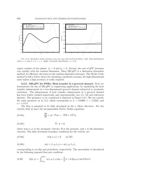
Fig. 3.13. Evolution of the variance of y1 for case (iii) of K-O problem. Left: Beta distribution
with α =1and β =4. c =1. Right: Gaussian distribution. c =0.3.
region consists of two planes: ξ1 = 0 and ξ2 = 0. Second, the cost of gPC increases
very quickly with the random dimension. Since ME-gPC is a dimension dependent
method, its efficiency decreases as the random dimension increases. The Monte Carlo
method is still a better choice for obtaining a moderate accuracy for high-dimensional
cases unless a high accuracy is really required.
3.2.3. ME-gPC for PDEs: Heat transfer in a grooved channel. Next, we
demonstrate the use of ME-gPC to engineering applications, by simulating the heat
transfer enhancement in a two-dimensional grooved channel subjected to stochastic
excitation. The phenomenon of heat transfer enhancement in a grooved channel
has been widely studied numerically and experimentally (see [11, 16] and references
therein). The geometry to be considered is depicted in Figure 3.14. We use exactly
the same geometry as in [11], which corresponds to L =6.6666, l =2.2222, and
a =1.1111.
The flow is assumed to be fully developed in the x (flow) direction. For the
velocity field we have the incompressible Navier–Stokes equations
(3.18a)
(3.18b)
∂v
∂t +(v ·∇)v = −∇Π+ν∇2 v,
∇·v =0,
where v(x,t; ω) is the stochastic velocity, Π is the pressure, and ν is the kinematic
viscosity. The fully developed boundary conditions for the velocity are
(3.19a)
(3.19b)
v(x,t; ω) =0 on∂D,
v(x + L, y, t; ω) =v(x, y, t; ω),
corresponding to no-slip and periodicity, respectively. The uncertainty is introduced
by the following imposed flow-rate condition:
(3.20)
Q(t; ω) =
� ∂DT
∂DB
u(x, y, t; ω)dy = 4
3 (1+0.2ξH(ω) sin 2πΩF t),