Discontinuous Galerkin methods Lecture 1 - Brown University

RMMC 2008
Discontinuous Galerkin methods
Lecture 1
Jan S Hesthaven
Brown University
-0.75
Jan.Hesthaven@Brown.edu x
y
y
1
0.75
0.5
0.25
0
-0.25
-0.5
-1
-1 -0.5 0 0.5 1
1
0.75
0.5
0.25
0
-0.25
-0.5
-0.75
1.203
1.142
1.081
1.019
0.958
0.896
0.835
0.774
0.712
0.651
0.590
0.528
0.467
0.405
0.344
0.283
0.221
0.160
0.099
0.037
y
1
0.75
0.5
0.25
0
-0.25
-0.5
-0.75
8.4 Scattering about a vertical cylinder in a finite-width channel -0.0881 147
10
0.75
9
test the consistency of the imposed bound-
8
7
ary conditions and investigate 0.5
6how
the geo-
0
cal model based on the linear Padé (2,2) ro-
0.02
tational velocity version we set up a test-0.25 for
0.01
open-channel flow. We seek to model the scat-
0
-0.5
tering of an incident wave field which is prop-
-0.01
y
-0.02
der positioned -0.03 in the middle of a finite-width
-0.03 -0.02 -0.01 0 0.01 0.02 0.03
x
-1
-1 -0.5 0 0.5 1
x
y
-1
-1 -0.5 0 0.5 1
x
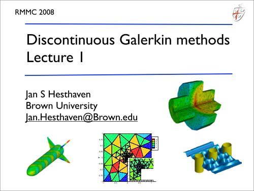
8.4 Scattering about a vertical cylinder in a finitewidth
channel
A numerical study is carried out to both
metric representation of the the domain may 0.25
affect the computed solution. In a numeri-
agating toward a bottom-mounted rigid cylin-
channel.
1
-0.75
Due to the symmetry, the solution is mathe-
y
0.02
0.01
0
-0.01
-0.02
-0.03
-0.0028
-0.0072
-0.0117
-0.0162
-0.0207
-0.0252
-0.0297
-0.0342
-0.0387
-0.0432
-0.0477
-0.0522
-0.0567
-0.0612
-0.0657
-0.0702
-0.0747
-0.0791
-0.0836
1.95E-06
1.70E-06
1.45E-06
1.20E-06
9.45E-07
6.94E-07
4.43E-07
1.92E-07
-5.90E-08
-3.10E-07
-5.61E-07
-8.12E-07
-1.06E-06
-1.31E-06
-1.57E-06
-0.03 -0.02 -0.01 0 0.01 0.02 0.03
-1
x
-1 -0.5 0 0.5 1
Figure 8.12: Scattering x of waves about a
Darmstadt International Workshop, October 2004 – p.79
cylinder in a finite-width channel.

Start by saying thanks!
• To the main organizers
• D. Stanescu and A. Porter (UWY)
• Funding agencies to enable the work
• NSF, ARO, DARPA, AFOSR, Sloan Foundation
• Collaborators over time
• Tim Warburton
• David Gottlieb
• -- and many others

A brief overview of what’s to come
• Lecture 1: Introduction, Motivation, History
• Lecture 2: Basic elements of DG-FEM
• Lecture 3: Linear systems and some theory
• Lecture 4: A bit more theory and discrete stability
• Lecture 5: Attention to implementations
• Lecture 6: Nonlinear problems and properties
• Lecture 7: Problems with discontinuities and shocks
• Lecture 8: Higher order/Global problems

springer.com
... and it goes on
• Two afternoons with hands-on exercises
• Next week: T Warburton on
2D/3D, parallel, GPU etc
Lectures and exercises
are based on text
54
Nodal Discontinuous Galerkin
Methods: Algorithms, Analysis, and
Applications
Jan S. Hesthaven • Tim Warburton
TEXTS IN APPLIED MATHEMATICS
This book discusses the discontinuous Galerkin family of computational methods
for solving partial differential equations. While these methods have been known
since the early 1970s, they have experienced a phenomenal growth in interest during
the last ten to fifteen years, leading both to substantial theoretical developments
and the application of these methods to a broad range of problems.
These methods are distinct in nature from standard methods such as finite element
or finite difference methods, often presenting a challenge in the transition
from theoretical developments to actual implementations and applications.
This book is suitable for graduate level classes in applied and computational
mathematics. The combination of an in-depth discussion of the fundamental
properties of the discontinuous Galerkin computational methods with the availability
of extensive accompanying Matlab based implementations allows students
to gain first-hand experience from the beginning without eliminating theoretical
insight.
Jan S. Hesthaven is a professor of Applied Mathematics at Brown University.
Tim Warburton is an assistant professor of Applied and Computational
Mathematics at Rice University.
isbn 978-0-387-72065-4
Hesthaven
Warburton
TAM
54
Nodal Discontinuous Galerkin Methods
54
Jan S. Hesthaven
Tim Warburton
TEXTS IN APPLIED MATHEMATICS
Nodal Discontinuous
Galerkin Methods
Algorithms, Analysis, and
Applications
www.nudg.org

Lecture 1
• Why do we need something else ?
• The new challenges
• Why high-order schemes seem a good
idea
• The good, the bad, and the ugly on ‘classic’
methods
• What we need and how we get it
• The first DG-FEM schemes we see
• A bit of history

1 PFlop/s
1 TFlop/s
Moore’s law and the performance gap
1 GFlop/s
1 MFlop/s
1 KFlop/s
Moore’s Moore s Law
Scalar
IBM 7090
UNIVAC 1
EDSAC 1
Super Scalar
CDC 7600
CDC 6600
Vector
IBM 360/195
Cray 1
Super Scalar/Vector/Parallel
TMC CM-5 Cray T3D
Cray 2
Cray X-MP
Parallel
TMC CM-2
ASCI Red
Earth
Simulator
ASCI White
Pacific
1941 1 (Floating Point operations / second, Flop/s)
1945 100
1949 1,000 (1 KiloFlop/s, KFlop/s)
1951 10,000
1961 100,000
1964 1,000,000 (1 MegaFlop/s, MFlop/s)
1968 10,000,000
1975 100,000,000
1987 1,000,000,000 (1 GigaFlop/s, GFlop/s)
1992 10,000,000,000
1993 100,000,000,000
1997 1,000,000,000,000 (1 TeraFlop/s, TFlop/s)
2000 10,000,000,000,000
2003 35,000,000,000,000 (35 TFlop/s)
1950 1960 1970 1980 1990 2000 2010
Current predictions in required
performance needs show a large
H. Meuer, H. Simon, E. Strohmaier, & JD
and growing gap, known as the
- Listing of the 500 most powerful
Computers in the World
- Yardstick: Rmax from LINPACK MPP
performance gap
Ax=b, dense problem
ate
TPP performance
!"#$%&'#$()&#*)#+$,-./01&*2$,"344#*2#
3
Raw performance largely
driven by innovation in
hardware has so far followed
Moore’s law: ‘Bang-per-buck’
doubles every 24 months
38+

What is causing this growing gap ?
Our way of doing science is being transformed as
simulation science matures, enabling entirely new
ways of addressing problems of national interest.
Solving ‘real’ problems introduce new challenges:
• Modeling of very large scale complex systems, incl
unsteady, multi-physics, multi-scale problems
• Treatment of uncertainties and stochastic effects
• Interaction/assimilation with experimental data
• Very large scale data manipulation and
visualization ‘from data to knowledge’
• Very large scale optimization, estimation, design

Can we close the gap ?
FIGURE 1 (software infrastructure)
.. and by paying careful
attention to the dirty
Which algorithms are needed for the next generation of scientific problems? They should
address the statistical challenges of massive dimensions, and the heterogeneous multiscale nature
of the science driver problems.
Infrastructure Issues
Databases of software should be made available to practitioners. Automatic assistance needs to
be provided to help locate the most appropriate algorithm for a given problem and data.
Problems such as how do you communicate the meta-assumptions of your data need to be
resolved. details
We need to be able to assure quality whenever possible, but not set standards
prematurely or too strictly as to inhibit development of new tools and technologies.
‘Parallel scaling is not all’
RECOMMENDATIONS
Software Infrastructure Support
To develop, manage, leverage and maintain the software infrastructure needed for the next
generation of science, sustained infrastructure and facility support will be required.
.. only by developing more
advanced algorithms

Can we close the gap ?
It is the algorithms, their analysis, and implementation
that are the hard components of this quest toward
real simulations
• Complex to develop and implement
• Very labor intensive (manpower, hero program.)
• Long lived (20-30 years vs 3-5 for hardware)
• Costly !
Question:
Can we hope to mimic the success of standard packages
for linear algebra and ODE’s on PDE’s ?

What should we require ?
The challenges are very substantial
• Steady and unsteady
• Complex geometries
• Multi physics
• Many scales in space and time
We must require a number of key properties
• Flexibility in both geometry and problem types
• Robustness
• Efficiency/high performance/hardware suitable
• ... high-order/variable order accuracy
This is a tall order at best !

Why high-order accuracy ?
We may be able to agree on most of the properties -
except perhaps that on high-order
General concerns/criticism
• High-order accuracy is not needed for real appl.
• The methods are not robust
• They only work for smooth problems
• They are hard to do in complex geometries
• They are too expensive
• etc
After having worked on these methods
for 15 years, I have heard them all

n June 7, 2006 9:29
Why high-order accuracy ?
Let us first define a high-order method as one having
a truncation order exceeding 2
From local to global approximation
Let us consider a simple time-dependent problem
ample 1.1 Consider the wave equation
∂u
∂t
= −2π ∂u
∂x
u(x, 0) = e sin(x) ,
0 ≤ x ≤ 2π, (1.1)
h periodic boundary conditions.
The We exactshall solution solve to Equation it using (1.1) two isdifferent a right-moving ways wave of the form
u(x, t) = e sin(x−2πt) • A standard 2nd order finite difference method
,
• A Fourier spectral method - an ‘infinite order’ method
, the initial condition is propagating with a speed 2π.

U(x,
1.5
Why high-order accuracy ?
0.5
U(x,t)
U(x,t)
1.0
0.0
0 p/2 p
x
3p/2 2p
3.0
2.5
2.0
1.5
1.0
0.5
N = 200
t = 100.0
0.0
0 p/2 p
x
3p/2 2p
3.0
2.5
2.0
1.5
1.0
0.5
N = 200
t = 200.0
0.0
0 p/2 p
x
3p/2 2p
Finite diff.
N=200
U(x,
U(x,t)
U(x,t)
1.5
1.0
0.5
0.0
0 p/2 p
x
3p/2 2p
3.0
2.5
2.0
1.5
1.0
0.5
N = 10
t = 100.0
0.0
0 p/2 p
x
3p/2 2p
3.0
2.5
2.0
1.5
1.0
0.5
N = 10
t = 200.0
0.0
0 p/2 p
x
3p/2 2p
Fourier
N=10
Figure 1.2 An illustration of the impact of using a global method for problems
requiring long time integration. On the left we show the solution of Equation (1.1)
as computed using a second-order centered-difference scheme. On the right we
show the same problem solved using a global method. The full line represents the
computed solution, while the dashed line represents the exact solution.
T=100
T=200
The Fourier
method is about
10 times faster !

Why high-order accuracy ?
Too simple you may say
a)
U(x)
5
4
3
2
1
0
-1
-2
-3
-4
-5
0 ! 2!
x
N=64
t=0.0
b)
U(x)
5
4
3
2
1
0
-1
-2
-3
-4
-5
0 ! 2!
x
N=64
t=100.0
Lack of smoothness does not
destroy the superior properties
... but is high-order accuracy really needed
and what is the cost -- can’t we just run the 2nd
order scheme with more points ?

We arrive at a more straightforward measure o
Why high-order accuracy ?
introducing ...high-order pm(εp, cont’ ν) as a measure of the numbe
ds ν i.e., the error grows linearly in time.
e straightforward measure of the error of the scheme b
) as a measure of the number of points per waveleng
required to guarantee a phase error, ep ≤ εp, afte
How do I solve the problem to a given accuracy, ,
for a specific period of time, , most efficiently ?
Solving wave problems in d-dimensions to time t with
a phase error, ep ≤ εp, after ν periods for a 2m-ord
scheme. accuracyIndeed, from Equation (1.13) we directly
εp this translates into
νπ
rder cont’
Equation (1.13) we directly obtain the lower bounds
νπ
p1(ε, ν) ≥ 2π , (1.14
3εp
p2(ε, ν) ≥ 2π 4
p1(ε, ν) ≥ 2π ,
3εp
πν p2(ε, ν) ≥ 2π
,
15εp
4
d
2m ν
Memory ∝ , Work ∝ (2m)
εp
πν
15εp
d d+1
2m ν
ν .
εp
Here So 2m we >2also advantageous have in cases where
• 2m = order of the scheme
εp ≪ 1, i.e., when high accuracy is required.
actical way to address this is by using a
r-order scheme – Truncation error exceeds 2.
• d = dimension of the problem
hows that the phase error behaves as
• the number of points per wavelength
cific error εp.
em(p, ν) ∝ νp −2m ⇒ p(ν, εp) ∝ 2m
ν
,
ν ≫ 1, i.e., when long time integration is needed.
on pm, ensuring a specific error εp.
d>1, i.e., for multi-dimensional problems.
It is immediately apparent that for long time inte
pparent that for long time integrations (large ν), p2 ≪ p
pm < 10, i.e., efficient discretizations of large problems.
justifying the use of high-order schemes. In the f
high-order schemes. In the following examples, we wi
εp

Why
14
high-order
From local
accuracy
to global approximation
?
350
300
250
200
150
100
50
e p = 0.1
0
0 0.25 0.5 0.75 1
n
W 1
W 2
W 3
3500
3000
2500
2000
1500
1000
500
0
e p = 0.01
W 1
W 2
W 3
0 0.25 0.5 0.75 1
n
High-order Figure 1.3 is The the growthright of the work solution function, Wm, forif various : finite difference
schemes is given as a function of time, ν, in terms of periods. On the left we show
the growth for a required phase error of εp = 0.1, while the right shows the result
• High accuracy is required - and it increasingly is !
of a similar computation with εp = 0.01, i.e., a maximum phase error of less than
1%. • Long time integration is needed
• High-dimensional problems (3D) are considered
• Memory restrictions become a bottleneck
• .. apart from that, these methods are superior
for hardware with deep memory hierarchies
where C F Lm = c t
refers to the C F L bound for stability. We assume that the
x
fourth-order Runge–Kutta method will be used for time discretization. For this
method it can be shown that C F L1 = 2.8, C F L2 = 2.1, and C F L3 = 1.75.
Thus, the estimated work for second, fourth, and sixth-order schemes is
W1 30ν ν
ν
, W2 35ν , W3 48ν 3
ν
. (1.15)
εp
εp
εp

to advance the equations in time, there is likewise a wide v
forHow the integration do we achieve of systems this of? ordinary differential equ
choose among. With such a variety of successful and well te
is tempted Let us consider to ask why a few there well known is a need schemes to consider and their yet anoth
basic To appreciate properties this, to understand let us beginwhat by attempting is needed. to unders
and weaknesses of the standard techniques. We consider th
scalar Consider conservation the basic lawequation for the solution u(x, t)
∂u
∂t
+ ∂f
∂x
= g, x ∈ Ω,
subject All schemes to an appropriate involve two set choices of initial conditions and boun
the boundary, ∂Ω. Here f(u) is the flux, and g(x, t) is some
function. • In which way does one approximate the solution ?
• The In which construction way should of any the numerical approximation method satisfy for solving a
equation the requires PDE ? one to consider the two choices:
• How does one represent the solution u(x, t) by an app

Finite difference methods
roduction
neighborhood of each grid point xk 1 Introduction
, the solution and the flux are as
d by local polynomials
• The local approximation is a 1D polynomial
• The equation is satisfied in a pointwise manner
t, in the neighborhood of each grid point xk , the solution and the flux are assumed to be w
roximated by local polynomials
1 Introduction
own in space and spatial derivatives are approximated by difference metho
at is, the conservation law is approximated as
duh(xk ,t)
+
dt
fh(xk+1 ,t) − fh(xk−1 ,t)
hk + hk−1 = g(x k ∈ [x
,t), (1
k−1 ,x k+1 2
]: uh(x, t) = ai(t)(x − x
i=0
k ) i 2
, fh(x, t) = bi(t)(x −
i=0
efficients ai(t) and bi(t) are found by requiring that the approximat
he grid points, xk x ∈ [x
. Inserting these local approximations into Eq.(1.1
k−1 ,x k+1 2
]: uh(x, t) = ai(t)(x − x
i=0
k ) i 2
, fh(x, t) = bi(t)(x − x
i=0
k ) i ,
re the coefficients ai(t) and bi(t) are found by requiring that the approximate function in
ates at the grid points, xk . Inserting these local approximations into Eq.(1.1), results in
dual
x ∈ [x k−1 ,x k+1 ]: Rh(x, t) = ∂uh + ∂fh − g(x, t).

Finite difference schemes
• Main benefits
• Simple to implement and fast
• High-order is feasible
• Explicit in time
• Direction can be exploited - upwind
• Strong theory
• Main problem
• Simple local approximation and geometric
flexibility are not agreeable

to unstructured grids in high dimensions, thus ensuring the desired g
more, the construction of the interface fluxes can be done in various
needs to abandon the simple one-dimensional approximation in favor of som
thing more general. The most natural approach is to introduce an elemen
tforward.
Finite volume methods
based discretization. Hence, we assume that Ω is represented by a collecti
of elements, D k lem and the subsequent evaluation of the fluxe
s
to
reconstruction
the particular equations
problem
(see, e.g.,
and
[218,
the
303]).
subsequent
This is particularly
evalu
nt nonlinear waysconservation and, typically the laws. details simplexes of or cubes, thisorganized lead toin different
an unstructur
ressed in many different ways and the details of this
If, however, we wish to increase the order of accuracy of the met
emerges. Consider again the problem in one dimension. We wish to rec
the interface and we seek a local polynomial, uh(x) of the form
manner to fill the physical domain.
A method closely related to the finite difference method, but with add
geometric flexibility, is the finite volume method. In its simplest form, t
solution u(x, t) is approximated on the element by a constant, uk (t), at t
center, xk , of the element. Thisx is ∈ introduced [x into Eq. (1.1) to recover t
cellwise residual
k−1/2 ,x k+3/2 , f ]: uh(x) =a + bx.
k+1/2 = f(u k+1/2 u ),
k+1/2 = uk+1 + uk n to the reconstruction problem is to use
le and natural solution to the reconstruction proble
k+1/2 = u k+1 + u k
We then require
2
• The local approximation is a cell average
x ∈ D k : Rh(x, t) = ∂uk
∂t + ∂f(uk )
k+1/2
x ∂x
uh(x) dx = h k u k ,
− g(x, t),
x k+3/2
rnatively, one could be tempted to simply take
where the element is defined as D k =[xk−1/2 ,xk+1/2 ] with xk+1/2 = 1
2 (xk
xk+1 x
). In the finite volume method we require that the cell average of t
residual vanishes identically, leading to the scheme
k−1/2
xk+1/2 • The equation is satisfied on conservation form
uh(x) dx = h k
k duk
h
dt + f k+1/2 − f k−1/2 = h k g k to recover the two coefficients. The reconstructed value of the solu
f(uh(x
, (1.
k+1/2 ,
)) can then be evaluated.
2
2
To reconstruct the interface values at a higher accuracy we can c
local h this solution turns of the out form to not be a good idea for general
f k+1/2 = f(uk )+f(u k+1 )
t be a good idea for general nonlinear problem
for each cell. Note that the approximation and the scheme is purely loc
uidistant grids these methods all reduce to the finite
p
2
, f k+1/2 =
ewise for f k−1/2 . Alternatively, one could be tempte
f k+1/2 = f(uk )+f(u k

evaluation of these fluxes is not straightforward.
Finite
This reconstruction
volume
problem
methods
and the subsequent evaluation of the fluxes at
the interfaces can be addressed in many different ways and the details of this
lead to different finite volume methods. A simple solution to the reconstruction
problem is to use
The key challenge is one of reconstruction
u k+1/2 = uk+1 + uk , f
2
k+1/2 = f(u k+1/2 ),
• Main benefit
• Robust and fast due to locality
• Complex geometries 2
• Well suited for conservation laws
• Explicit in time
and likewise for f k−1/2 . Alternatively, one could be tempted to simply take
f k+1/2 = f(uk )+f(uk+1 )
,
although this turns out to not be a good idea for general nonlinear problems.
For linear problems and equidistant grids these methods all reduce to the finite
difference method. However, one easily realizes that the formulation is less
restrictive in terms of the grid structure; that is, the reconstruction of solution
values at the interfaces is a local procedure and generalizes straightforwardly
to unstructured grids in high dimensions, thus ensuring the desired geometric
• Main problem
• Inability to achieve high-order on general grids
due to extended stencils
• Grid smoothness requirements

where the piecewise linear shape function, N
Finite element methods
We begin by splitting the solution into elements as
i (xj )=δij is the basis function
and uk = u(xk ) remain as the unknowns.
To recover the scheme to solve Eq. (1.1), we define a space of test functions,
x ∈ D
Vh, and require that the residual is orthogonal to all test functions in this
space as
∂uh ∂fh
+ − gh φh(x) dx =0, ∀φh ∈ Vh.
Ω ∂t ∂x
The details of the scheme is determined by how this space of test functions is
defined. A classic choice, leading to a Galerkin scheme, is to require the that
spaces spanned by the basis functions and test functions are the same. In this
particular case we thus assume that
k : uh(x) =u(x k x − xk+1
)
xk − xk+1 + u(xk+1 )
x
where the linear Lagrange polynomial, ℓk i (x), i
ℓ k x − xk+1−
i (x) =
xk+i − xk+ With this local element-based model, each elem
other element (e.g., D k−1 and D k share xk ). W
of uh as
• The solution is defined in a nonlocal manner
φh(x) =
K
v(x k )N k (x).
uh(x) =
k=1
• The equation is satisfied globally
K
u(x k )N k (x) =
Since the residual has to vanish for all φh ∈ Vh, this amounts to
∂uh ∂fh
+ − gh N
Ω ∂t ∂x j where the piecewise linear shape function, N
(x) dx =0,
for j =1...K. Straightforward manipulations yield the scheme
i (
and uk = u(xk ) remain as the unknowns.
To recover the scheme to solve Eq. (1.1), we
Vh, and require that the residual is orthogon
k=1
k

has to vanish for all φh ∈ Vh, this amounts to
Finite element methods
∂uh ∂fh
+ − gh N
∂t ∂x j
∂uh ∂fh
+
(x) Ωdx
=0, ∂t ∂x
Ω
This yields the global equation
aightforward manipulations yield the scheme
− gh
N j (x) dx =0,
for j =1. . . K. Straightforward manipulations yield the scheme
where
M duh
dt + Sf h = Mgh, M duh
dt + Sf h = Mgh, (1.4)
Mij =
Ω
N i (x)N j (x) dx, Sij =
• Main benefits
• High-order accuracy and complex geometries
can be combined
Ω
N i j dN
(x)
dx dx,
reflects the globally defined mass matrix and stiffness matrix, respectively. We
vectors of unknowns, uh = [u1 , . . . , uNp T ] , of fluxes, f h = [f1 , . . . , f Np T ] , and
gh =[g1 , . . . , gNp T ] , given on the Np nodes.
This approach, which reflects the essence of the classic finite element method [182,
clearly allows different element sizes. Furthermore, we recall that a main motivation f
methods beyond the finite volume approach was the interest in higher-order approxi
extensions • Main are problems relatively simple in the finite element setting and can be achieved by add
degrees of freedom to the element while maintaining shared nodes along the faces o
[197]. • Implicit In particular, in one time can have different orders of approximation in each element, the
local • Not changes well in both suited size and for order, problems known as hp-adaptivity with direction (see, e.g., [93, 94]).
However, the above discussion also highlights disadvantages of the classic continu
ment formulation. First, we see that the globally defined basis functions and the req

volume methods (FVM), and finite element methods (FEM), as compared with the
discontinuous Galerkin finite element method (DG-FEM)]. A represents success,
Lets summarize the observations
while ✕ indicates a short-coming in the method. Finally, a () reflects that the
method, with modifications, is capable of solving such problems but remains a less
natural choice.
Complex High-order accuracy Explicit semi- Conservation Elliptic
geometries and hp-adaptivity discrete form laws problems
FDM ✕
FVM ✕ ()
FEM ✕ ()
DG-FEM ()
residual destroys the locality of the scheme and introduces potential problems
with the stability for wave-dominated problems. On the other hand, this is
precisely the regime where the finite volume method has several attractive
features.
An intelligent combination of the finite element and the finite volume
methods, utilizing a space of basis and test functions that mimics the finite
element method but satisfying the equation in a sense closer to the finite
volume method, appears to offer many of the desired properties. This combination
is exactly what leads to the discontinuous Galerkin finite element
method (DG-FEM).
To achieve this, we maintain the definition of elements as in the finite
element scheme such that D k =[xk ,xk+1 What we need is a scheme that combines
• The local high-order/flexible element of FEM
• The local statement on the equation for FVM
These are exactly the components of the
Discontinuous Galerkin Finite Element Method
]. However, to ensure the locality

D
So lets see how we can achieve this
k = D k
uv dx, u k
D =(u, u) k
D ,
oken inner product and norm
h =
K
(u, v) k
D , u
k=1
2 Ω,h =(u, u) Ω,h .
t Ω is only approximated by the union of D k , that is
K
Ω Ωh = D
k=1
k 2.2 Basic elements of the sch
D
,
stinguish the two domains unless needed.
cal information as well as information from the neighintersection
between two elements. Often we will refer
tersections in an element as the trace of the element.
cuss here, we will have two or more solutions or boundme
physical location along the trace of the element.
k Dk+1 Dk-1 x 1
l =L xk-1 xK r =xl k xk r =xl k+1
r =R
Fig. 2.1. Sketch of the geometry for simple one-dimensional ex
basis, ψn(x). A simple example of this could be ψn(x) =xn−1 .
local grid points, xk i ∈ Dk Consider the linear scalar wave equation
∂u ∂f(u)
+ =0, x ∈ [L, R] =Ω,
∂t ∂x
where the linear flux is given as f(u) =au. This is subject to the appro
initial conditions
u(x, 0) = u0(x).
Boundary conditions are given when the boundary is an inflow bou
that is
u(L, t) =g(t) if a ≥ 0,
u(R, t) =g(t) if a ≤ 0.
We approximate Ω by K nonoverlapping elements, x ∈ [x
, and express the polynomial through th
k l ,xkr] = D
illustrated in Fig. 2.1. On each of these elements we express the local so
as a polynomial of order N = Np − 1
x ∈ D k : u k Np
h(x, t) = û k Np
n(t)ψn(x) = u k h(x k i ,t)ℓ k l r
xpress the local solution as a polynomial of order N
Np
k k
: uh(x, t) = û
n=1
It is the multi-element component of FEM/FVM which
gives the geometric flexibility
i (x).
k Np
n(t)ψn(x) = u
i=1
k h(x k i ,t)ℓ k i (x).
two complementary expressions for the local solution. In the first one,
we use a local polynomial basis, ψn(x). A simple example of this could
lternative form, known as the nodal representation, we introduce Np =
∈ D k , and express the polynomial through the associated interpolating
). The connection between these two forms is through the definition of
ûk n. We return to a discussion of these choices in much more detail later;
e that we have chosen one of these representations.
, t) is then assumed to be approximated by the piecewise N-th order
uh(x, t),
K
u(x, t) uh(x, t) = u
k=1
k and the solution is represented as
h(x, t),
native form, known as the nodal representation, we introduce N
(x). The connection betwe
forms is through the definition of the expansion coefficients, ûk i=1
n. W
Here, we have introduced two complementary expressions for the loca
a
tion.
discussion
In the first
of these
one, known
choices
as
in
the
much
modal
more
form,
detail
we use
later;
a local
for now
polyn
assume that we have chosen one of these representations.
The global solution u(x, t) is then assumed to be approxim
piecewise N-th order polynomial approximation uh(x, t),
interpolating Lagrange polynomial, ℓk n=1 i
with a high-order local basis as in FEM:
• on modal form
• on nodal form

sic understanding of the schemes through a simple example.
The first DG schemes
first schemes
So let us consider the scalar problem
e linear scalar wave equation
∂u ∂f(u)
+ =0, x ∈ [L, R] =Ω,
∂t ∂x
near flux is given as f(u) =au. This is subject to the appropriate initial condit
u(x, 0) = u0(x).
onditions are given when the boundary is an inflow boundary, that is
u(L, t) =g(t) if a ≥ 0,
u(R, t) =g(t) if a ≤ 0.
ate Ω by K nonoverlapping elements, x ∈ [x k l ,xk r]=D k , as illustrated in Fig.
e elements we express the local solution as a polynomial of order N
x ∈ D k : u k h(x, t) =
Np
n=1
û k n(t)ψn(x) =
Np
i=1
u k h(x k i ,t)ℓ k i (x).

sic understanding of the schemes through a simple example.
The first DG schemes
firstx schemes ∈ D k : u k k x − xk+1
h(x) =u
xk x − xk
+ uk+1
− xk+1 xk+1 1
= u
− xk k+i ℓ k i (x) ∈ Vh,
So let us consider the scalar problem
e linear scalar wave equation
ise for the flux, f
∂u ∂f(u)
+ =0, x ∈ [L, R] =Ω,
∂t ∂x
near flux is given as f(u) =au. This is subject to the appropriate initial condit
We form the local residual
u(x, 0) = u0(x).
onditions are given when the boundary is an inflow boundary, that is
k h . The space of basis functions is defined as Vh = ⊕K
k
k=1 ℓi of piecewise polynomial functions. Note in particular that there is no restric
ss of the test functions between elements.
the finite element case, we now assume that the local solution can be well re
pproximation uh ∈ Vh and form the local residual
x ∈ D k : Rh(x, t) = ∂uk h
∂t + ∂f k h − g(x, t),
∂x
u(L, t) =g(t) if a ≥ 0,
u(R, t) =g(t) if a ≤ 0.
ate Ω by K nonoverlapping elements, x ∈ [xk l ,xkr]=D k lement. Going back to the finite element scheme, we recall that the global c
ual are the source of the global nature of the operators M and S in Eq. (1.4).
equire that the residual is orthogonal to all test functions φh ∈ Vh, leading t
, as illustrated in Fig.
e elements we express the local solution as a polynomial of order N
x ∈ D k : u k h(x, t) =
Np
n=1
û k n(t)ψn(x) =
Np
i=1
i=0
u k h(x k i ,t)ℓ k i (x).

sic understanding of the schemes through a simple example.
The first DG schemes
firstx schemes ∈ D k : u k k x − xk+1
h(x) =u
xk x − xk
+ uk+1
− xk+1 xk+1 1
= u
− xk k+i ℓ k i (x) ∈ Vh,
So let us consider the scalar problem
e linear scalar wave equation
ise for the flux, f
∂u ∂f(u)
+ =0, x ∈ [L, R] =Ω,
∂t ∂x
near flux is given as f(u) =au. This is subject to the appropriate initial condit
We form the local residual
u(x, 0) = u0(x).
onditions are given when the boundary is an inflow boundary, that is
k h . The space of basis functions is defined as Vh = ⊕K
k
k=1 ℓi of piecewise polynomial functions. Note in particular that there is no restric
ss of the test functions between elements.
the finite element case, we now assume that the local solution can be well re
pproximation uh ∈ Vh and form the local residual
x ∈ D k : Rh(x, t) = ∂uk h
∂t + ∂f k h − g(x, t),
∂x
u(L, t) =g(t) if a ≥ 0,
u(R, t) =g(t) if a ≤ 0.
ate Ω by K nonoverlapping elements, x ∈ [xk l ,xkr]=D k lement. Going back to the finite element scheme, we recall that the global c
and require this to vanish locally in a Galerkin sense
ual are the source of the global nature of the operators M and S in Eq. (1.4).
equire that the residual is orthogonal to all test functions φh ∈ Vh, leading t
D , as illustrated in Fig.
e elements we express the local solution as a polynomial of order N
k
Rh(x, t)ℓ k j (x) dx =0,
x ∈ D k : u k Np
h(x, t) = û k Np
n(t)ψn(x) = u k h(x k i ,t)ℓ k and the fact that we have duplicated solutions at all interface nodes.
is locality also appears problematic as this statement does not
i (x). allow one to recov
obal solution. Furthermore, the points at the ends of the elements are shared by
n=1
i=1
i=0
1 Introduction
The problem is that all elements are now disconnected
due to the local statement on the residual!
t functions, ℓ k j (x). The strictly local statement is a direct consequence of Vh bein

allow one to recover a meaningful global solution. Furthermore, the points at
theThe ends of first the elements DG schemes
are shared by two elements so how does one ensure
uniqueness of the solution at these points?
These problems are overcome by observing that the above local statement
is very Let similar us apply to that Gauss’s recovered theorem in the finite volume method. Following this
line of thinking, let us use Gauss’ theorem to obtain the local statement
D k
∂uk h
∂t ℓkj − f k dℓ
h
k j
dx − gℓkj dx = − f k h ℓ kx j
k+1
xk .
What remains now is to understand what the right-hand side means. This is,
however, easily understood by considering the simplest case where ℓk j (x) is
a constant, in which case we recover the finite volume scheme in Eq. (1.3).
Hence, the main purpose of the right-hand side is to connect the elements.
This is further made clear by observing that both element D k and element
D k+1 depends on the flux evaluation at the point, xk+1 , shared among the two
elements. This situation is identical to the reconstruction problem discussed
previously for the finite volume method where the interface flux is recovered
by combining the information of the two cell averages appropriately.
At this point it suffices to introduce the numerical flux, f ∗ k-1
k+1
k
, as the unique
value to be used at the interface and obtained by combining information from
both We elements. have multiple With this we solutions recover the and scheme we need to pick one !

D
The first DG schemes
k+1 depends on the flux evaluation at the point, xk+1 , shared among the t
elements. This situation is identical to the reconstruction problem discus
previously for the finite volume method where the interface flux is recove
by combining the information of the two cell averages appropriately.
At this point it suffices to introduce the numerical flux, f ∗ , as the uni
value to be used at the interface and obtained by combining information fr
both elements. With this we recover the scheme
D k
∂uk h
∂t ℓkj − f k dℓ
h
k j
dx − gℓkj dx = − f ∗ ℓ kx j
k+1
xk ,
or, by applying Gauss’ theorem once again,
Rh(x, t)ℓ k j (x) dx = (f k h − f ∗ )ℓ kx j
k+1
2.3 Toward more general formulations 27
ux , f
.
∗ = f ∗ (u −
h ,u+ h ), is again at the very heart of the formulation.
hat it is consistent [i.e., single valued as f(uh) =f ∗ (uh,uh)] when
originating in the hugely successful development of monotone finite
0s, is to require that the flux be chosen so that the scheme reduces
order/finite volume limit. This is ensured by requiring that f ∗ remains now is to understand what the right-hand side means. This is, however, ea
ood by considering the simplest case where ℓ
The lack of solution uniqueness at the interface is
addressed as in FVM by a numerical flux
(a, b)
ment and nonincreasing in the second argument [218].
tonewith flux the is thecorresponding E-flux [251], satisfying strong form being
k j (x) is a constant, in which case we recover
olume scheme in Eq.(1.3). Hence, the main purpose of the right-hand side is to connect
ts. This is further made clear by observing that both element D k and element D k+1 depe
flux evaluation at the point, xk+1 , shared among the two elements. This situation is ident
econstruction problem discussed previously for the finite volume method where the inter
recovered by combining the information of the two cell averages appropriately.
this point it suffices to introduce the numerical flux, f ∗ , as the unique value to be used
erface and obtained by coming information from both elements. With this we recover
D k
∂uk h
∂t ℓkj − f k dℓ
h
k j
dx − gℓkj dx = − f ∗ ℓ kx j
k+1
xk ,
pplying Gauss’ theorem once again,
D k ∂t ℓ j − f h dx − gℓ j dx = − f h ℓ j x k .
D k
These two formulations are the discontinuous Galerkin finite element (D
FEM) schemes for the scalar conservation law in weak and strong form,
spectively. Note that the choice of the numerical flux, f ∗ ∈ [a, b] : (f
, is a central elem
∗ (a, b) − f(v))(b − a) ≤ 0,
D
l and external value, respectively. The classic finite volume literarical
fluxes with the above properties and we will not attempt to
k
Rh(x, t)ℓ k j (x) dx = (f k h − f ∗ )ℓ kx j
k+1
xk .
two formulations are the discontinuous Galerkin finite element (DG-FEM) schemes for
Naturally, the choice of the flux is important !
onservation law in weak and strong form, respectively. Note that the choice of the numer
, is a central element of the scheme and is also where one can introduce the dynamics of
ll [e.g., primarily by upwinding consider through the Lax-Friedrichs the flux as in a finite flux along volumethe method(FVM)]. normal, ˆn,
x k

1 Introduction
The basics of DG-FEM
we have the vectors of local unknowns, u k , of fluxes, f k , and the forcing, g k , all given on the
in each element. Given the duplication of unknowns at the element interfaces, each vector is
ng. Furthermore, we have ℓ k (x) = [ℓk 1(x), . . . , ℓk Np (x)]T and the local matrices
To simplify the notation, introduce
M k ij =
D k
ℓ k i (x)ℓ k j (x) dx, S k ij =
1 Introduction 9
ℓ
1 Introduction 9
k i (x) dℓkj dx dx.
of the scheme and is also where one can introduce knowledge of the dynamics
of the problem [e.g., by upwinding through the flux as in a finite volume
method (FVM)].
To mimic the terminology of the finite element scheme, we write the two
local elementwise schemes as
M k duk h
dt − (Sk ) T f k h − M k g k h = −f ∗ (x k+1 )ℓ k (x k+1 )+f ∗ (x k )ℓ k (x k of the scheme and is also where one can introduce knowledge of the dynamics
of the problem [e.g., by upwinding through the flux as in a finite volume
method (FVM)].
To mimic the terminology of the finite element scheme, we write the two
local elementwise schemes as
)
M
and
k duk h
dt − (Sk ) T f k h − M k g k h = −f ∗ (x k+1 )ℓ k (x k+1 )+f ∗ (x k )ℓ k (x k to obtain the two basic forms of DG-FEM
Weak:
)
and
M k duk h
dt + Skf k h − M k g k h =(f k h (x k+1 ) − f ∗ (x k+1 ))ℓ k (x k+1 )
−(f k h (x k ) − f ∗ (x k ))ℓ k (x k M
). (1.5)
k duk h
dt + Skf k h − M k g k h =(f k h (x k+1 ) − f ∗ (x k+1 ))ℓ k (x k+1 )
−(f k h (x k ) − f ∗ (x k ))ℓ k (x k e the structure of the DG-FEM is very similar to that of the finite element method (FEM), there
veral fundamental differences. In particular, the mass matrix is local rather than global and
can be inverted at very little cost, yielding a semidiscrete scheme that is explicit. Furthermore
refully designing the numerical flux to reflect the underlying dynamics, one has more flexibility
in the classic FEM to ensure stability for wave-dominated problems. Compared with the FVM
G-FEM overcomes the key limitation on achieving high-order accuracy on general grids by
ing this through the local element-based basis. This is all achieved while maintaining benefits
as local conservation and flexibility in the choice of the numerical flux.
ll of this, however, comes at a price – most notably through an increase in the total degrees
Strong:
edom as a direct result of the decoupling of the elements. For linear elements, this yields a
ling in the total number of degrees of freedom compared to the continuous FEM as discussed
. For certain problems, this clearly becomes an issue of significant importance; that is, if we
a steady solution and need to invert the discrete operator S in Eq.(1.5) then). the associated (1.5)
utational work scales directly with the size of the matrix. Furthermore, for problems where
exibility in the flux choices and the locality of scheme is of less importance (e.g., for elliptic
ems), the DG-FEM is not as efficient as a better suited method like the FEM.
Here we have the vectors of local unknowns, uk h , of fluxes, f k h, and the forcing,
gk Here we have the vectors of local unknowns, u
h , all given on the nodes in each element. Given the duplication of
k h , of fluxes, f k h, and the forcing,
gk h , all given on the nodes in each element. Given the duplication of
D k

L 2 -errors when solving the wave equation using K elements each
on of the number of elements, K, and the order of the local approximation, N. In
Example 2.4. Consider Eq. (2.1) as
results,
A first example
as . Notewe that observe forseveral N = things. 8, the First, finite the scheme precision is clearly dominates convergentand and dest there
to a converged result; one can increase the local ∂uorder
of ∂uapproximation,
N, and/or
se the number of elements, K.
− 2π =0, x ∈ [0, 2π],
∂t ∂x
Let us consider a simple example
er Eq. (2.1) as
∂u ∂u
− 2π =0, x ∈ [0, 2π],
∂t ∂x
ary conditions and initial condition as
u(x, 0) = sin(lx), l = 2π
λ ,
ength. We use the strong form, Eq. (2.8), although for this simple example, the
ntical results. The nodes are chosen as the Legendre-Gauss-Lobatto nodes as we
il in Chapter 3. An upwind flux is used and a fourth-order explicit Runge-Kutta
to integrate the equations in time with the timestep chosen small enough to
errors can be neglected (See Chapter 3 for details on the implementation).
list a number of results, showing the global L2 with periodic boundary conditions and initial condition as
u(x, 0) = sin(lx), l =
-error at final time T = π as a
ber of elements, K, and the order of the local approximation, N. Inspecting
serve several things. First, the scheme is clearly convergent and there are two
result; one can increase the local order of approximation, N, and/or one can
of elements, K.
2π
λ ,
where λ is the wavelength. We use the strong form, Eq. (2.8), although
weak form yields identical results. The nodes are chosen as the Legendre
shall discuss in detail in Chapter 3. An upwind flux is used and a fourthmethod
is employed to integrate the equations in time with the times
ensure that timestep errors can be neglected (See Chapter 3 for details
In Table 2.1 we list a number of results, showing the global L2-err function of the number of elements, K, and the order of the local ap
these results, we observe several things. First, the scheme is clearly co
roads to a converged result; one can increase the local order of approxi
increase the number of elements, K.
Table 2.1. Global L 2 2.1. Global L
-errors when solving the wave equation using K elem
of approximation, N. Note that for N = 8, the finite precision dominate
convergence rate.
2 -errors when solving the wave equation using K elements each with a lo
roximation, N. Note that for N = 8, the finite precision dominates and destroys the
gence rate.
N\ K 2 4 8 16 32 64 Convergence rate
1 – 4.0E-01 9.1E-02 2.3E-02 5.7E-03 1.4E-03 2.0
2 2.0E-01 4.3E-02 6.3E-03 8.0E-04 1.0E-04 1.3E-05 3.0
4 3.3E-03 3.1E-04 9.9E-06 3.2E-07 1.0E-08 3.3E-10 5.0
8 2.1E-07 2.5E-09 4.8E-12 2.2E-13 5.0E-13 6.6E-13 9.0
e rate by which the results converge are not, however, the same when changing N a
fine h =2π/K as a measure of the size of the local element, we observe that
u − uhΩ,h ≤ Ch N+1 2 4 8 16 32 64 Convergence r
– 4.0E-01 9.1E-02 2.3E-02 5.7E-03 1.4E-03 2.0
2.0E-01 4.3E-02 6.3E-03 8.0E-04 1.0E-04 1.3E-05 3.0
3.3E-03 3.1E-04 9.9E-06 3.2E-07 1.0E-08 3.3E-10 5.0
2.1E-07 2.5E-09 4.8E-12 2.2E-13 5.0E-13 6.6E-13 9.0
asThe a measure error clearly of the behaves size of the as local element, we observe tha
u − uhΩ,h ≤ Ch
.
it is the order of the local approximation that gives the fast convergence rate. The c
es not depend on h, but it may depend on the final time, T , of the solution. To highli
N+1 .
r of the local approximation that gives the fast convergence ra
ich the results converge are not, however, the same when chang
on h, but it may depend on the final time, T , of the solution. T

ount of history
A brief history
alerkin finite element method (DG-FEM) appears to have been
solving the steady-state neutron transport equation
• DG-FEM was first proposed by Reed/Hill in 1973
σu + ∇ · (au) =f,
• First analysis (Lesaint, Raviart,1974) showing in
general and optimal for special
grids.
nstant, a(x) is piecewise constant, and u is the unknown. The fi
sented in [217], showing O(h
• Sharp analysis (Johnson 1986) showed
N )-convergence on a general triangu
rate, O(hN+1 ), on a Cartesian grid of cell size h and with a lo
der N. This result was later improved in [190] to O(hN+1/2 O(h
)-c
ptimality of this convergence rate was subsequently confirmed in
results assume smooth solutions, whereas the linear problems w
zed in [63, 225]. Techniques for postprocessing on Cartesian gr
N ) O(hN+1 )
O(hN+1/2 )
• However the schemes did not enjoy much use

A brief history
• Extension from scalar conservation laws in late
1980’s to system in late 1990’s (Cockburn/Shu)
• Development of limiters and RKDG
• Nodes, modes and large codes (H, Warburton,
Karniadakis etc etc - from 1995)
• Maxwell’s equations, MHD, water waves, elasticity
etc -- last decade has seen explosion
• Higher order problems - IP (Arnold, 1982), BR
(Bassi/Rebay, 1997), LDG (Cockburn/Shu1998)

A brief history
• The last decade has seen an explosion in activities
• Hamilton-Jacobi equations
• Non-coercive problems and spectral accuracy
• Adaptive solution techniques
• Improved solvers
• Advanced time-integration methods
• Large scale production codes
• etc, etc

A brief overview - and what now ?
• Local flexibility to achieve high-order and
geometric flexibility in the spirit of FEM
• Explicit scheme and ‘problem control’ in the spirit
of FVM

A brief overview - and what now ?
• Local flexibility to achieve high-order and
geometric flexibility in the spirit of FEM
• Explicit scheme and ‘problem control’ in the spirit
of FVM
... but many answers remain unanswered
• How do we achieve high-order accuracy ?
• How do we choose the numerical flux ?
• Is the scheme stable ?
• What is the price ?