Discontinuous Galerkin methods Lecture 1 - Brown University
Discontinuous Galerkin methods Lecture 1 - Brown University
Discontinuous Galerkin methods Lecture 1 - Brown University

You also want an ePaper? Increase the reach of your titles
YUMPU automatically turns print PDFs into web optimized ePapers that Google loves.
Why<br />
14<br />
high-order<br />
From local<br />
accuracy<br />
to global approximation<br />
?<br />
350<br />
300<br />
250<br />
200<br />
150<br />
100<br />
50<br />
e p = 0.1<br />
0<br />
0 0.25 0.5 0.75 1<br />
n<br />
W 1<br />
W 2<br />
W 3<br />
3500<br />
3000<br />
2500<br />
2000<br />
1500<br />
1000<br />
500<br />
0<br />
e p = 0.01<br />
W 1<br />
W 2<br />
W 3<br />
0 0.25 0.5 0.75 1<br />
n<br />
High-order Figure 1.3 is The the growthright of the work solution function, Wm, forif various : finite difference<br />
schemes is given as a function of time, ν, in terms of periods. On the left we show<br />
the growth for a required phase error of εp = 0.1, while the right shows the result<br />
• High accuracy is required - and it increasingly is !<br />
of a similar computation with εp = 0.01, i.e., a maximum phase error of less than<br />
1%. • Long time integration is needed<br />
• High-dimensional problems (3D) are considered<br />
• Memory restrictions become a bottleneck<br />
• .. apart from that, these <strong>methods</strong> are superior<br />
for hardware with deep memory hierarchies<br />
where C F Lm = c t<br />
refers to the C F L bound for stability. We assume that the<br />
x<br />
fourth-order Runge–Kutta method will be used for time discretization. For this<br />
method it can be shown that C F L1 = 2.8, C F L2 = 2.1, and C F L3 = 1.75.<br />
Thus, the estimated work for second, fourth, and sixth-order schemes is<br />
W1 30ν ν<br />
<br />
ν<br />
, W2 35ν , W3 48ν 3<br />
<br />
ν<br />
. (1.15)<br />
εp<br />
εp<br />
εp