Discontinuous Galerkin methods Lecture 1 - Brown University

L 2 -errors when solving the wave equation using K elements each
on of the number of elements, K, and the order of the local approximation, N. In
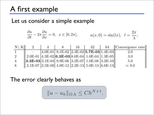
Example 2.4. Consider Eq. (2.1) as
results,
A first example
as . Notewe that observe forseveral N = things. 8, the First, finite the scheme precision is clearly dominates convergentand and dest there
to a converged result; one can increase the local ∂uorder
of ∂uapproximation,
N, and/or
se the number of elements, K.
− 2π =0, x ∈ [0, 2π],
∂t ∂x
Let us consider a simple example
er Eq. (2.1) as
∂u ∂u
− 2π =0, x ∈ [0, 2π],
∂t ∂x
ary conditions and initial condition as
u(x, 0) = sin(lx), l = 2π
λ ,
ength. We use the strong form, Eq. (2.8), although for this simple example, the
ntical results. The nodes are chosen as the Legendre-Gauss-Lobatto nodes as we
il in Chapter 3. An upwind flux is used and a fourth-order explicit Runge-Kutta
to integrate the equations in time with the timestep chosen small enough to
errors can be neglected (See Chapter 3 for details on the implementation).
list a number of results, showing the global L2 with periodic boundary conditions and initial condition as
u(x, 0) = sin(lx), l =
-error at final time T = π as a
ber of elements, K, and the order of the local approximation, N. Inspecting
serve several things. First, the scheme is clearly convergent and there are two
result; one can increase the local order of approximation, N, and/or one can
of elements, K.
2π
λ ,
where λ is the wavelength. We use the strong form, Eq. (2.8), although
weak form yields identical results. The nodes are chosen as the Legendre
shall discuss in detail in Chapter 3. An upwind flux is used and a fourthmethod
is employed to integrate the equations in time with the times
ensure that timestep errors can be neglected (See Chapter 3 for details
In Table 2.1 we list a number of results, showing the global L2-err function of the number of elements, K, and the order of the local ap
these results, we observe several things. First, the scheme is clearly co
roads to a converged result; one can increase the local order of approxi
increase the number of elements, K.
Table 2.1. Global L 2 2.1. Global L
-errors when solving the wave equation using K elem
of approximation, N. Note that for N = 8, the finite precision dominate
convergence rate.
2 -errors when solving the wave equation using K elements each with a lo
roximation, N. Note that for N = 8, the finite precision dominates and destroys the
gence rate.
N\ K 2 4 8 16 32 64 Convergence rate
1 – 4.0E-01 9.1E-02 2.3E-02 5.7E-03 1.4E-03 2.0
2 2.0E-01 4.3E-02 6.3E-03 8.0E-04 1.0E-04 1.3E-05 3.0
4 3.3E-03 3.1E-04 9.9E-06 3.2E-07 1.0E-08 3.3E-10 5.0
8 2.1E-07 2.5E-09 4.8E-12 2.2E-13 5.0E-13 6.6E-13 9.0
e rate by which the results converge are not, however, the same when changing N a
fine h =2π/K as a measure of the size of the local element, we observe that
u − uhΩ,h ≤ Ch N+1 2 4 8 16 32 64 Convergence r
– 4.0E-01 9.1E-02 2.3E-02 5.7E-03 1.4E-03 2.0
2.0E-01 4.3E-02 6.3E-03 8.0E-04 1.0E-04 1.3E-05 3.0
3.3E-03 3.1E-04 9.9E-06 3.2E-07 1.0E-08 3.3E-10 5.0
2.1E-07 2.5E-09 4.8E-12 2.2E-13 5.0E-13 6.6E-13 9.0
asThe a measure error clearly of the behaves size of the as local element, we observe tha
u − uhΩ,h ≤ Ch
.
it is the order of the local approximation that gives the fast convergence rate. The c
es not depend on h, but it may depend on the final time, T , of the solution. To highli
N+1 .
r of the local approximation that gives the fast convergence ra
ich the results converge are not, however, the same when chang
on h, but it may depend on the final time, T , of the solution. T