ChromeGate 3.3.2 Software Manual - KNAUER Advanced Scientific ...
ChromeGate 3.3.2 Software Manual - KNAUER Advanced Scientific ...
ChromeGate 3.3.2 Software Manual - KNAUER Advanced Scientific ...

Create successful ePaper yourself
Turn your PDF publications into a flip-book with our unique Google optimized e-Paper software.
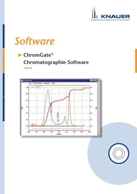
<strong>Software</strong><br />
ChromGate ®<br />
Chromatographie-<strong>Software</strong><br />
V7057-8
CONTENTS 3<br />
CONTENTS<br />
Installation Guide ChromGate ® <strong>3.3.2</strong> ............................................................................... 8<br />
General Definitions .................................................................................................... 8<br />
Installation .................................................................................................................. 8<br />
<strong>KNAUER</strong> FRC control option ...................................................................................11<br />
Short Guide ChromGate ® , <strong>KNAUER</strong> Instrument Control .............................................13<br />
Overview .......................................................................................................................13<br />
Configuring a System ...................................................................................................14<br />
Instrument Configuration .........................................................................................14<br />
System Options .......................................................................................................14<br />
Setting up a Method ......................................................................................................15<br />
The Instrument Wizard ............................................................................................15<br />
The Method Window ................................................................................................16<br />
Quantification of the Compound(s) of Interest ..............................................................19<br />
Overview ..................................................................................................................19<br />
Integration ................................................................................................................19<br />
Generating and Using a Calibration Curve ..............................................................20<br />
Method File Commands ................................................................................................20<br />
Quantification and Using Sequence Files .....................................................................20<br />
Overview ..................................................................................................................20<br />
Single Level Calibration ...........................................................................................21<br />
Creating a Sample Sequence ..................................................................................23<br />
Running a Sequence ...............................................................................................25<br />
Reporting .................................................................................................................26<br />
Collecting Data ..............................................................................................................28<br />
General Data Collection Instructions with ChromGate ............................................28<br />
Collecting Data ........................................................................................................28<br />
Instrument Status of a running Control Method .......................................................29<br />
Shutting Down the System ...........................................................................................30<br />
Setup and Control of Knauer HPLC Systems ...............................................................31<br />
Overview of Instrument Control ....................................................................................31<br />
Configuration – device communication port ............................................................31<br />
Configuring the Interface .........................................................................................31<br />
Knauer Interface Configuration ................................................................................32<br />
Kontron Interface Configuration ...............................................................................34<br />
K-2700 / 2800 Interface Card and Driver Installation ..............................................35<br />
Configuring the <strong>KNAUER</strong> HPLC System .................................................................35<br />
Instrument Configuration ..............................................................................................36<br />
Configuration – <strong>KNAUER</strong> HPLC System .................................................................36<br />
Configuration – Knauer Pumps................................................................................38<br />
Configuration – Kontron Pumps...............................................................................44<br />
Configuration – Knauer Detectors ...........................................................................45<br />
Configuration – User Defined Detectors ..................................................................53<br />
Configuration – Kontron UV-Detectors ....................................................................55<br />
Configuration – Kontron Diode Array Detectors ......................................................56<br />
Configuration – Virtual Detector...............................................................................57<br />
Detector Connections ..............................................................................................57<br />
Configuration – Assistant ASM2.1L .........................................................................60<br />
Configuration – Autosampler ...................................................................................63<br />
Configuration – Autosampler 3950 ...........................................................64
4 CONTENTS<br />
Configuration – Autosampler Knauer Optimas ........................................ 67<br />
Configuration – Autosampler 3800 .......................................................... 70<br />
Configuration – Autosampler 3900 .......................................................... 71<br />
Configuration – Autosampler Triathlon / Endurance ............................... 72<br />
Configuration – Kontron Autosamplers ................................................... 76<br />
Configuration – Miscellaneous Instruments ............................................................ 78<br />
Configuration – Switching Valves ............................................................ 78<br />
Configuration – Manager 5000/5050, IF2 ................................................ 79<br />
Configuration – Column Oven 4050, Column Oven Jetstream ............... 80<br />
Configuration – Flowmeter ...................................................................... 81<br />
Creating an Instrument Control Method ....................................................................... 83<br />
Instrument Setup .......................................................................................................... 84<br />
Instrument Setup – Pumps ..................................................................................... 85<br />
Instrument Setup – Detectors ................................................................................. 91<br />
All Detectors 91<br />
Instrument Setup – RI Detectors ............................................................. 92<br />
Instrument Setup – UV Detectors (S 200, K-200) ................................... 92<br />
Instrument Setup – UV Detectors (K-2000, K-2500) ............................... 92<br />
Instrument Setup – UV Detectors (UVD 2.1L, UVD 2.1S, S 2520, S 2500,<br />
K-2001, K-2501) ............................................. 93<br />
Instrument Setup – Kontron Detectors .................................................... 95<br />
Instrument Setup – K-2600 Detector ....................................................... 95<br />
Instrument Setup – S 2550 Detector ....................................................... 98<br />
Instrument Setup – Diode Array Detectors (S 2600, DAD 2850, DAD<br />
2800, K-2700 and Kontron DAD 540/545) ... 100<br />
Instrument Setup – Fluorescence Detector RF-10Axl / RF-20A ........... 103<br />
Instrument Setup – Alltech 650 Conductivity Detector .......................... 104<br />
Instrument Setup – User defined Detector ............................................ 104<br />
Instrument Setup – Virtual Detector ...................................................... 105<br />
Instrument Setup – Assistant ASM2.1L ................................................................ 107<br />
Instrument Setup – Autosamplers......................................................................... 111<br />
Instrument Setup – Autosampler 3800 .................................................. 111<br />
Instrument Setup – Autosampler Knauer Optimas / 3900 (Midas)........ 112<br />
Instrument Setup – Autosampler 3950 (Alias) ....................................... 116<br />
Instrument Setup – Triathlon/Endurance Autosampler ......................... 121<br />
Instrument Setup – Kontron Autosamplers ........................................... 128<br />
Instrument Setup – Miscellaneous Instruments .................................................... 130<br />
Instrument Setup – Manager 5000/5050/IF2 I/O ................................. 130<br />
Instrument Setup – Switching Valves .................................................... 131<br />
Instrument Setup – Column Oven 4050 ................................................ 133<br />
Instrument Setup – Column Oven Jetstream ........................................ 133<br />
Instrument Setup – Flowmeter .............................................................. 134<br />
Setting up Auxiliary Traces ................................................................................... 135<br />
Setting up a Trigger .............................................................................................. 135<br />
Setting up the Baseline Check .............................................................................. 136<br />
Instrument Status of a (running) Control Method ....................................................... 137<br />
System Status ....................................................................................................... 137<br />
Instrument Status – Pumps ................................................................................... 139<br />
Instrument Status – Detectors .............................................................................. 145<br />
Instrument Status – RI Detectors (S 23[4]00, K-23[4]00/1) ................... 145<br />
Instrument Status – UV Detectors (S 2520, S 2500, S 200, K-200, K-<br />
2000/1, K-2500/1) ......................................... 145<br />
Instrument Status – Kontron Detectors (3xx, 4xx, and 5xx) .................. 147<br />
Instrument Status – fast scanning UV Detector (K-2600) ..................... 148<br />
Instrument Status – Diode Array Detectors ........................................... 149<br />
Instrument Status – Fluorescence Detector RF-10Axl / RF-20A .......... 152<br />
Instrument Status – Conductivity Detector Alltech 650 ......................... 154<br />
Instrument Status – User Defined Detector ........................................... 154
CONTENTS 5<br />
Instrument Status – Virtual Detector ......................................................155<br />
Instrument Status – Assistant ASM2.1L ................................................................156<br />
Instrument Status – Autosampler ..........................................................................161<br />
Instrument Status – Autosampler 3800 ..................................................161<br />
Instrument Status – Autosampler Optimas/3900 ...................................162<br />
Instrument Status – Autosampler 3950 ..................................................163<br />
Instrument Status – Triathlon/Endurance Autosampler .........................165<br />
Instrument Status – Kontron Autosamplers ...........................................166<br />
Instrument Status – Miscellaneous Instruments ....................................................166<br />
Instrument Status – Manager 5000/5050/IF2 I/O ..................................166<br />
Instrument Status – Knauer Switching Valves .......................................167<br />
Instrument Status – Column Oven 4050 and Jetstream ........................168<br />
Instrument Status – Flowmeter ..............................................................169<br />
Knauer Instrument Control Method Options ...............................................................170<br />
General Settings .........................................................................................................170<br />
Runtime Settings ...................................................................................................170<br />
Download Tab / Method .........................................................................................172<br />
Solvent Control ......................................................................................................173<br />
Qualification Procedures .............................................................................................175<br />
Validation of Integration ..............................................................................................178<br />
Generic Drivers ...........................................................................................................183<br />
ChromGate ® System Suitability Setup .........................................................................185<br />
Copy & Paste .........................................................................................................186<br />
Suitability Calculation Selection .............................................................................186<br />
Running a Suitability Test ......................................................................................187<br />
Suitability Reports ..................................................................................................188<br />
ChromGate ® PDA Option...............................................................................................189<br />
PDA Method Setup .....................................................................................................189<br />
PDA Options Library ..............................................................................................189<br />
PDA Options Purity ................................................................................................191<br />
PDA Options Spectrum ..........................................................................................192<br />
PDA Options Multi-Chromatogram ........................................................................194<br />
PDA Options Ratio .................................................................................................195<br />
PDA Views ..................................................................................................................196<br />
3D View ..................................................................................................................196<br />
Contour View .........................................................................................................199<br />
Mixed View.............................................................................................................203<br />
Chromatogram View ..............................................................................................204<br />
Spectrum View .......................................................................................................208<br />
Ratio View ..............................................................................................................210<br />
Spectrum Similarity Table ......................................................................................211<br />
Spectral Library Definition ......................................................................................212<br />
How to Collect Spectra for a Library ......................................................................213<br />
How to Add Spectra to a Library ............................................................................213<br />
Library Search .......................................................................................................214<br />
Spectral Library Search .........................................................................................214<br />
Custom Report ............................................................................................................216<br />
PDA Insert Graph Items .........................................................................................216<br />
PDA Insert Report Items ........................................................................................217<br />
Library Search Report 217<br />
Library Definition Report 218<br />
Spectrum Report 219<br />
Spectral Display 221
6 CONTENTS<br />
Peak Table ................................................................................................................. 221<br />
Analysis Channel .................................................................................................. 222<br />
PDA Analysis and Calculations ................................................................................... 222<br />
Chromatograms Extracted from the 3D Data............................................................. 222<br />
Multi-Chromatogram Channels ............................................................................. 222<br />
Working Chromatogram ........................................................................................ 223<br />
Spectra Extracted from the 3D Data .......................................................................... 223<br />
Analysis Spectra ................................................................................................... 223<br />
Working Spectrum................................................................................................. 223<br />
Background Correction ......................................................................................... 223<br />
Spectrum Interpolation .......................................................................................... 224<br />
Spectrum Smoothing ............................................................................................ 224<br />
Spectrum Derivatives ............................................................................................ 224<br />
Upslope and Down slope Spectra......................................................................... 225<br />
Library Search Calculations ....................................................................................... 225<br />
General ................................................................................................................. 225<br />
Pre-Filters .............................................................................................................. 225<br />
Ratio Chromatogram Calculation ............................................................................... 226<br />
Similarity Calculations ................................................................................................ 226<br />
Lambda Max/Min Calculations ................................................................................... 226<br />
Noise Spectrum Calculations ..................................................................................... 227<br />
Peak Purity Calculations ............................................................................................ 227<br />
Background Correction ......................................................................................... 227<br />
Calculating Total Purity ......................................................................................... 227<br />
Three Point Purity ................................................................................................. 228<br />
Spectrum Export ................................................................................................... 228<br />
PDA Data Export ................................................................................................... 229<br />
ChromGate ® Preparative Option .................................................................................. 230<br />
Fraction Collector Configuration ........................................................................... 230<br />
Virtual Fraction Collector Configuration ................................................. 233<br />
Multi Valve Fraction Collector Configuration ......................................... 234<br />
Fraction Collector Setup ....................................................................................... 235<br />
Fraction Collector Instrument Status..................................................................... 247<br />
Fraction Annotations ............................................................................................. 249<br />
Stacked Injection ................................................................................................... 250<br />
SEC Option .................................................................................................................... 257<br />
Overview .................................................................................................................... 257<br />
SEC Calibration..................................................................................................... 257<br />
Applications of SEC .............................................................................................. 258<br />
Using ChromGate ® SEC <strong>Software</strong> ........................................................................ 258<br />
Running an SEC Calibration Standard ................................................................. 259<br />
Single Run Acquisition ............................................................................................... 260<br />
Defining SEC Baseline .......................................................................................... 263<br />
Defining SEC Result Ranges ................................................................................ 263<br />
Define SEC Peaks ................................................................................................ 263<br />
Annotating SEC Chromatograms.......................................................................... 264<br />
SEC Setup ............................................................................................................ 267<br />
SEC Setup Narrow Standard Method ................................................................... 267<br />
SEC Setup Universal Calibration .......................................................................... 270<br />
SEC Setup Broad Range1 Calibration .................................................................. 273<br />
SEC Setup Broad Range 2 Calibration ................................................................. 275
CONTENTS 7<br />
SEC Custom Reports ............................................................................................278<br />
ChromGate ® SEC Equations .................................................................................281<br />
Typical Wiring Schemes ................................................................................................284<br />
Index ................................................................................................................................291
8 Installation Guide ChromGate® <strong>3.3.2</strong><br />
Installation Guide ChromGate ® <strong>3.3.2</strong><br />
General Definitions<br />
Installation<br />
ChromGate is the Knauer OEM version of the original EZChrom Elite<br />
software from Agilent Technologies. The computers must be running<br />
under Windows 7 Professional or Ultimate 32 bit, Windows Vista<br />
Business or Ultimate 32bit or Windows XP Prof. Service Pack 2 for<br />
EZChrom Elite must be installed. Principally 64 bit or Home versions of<br />
Windows are not supported. The licenses are to be installed on the<br />
enterprise machine. The enterprise machine is also the host of all system<br />
configurations (instruments) and the user and project management data.<br />
A server is the computer that is connected to the HPLC system. A<br />
computer that controls the server in a Client/Server system is called<br />
client. The TCP/IP protocol and Microsoft’s framework .Net version 3 or<br />
higher must be installed on all computers. The TCP/IP protocol can be<br />
installed using the standard procedure with the Windows installation<br />
disks, the .Net version 3 installer can be found on the ChromGate<br />
Installation Disc. For the installation of the ChromGate software, you<br />
must be logged onto the network domain in which you will be working<br />
(only for Client/Server installation) and the person performing the<br />
installation must have administrator rights. All other software, especially<br />
virus detection software, must be shut down.<br />
ChromGate <strong>3.3.2</strong> is shipped on one DVD. It includes the original<br />
EZChrom Elite <strong>3.3.2</strong> from Agilent, the Service Pack 2 of EZChrom Elite<br />
<strong>3.3.2</strong> and the Knauer Add-ons as drivers and additional program options.<br />
The “XXXX” for the ChromGate version is the internal build number (e.g.<br />
1787) and may change if a new build will be released. A new build may<br />
include patches and/or the support of additional devices. The license is<br />
stored on a USB license dongle, labeled with “ChromGate” and the serial<br />
number of the license.<br />
First, EZChrom Elite <strong>3.3.2</strong> must be installed from the “ChromGate<br />
installation Disc”. Click on the link “Install EZChrom Elite <strong>3.3.2</strong> software”<br />
to start the installer. Please refer to the EZChrom Elite installation guide<br />
to install EZChrom Elite.
Installation Guide ChromGate® <strong>3.3.2</strong> 9<br />
Fig. 1 ChromGate installer start window<br />
If EZChrom Elite is installed, after a computer restart, the Service Pack 2<br />
of EZChrom Elite <strong>3.3.2</strong> must be installed. Click on the link “Install Service<br />
Pack 2 for EZChrom Elite <strong>3.3.2</strong>” to start the installer. Finally, ChromGate<br />
as an Add-on for the EZChrom Elite software must be installed. If the<br />
Knauer FRC Option is purchased, the fraction collector drivers and the<br />
advanced fraction collection functionality must be installed with a<br />
separate installer (link “Install <strong>KNAUER</strong> FRC Option”). The Knauer FRC<br />
Option can only be installed, if ChromGate with the same build number<br />
has already been installed.<br />
Do not insert the USB license dongle into the USB port before the<br />
software installation is completed, otherwise the license will not be<br />
recognized.<br />
For all installation work login with administrator access. Before the<br />
installation, switch off all running programs, especially anti-virus<br />
software. In Windows Vista and Windows 7 you must confirm that<br />
the software should be installed. Please also login as administrator<br />
if the computer has rebooted after installation, otherwise the<br />
installation will not be completed.<br />
To install ChromGate, click on the link “Install ChromGate software”.<br />
The components which should be installed can be selected in the next<br />
window. As default, all components which ChromGate supports are<br />
selected.
10 Installation Guide ChromGate® <strong>3.3.2</strong><br />
Fig. 2<br />
Fig. 3<br />
Fig. 4<br />
Click on “Next >” to confirm this window. In the next window click on<br />
“Install” to start the installation. To cancel the installation procedure click<br />
“Cancel”.<br />
The following window will be displayed when the installation has<br />
completed.<br />
Click on “Finish” to finalize the ChromGate installation.
Installation Guide ChromGate® <strong>3.3.2</strong> 11<br />
<strong>KNAUER</strong> FRC control option<br />
Fig. 5<br />
Fig. 6<br />
If you own a fraction collector supported by ChromGate you can install<br />
the <strong>KNAUER</strong> fraction collectors AddOn (<strong>KNAUER</strong> FRC control option).<br />
This option can only be installed if ChromGate v. <strong>3.3.2</strong> is installed. To<br />
control a fraction collector, a <strong>KNAUER</strong> FRC option license must also be<br />
subsequently installed.<br />
Click on “Install <strong>KNAUER</strong> FRC option” to start the installation of the<br />
<strong>KNAUER</strong> FRC control option.<br />
In the next window, the fraction collectors that should be installed can be<br />
selected. As default, all supported fraction collectors will be selected.<br />
Click on “Next >” to confirm the window. In the next window click on<br />
“Install” to start the installation. To cancel the installation procedure click<br />
“Cancel”.
12 Installation Guide ChromGate® <strong>3.3.2</strong><br />
Fig. 7<br />
Fig. 8<br />
The following window will be displayed when the installation has<br />
completed.<br />
Click on “Finish” to finalize the <strong>KNAUER</strong> fraction collectors AddOn<br />
installation.<br />
The installer for the Generic Drivers can be found in<br />
ChromGate\GenericDrivers\Disk1. The installation is only required, if you<br />
wants to control one of the devices, supported via the Generic Driver.<br />
Generic drivers only allow for basic control of devices.<br />
When using a DAD K-2700 or K-2800 with a PCI interface card, the driver<br />
for the interface card must be installed. This driver can be found on the<br />
ChromGate CD in ChromGate\Drivers. If the interface card has been<br />
installed, after a re-start, Windows will ask for the driver.<br />
Start ChromGate once in Demo Mode by clicking Start – All programs –<br />
Chromatography – EZChrom Elite (default settings; refer the EZChrom<br />
Elite installation guide).<br />
Close ChromGate. Insert the USB license dongle into a free USB port of<br />
the enterprise machine. Start ChromGate. The license will be recognized<br />
and can be used.
Short guide ChromGate®, <strong>KNAUER</strong> Instrument Control 13<br />
Short Guide ChromGate ® , <strong>KNAUER</strong> Instrument Control<br />
Overview<br />
This section is provided to assist the operator in the day-to-day operation<br />
of Knauer HPLC systems using ChromGate ® software. It focuses mainly<br />
on routine data acquisition and processing and is to be used in<br />
conjunction with the documentation provided with the ChromGate ®<br />
software and the HPLC system. The full software description can be<br />
found in the online help. The online help will be installed along with the<br />
software. You can open it using the desktop link for the online help or<br />
with the help menu in a ChromGate ® window. Additionally Ii will open in<br />
the context of the currently opened ChromGate ® window, if you press the<br />
key on the computer keyboard.<br />
This chapter assumes that the software has been successfully loaded on<br />
the computer or network and the instrumentation for which it is used has<br />
been installed. It does not include topics that are relevant to installation,<br />
interfacing of the unit to other components of the HPLC system, major<br />
maintenance and other topics that are more properly of interest to the<br />
system administrator. In addition, it is assumed that the chromatographic<br />
conditions for the separation and the overall data processing procedures<br />
are well understood.<br />
The automated operation of the system involves the use of:<br />
� the Method - The method describes instrument control, data<br />
acquisition, data processing, reporting and exporting of data for a<br />
single run. It includes all of the parameters that are used to perform<br />
ad process a run.<br />
� the Sequence - The sequence is a listing of the samples to be<br />
analyzed by the system on an automated basis. The user can select<br />
the method to be used for each analysis.<br />
ChromGate ® includes wizards that lead the user through the generation<br />
of the method and the sequence. In addition, the ChromGate ® software<br />
contains a broad range of features to assist the user and also includes a<br />
number of security options.<br />
This manual is provided to introduce the analyst to the ChromGate<br />
program and provides a discussion of some of the most commonly<br />
performed operations. It is not meant to present a detailed step-by-step<br />
procedure for use of the system or the data processing software.<br />
There are a number of sources for further information, including:<br />
� The Operator <strong>Manual</strong>s and Instruction <strong>Manual</strong>s that are provided<br />
with the modules in the system.<br />
� The documentation provided with ChromGate ® Data System,<br />
particularly the User’s Guide (available on the ChromGate ® -DVD<br />
in EZChrom Elite <strong>3.3.2</strong>\English\<strong>Manual</strong><br />
� Release notes provided with the software (available on the<br />
ChromGate ® -DVD in ChromGate\ChromGate)<br />
� Documentation provided with Microsoft ® Windows ® Configuring the<br />
System
14 Short guide ChromGate®, <strong>KNAUER</strong> Instrument Control<br />
Configuring a System<br />
Instrument Configuration<br />
For more detailed information, please refer to the chapter Instrument<br />
Configuration on page 36. Configuring the system involves the selection<br />
of the instruments and features that are to be used (during installation,<br />
each component of the HPLC system is registered on the network). Once<br />
an instrument configuration has been made it can be easily retrieved.<br />
There are two aspects to system configuration:<br />
� Indicating the modules to be used in a given configuration. As an<br />
example, if the laboratory contains both a Model K-1001 pump and a<br />
K-1800 pump and only the Model K-1001 pump is to be used for a<br />
given separation, setting the instrument configuration includes<br />
selecting this pump and choosing various pump parameters (the<br />
type of pump head that is used, and the desired pressure units).<br />
� Indicating the options that should be used with the method (e.g. if<br />
the baseline check feature should be used).<br />
To generate a new instrument configuration:<br />
� Select File - New - Instrument in the ChromGate ® main window<br />
create a new instrument file, presented by an instrument icon on the<br />
right side of the main window.<br />
� Right click on the instrument icon and select Configure - Instrument<br />
on the context menu that is presented to access the Instrument<br />
Configuration dialog box.<br />
� Verify that the Instrument type field indicates Knauer HPLC system<br />
and press to open the Knauer HPLC dialog box.<br />
� Click on the module that you want to include in the configuration and<br />
press the green arrow to put that icon onto the right-hand side.<br />
Access the Configuration dialog box for a module by double-clicking<br />
on it. The dialog box contains information about the specific module<br />
and lets you edit the configuration information. The configuration<br />
information must match with the configuration of the device. From<br />
devices, which will be controlled via LAN connection, you can readout<br />
the configuration.<br />
� Add and configure all of the modules you want to control, until the<br />
appropriate configuration has been created.<br />
� If additional system options, as SEC, SYS or PDA, are desired,<br />
access the options dialog box by pressing the button. The<br />
purchased options must be enabled to make them accessible in the<br />
instrument. Please refer the next chapter System Options for more<br />
information.<br />
� Once the configuration and desired options have been selected,<br />
press OK to return to the Instrument Configuration dialog box,<br />
indicate the desired name of the instrument and press OK to return<br />
to the main screen.<br />
An existing configuration can be edited by right clicking on the icon for<br />
that configuration and selecting Configure - Instrument. If you alter a<br />
configuration, make sure that you first make a copy of the existing<br />
instrument if you want to maintain both configurations.<br />
System Options<br />
The System Options dialog box is used to access the following:<br />
� System Suitability - used to calculate a number of parameters<br />
pertaining to the overall efficiency of the system such as the<br />
resolution, repeatability, peak asymmetry, number of theoretical
Short guide ChromGate®, <strong>KNAUER</strong> Instrument Control 15<br />
Setting up a Method<br />
plates, noise and drift. A detailed description of the setup of this<br />
feature you can find in the ChromGate ® System Suitability Setup<br />
chapter below.<br />
� SEC - used to calculate a number of parameters for SEC/GPC<br />
related chromatography. It adds special calibration methods and<br />
report options. Please find more in the SEC Option chapter in this<br />
manual and in the original manual EliteSEC, found on the installation<br />
DVD in EZChrom Elite <strong>3.3.2</strong>\English\<strong>Manual</strong>\Optional <strong>Software</strong><br />
<strong>Manual</strong>s.<br />
� PDA - used to calculate a number of parameters that are related to<br />
the use of photodiode array detection. A detailed discussion of this<br />
feature is presented in the chapters ChromGate ® PDA Option<br />
starting on page 185 and PDA Analysis and Calculations on page<br />
222. The original software manual PDA Analysis can be found on<br />
the installation DVD in EZChrom Elite <strong>3.3.2</strong>\English\<strong>Manual</strong>\Optional<br />
<strong>Software</strong> <strong>Manual</strong>s.<br />
� Baseline Check - used to verify that the baseline is stable enough to<br />
provide useful chromatograms. A detailed discussion of this feature<br />
is presented in the chapter Setting up the Baseline Check on page<br />
136.<br />
A method is a set of parameters that describes the instrumental<br />
conditions for a chromatographic separation and includes information<br />
about data processing and reporting. It includes the parameters for the<br />
operation of each of the various modules in the HPLC system such as the<br />
pumps, detectors, oven and the autosampler, which are downloaded to<br />
the various modules for use when the separation run is initiated.<br />
The Method window is used to set up a method, and is accessed via the<br />
Method wizard. The Method window includes a tab for each component<br />
of the system, and the tab presents various parameters that are available<br />
via the control panel of that module. The various tabs that are presented<br />
in the Method window are described in the chapter The Method<br />
Window.<br />
Method files can be saved (*.met) and retrieved as well as imported from<br />
or exported to another instrument in the same manner as other Windows<br />
files. Please note, that for devices, which are not configured in the<br />
original instrument, the parameters will be set to default values.<br />
The Instrument Wizard<br />
The Instrument Wizard is used to lead you through the steps required to<br />
create a new method or modify an existing one, create a new sequence<br />
or run a method or sequence. The Instrument Wizard will always start, if<br />
you open an instrument. You can also start it from the opened instrument<br />
window with a click on the Wizard icon.
16 Short guide ChromGate®, <strong>KNAUER</strong> Instrument Control<br />
Fig. 9 Instrument Wizard<br />
Select Create or modify a method to bring up the method window:<br />
Fig. 10 Method Wizard<br />
Click the appropriate button to present the Method window, which can be<br />
edited as described in the section The Method Window.<br />
If you are more familiar with the menus, you can ignore the wizard. If you<br />
don’t want to start the Wizard always if you open the instrument, disable<br />
the checkbox “Show at instrument startup”.<br />
The Method Window<br />
Overview<br />
The Method window includes a tab for each instrument in the system on<br />
which you can select the particular run parameters. The information on a<br />
given tab is essentially the same as if you were to program the<br />
component on a standalone basis. The reader should review information<br />
about parameter selection that is provided in the instruction manual for<br />
each module.<br />
Pump Tabs<br />
The Pump tab contains several areas where you can enter parameters<br />
related to operating mode, control pressure limits, and flow programs.<br />
The tab for the Smartline Pump 1000 is presented below (the tabs for<br />
other pumps are very similar).
Short guide ChromGate®, <strong>KNAUER</strong> Instrument Control 17<br />
Fig. 11 Instrument setup tab (Smartline Pump 1000)<br />
Details for the Control Settings, Control Pressure Limits as well as the<br />
creation of a Time Table are described in the section Instrument Setup –<br />
Pumps on page 84.<br />
Detector Tabs<br />
The format of the detector tab is dependent on the nature of the specific<br />
detector. A typical tab is shown below. Some of the parameters are<br />
common to essentially all detectors and are described at the beginning of<br />
the chapter Instrument Setup – Detectors on page 89, followed by details<br />
which are specific to certain detectors:<br />
RI Detectors (S 23[4]00, K-23[4]00/1) ............................................ page 92<br />
UV Detectors (S 200, K-200) ......................................................... page 92<br />
UV Detectors (K-2000, K-2500) .................................................... page 92<br />
UV Detectors (S 2500, K-2001, K-2501, UVD2.1S) ...................... page 93<br />
Instrument Setup – Kontron Detectors .......................................... page 95<br />
K-2600 Detector…………. .............................................................. page 95<br />
UV Detectors S 2550 / S 2520……………………………………….. page 80<br />
Diode Array Detectors (S 2600, K-2700, DAD 2800/2850 and<br />
Kontron DAD 540) .............................. page 100<br />
Fluorescence Detector RF-10Axl / RF-20A/Axs .......................... page 103<br />
Instrument Setup – Alltech 650 Conductivity Detector ................. page 104<br />
User defined Detector…………………………………………… ..... page 104<br />
Instrument Setup – Virtual Detector ............................................ page 105
18 Short guide ChromGate®, <strong>KNAUER</strong> Instrument Control<br />
Fig. 12 UV Detector S 2600 tab<br />
Autosampler Tabs<br />
Different autosamplers can be controlled by the ChromGate ® software.<br />
Any method window will include the tab for the configured one, to setup<br />
the needed injection parameters. You will find detailed setup information<br />
for the autosamplers starting on page 111.<br />
Fraction Collector Tabs<br />
Several fraction collectors including the Knauer multi valve FC and a<br />
virtual one can be controlled by the ChromGate ® software. Any method<br />
window will include the tab for the configured one, to setup the needed<br />
control parameters. You will find detailed setup information for the<br />
fraction collectors on page 235.<br />
Miscellaneous Instrument Tabs<br />
Further instruments to be controlled by this software are:<br />
Manager 5000/5050, IF2 (analog/digital outputs of the Knauer A/D<br />
converters<br />
Knauer Switching Valves<br />
Valco Switching Valves<br />
Column oven 4050, Jetstream oven<br />
Flowmeter<br />
For each of them a tab will be shown in the method window as far as the<br />
instrument has been configured. If you have included more the one of the<br />
Knauer or Valco Switching Valves from one configuration window, even if<br />
they are of different type (K-6, K-12, or K-16) they are represented<br />
together in one tab. The detailed description is given on page 131.<br />
Baseline Check tab<br />
The Baseline Check tab is presented if Baseline Check is selected on the<br />
Configuration Options dialog box (see section Setting up the Baseline<br />
Check on page 136). It is used to ensure that the baseline is satisfactory.<br />
The Baseline check must be enabled in the Options menu of the<br />
instrument configuration.
Short guide ChromGate®, <strong>KNAUER</strong> Instrument Control 19<br />
To use this feature, select the Baseline Check option in the Single<br />
Run dialog box or include Baseline Check in the current Sequence<br />
line.<br />
When the baseline feature is selected, the initial conditions for the run will<br />
be used to acquire baseline data. If the data is satisfactory for all<br />
channels, the run will be performed; if the baseline data is not<br />
satisfactory, the run will be aborted and a message to that effect will be<br />
presented.<br />
Trigger tab<br />
The Trigger tab is used to indicate the action to start a chromatogram.<br />
The definition of the various options is presented on the tab. For details<br />
see page 135.<br />
Quantification of the Compound(s) of Interest<br />
Overview<br />
Integration<br />
The change of the signal from a detector is related to the concentration of<br />
the eluting compound. Under ideal circumstances, the peak for each<br />
compound of interest will be well-resolved from other peaks in the sample<br />
and will be a Gaussian peak. In this case, the area of the peak is directly<br />
related to the concentration of the compound of interest. The analyst<br />
could generate a calibration plot using standards of known concentration<br />
to determine the concentration/area relationship, and then use the<br />
calibration plot to determine the concentration of unknowns.<br />
The calibration data is incorporated into the method, so that when you<br />
select a method to use, all of the information that is required for<br />
quantization is loaded.<br />
Integration of the chromatogram requires two basic parameters, the<br />
width and the threshold, which define the starting point and ending point<br />
for a peak and to distinguish a peak from noise. When a method is<br />
established, the default values are entered, and these can be edited via<br />
the Integration Events window which is accessed by selecting<br />
Method/Integration Events.<br />
Fig. 13 Integration Events window<br />
The Width value is used to calculate a value for bunching or smoothing<br />
the data points before the integration algorithm is applied integration<br />
works best when 20 points are sampled across a peak. The width should<br />
be selected for the narrowest peak in the chromatogram.<br />
The Threshold value is the first derivative of the chromatogram, and is<br />
used to distinguish the peak from noise and/or drift.<br />
To set the noise and drift, select the desired event field, then select the<br />
start and stop time and value.<br />
ChromGate ® includes a large number of additional parameters that can<br />
be used to refine the chromatogram. These can be applied on a<br />
programmed basis or on a manual basis for data that is already collected.<br />
A detailed discussion on integration is presented in the ChromGate ®<br />
Chromatography Data System, Reference <strong>Manual</strong>.
20 Short guide ChromGate®, <strong>KNAUER</strong> Instrument Control<br />
Generating and Using a Calibration Curve<br />
A calibration curve is normally generated via a sequence, which is<br />
discussed in the chapter Quantitation and Using Sequence Files below.<br />
Method File Commands<br />
A method file can be saved, retrieved and edited as desired in the same<br />
way as with other Windows applications. As an example, if the Method<br />
dialog box is open and you want to save a new method, select<br />
File/Method/Save as and enter the desired name.<br />
Fig. 14 Save Method File as… Window<br />
Similarly, if you want to open a method, select File/Method/Open… and<br />
enter the file name.<br />
A printed report describing all aspects of a method can be obtained by<br />
selecting File/Method/Print.<br />
Quantification and Using Sequence Files<br />
Overview<br />
Calibration involves the generation of the relationship between the<br />
concentration of a compound and the area of the corresponding peak in<br />
the chromatogram. Once calibration is established, it can be used to<br />
determine the concentration of the compound of interest in unknowns.<br />
A single level calibration involves a single sample to calculate the<br />
calibration constant; the curve is generated from that point and the origin.<br />
A multi-level calibration uses several standards (e.g. 10 µg/ml, 20 µg/ml,<br />
50 µg/ml, 100 µg/ml).<br />
Setting up a calibration involves the following steps:<br />
1. Run the chromatograms containing the standards and<br />
save them<br />
2. Identify the peaks from the standards<br />
3. Generate a peak table<br />
4. Generate the standard curve<br />
The standards used to generate a calibration should be well defined and<br />
should be in a matrix that is similar to that containing the samples that<br />
you will analyze. The standards undergo exactly the same sample<br />
preparation process that is used for real samples.
Short guide ChromGate®, <strong>KNAUER</strong> Instrument Control 21<br />
There are two general ways that a standard can be employed:<br />
� Internal Standard - A known amount of the compound used as a<br />
standard is added to the sample, and the area for the compound of<br />
interest is compared to the area of the standard.<br />
� External Standard - The standard is a separate sample and the<br />
observed intensity is used to generate the calibration curve directly.<br />
The application program allows you to generate calibration curves for a<br />
number of compounds in a single operation and an analytical report can<br />
be generated, printed and exported as desired.<br />
Single Level Calibration<br />
To set up a single level calibration:<br />
1. Collect a chromatogram containing the standard and save it. The<br />
concentration of the compound in the standard should be similar to<br />
that in the samples that you want to analyze.<br />
2. Open the stored data file<br />
3. Press the Analyze button to integrate the chromatogram and<br />
show the baseline.<br />
4. Press the Define Single Peak button to present the Define<br />
Single Peak dialog box. The retention time in the upper right corner<br />
will refer to the first peak in the chromatogram.<br />
Fig. 15 Single peak definition<br />
5. Press the Next>> button until the peak corresponding to the<br />
standard is selected. As an alternative, you can simply click on the<br />
peak in the chromatogram with the cursor.<br />
6. Complete the dialog box for the first standard:<br />
- Enter the peak name<br />
- Indicate the concentration level. For a single level<br />
concentration, enter 1 for the level and indicate the<br />
concentration of the standard.<br />
- Indicate the desired unit (e.g. µg/ml)<br />
- Enter the internal standard ID# if you are using the internal<br />
standard method. This number is obtained from the peak table.<br />
Leave it blank until you have generated the peak table (see<br />
below), then enter the value directly into the Peaks / Groups<br />
table.
22 Short guide ChromGate®, <strong>KNAUER</strong> Instrument Control<br />
Fig. 16 Peak table<br />
- Enter the Reference ID#, which is the Peak ID#s from the peak<br />
table. This number is obtained from the Peak Table. Leave it<br />
blank until you have generated the peak table, then enter the<br />
value directly into the Peaks / Groups table.<br />
- Indicate the desired basis for the calculation of the retention<br />
time window and the desired value.<br />
7. Repeat the above step for each compound in the standard. When<br />
you have entered information for all standards, press Done.<br />
8. Press the Peaks / Groups Table button or select the menu<br />
sequence Method – Peaks / Groups … to present the calibration<br />
peak table. Each peak that you have defined will appear as a row<br />
in the table, along with the retention time and other parameters that<br />
you have entered.<br />
9. Enter all values needed for the calibration as the concentration for<br />
all levels of your compounds.<br />
10. If the table is complete, close Peak Table dialog box by clicking on<br />
the x in the upper right corner.<br />
11. Save the method.<br />
12. Select Analysis/Analysis Single Level Calibration from the<br />
menu bar to present the following dialog box.<br />
Fig. 17 Analysis Single Level Calibration Window<br />
13. Enter the sample identification used for the standard.<br />
14. Enter the method that you want to calibrate and the data path<br />
name for the data file.<br />
15. Enter the name of the calibration data file.<br />
16. Click on the Calibration check box and enter a 1 for Calibration<br />
level. If the method is presently not calibrated, it is not necessary to<br />
check any of the boxes (but if you want to be certain, select the<br />
Clear all calibration check box).<br />
17. Repeat the steps 12. to 16. for all levels you want to calibrate.<br />
Enter the appropriate calibration level into the Calibration level field
Short guide ChromGate®, <strong>KNAUER</strong> Instrument Control 23<br />
18. Click Start. The peaks will be integrated, and calibration curves will<br />
be generated.<br />
The method is now calibrated and can be used to analyze samples.<br />
Creating a Sample Sequence<br />
If you are using an autosampler, the sequence is used to define the<br />
samples, indicate how they are to be injected, the method used to<br />
separate them and how the data is to be calculated. A sample sequence<br />
can be used to acquire both calibration data as well as data from<br />
unknowns (and both can be performed in a single sequence). In addition,<br />
a sequence is used to generate a calibration curve and analyze<br />
unknowns from stored data.<br />
To setup a sequence:<br />
1. Click File/Sequence/Sequence Wizard or select Create a<br />
Sequence on the Instrument Wizard to access the Method page of<br />
the Sequence wizard.<br />
Fig. 18 Sequence Wizard – Method<br />
2. Enter the method name<br />
3. Select the mode of data acquisition. If the data is to be collected as<br />
part of the sequence, the Amount Values fields will be activated.<br />
When you are beginning to develop a sequence, ignore them and<br />
press Next to present the Sequence Wizard –Unknowns. If the From<br />
existing data files option is selected, a dialog box will be presented<br />
to select the desired files.
24 Short guide ChromGate®, <strong>KNAUER</strong> Instrument Control<br />
Fig. 19 Sequence Wizard –Unknowns<br />
4. Press the blue arrow on the Sample ID line to access a list of<br />
identification options for the samples. Typically, Line Number and<br />
Method Name are used, so that each sample will be identified with<br />
the sequence line number and method name.<br />
5. Indicate where the data should be stored using the Data Path field.<br />
6. Click on the blue arrow on the Data File line to access how the data<br />
file should be named. Typically Sample ID is used, this will assure<br />
that the sample is uniquely identified and easily related to the<br />
sample.<br />
7. Enter the appropriate number of unknowns the number of<br />
repetitions.<br />
8. Press next to present the Autosampler screen if you have indicated<br />
that the data files are to be acquired (initial screen in the wizard).<br />
(this screen is not presented if existing data files are used).<br />
Fig. 20 Sequence Wizard – Autosampler<br />
9. Enter the appropriate information and press Next to present:
Short guide ChromGate®, <strong>KNAUER</strong> Instrument Control 25<br />
Fig. 21 Sequence Wizard – Calibration<br />
10. Enter the desired information and press Next to access the Reports<br />
page.<br />
Fig. 22 Sequence Wizard – Reports<br />
11. Enter the desired information and press Finish to present a<br />
spreadsheet that describes the overall sequence.<br />
Fig. 23 Sequence Wizard –Description of a finished sequence<br />
12. Save the sequence.<br />
Running a Sequence<br />
To acquire data using the sequence file you just created, click the<br />
Sequence Run button on the command ribbon, or do a right-hand mouse<br />
click in the sequence spreadsheet, and select Run Sequence. The<br />
following dialog box will appear:
26 Short guide ChromGate®, <strong>KNAUER</strong> Instrument Control<br />
Fig. 24 Run Sequence dialog box<br />
Reporting<br />
Enter the name of your sequence file by typing the name, along with<br />
path, in the Sequence Name field. You can also select it from a list of<br />
sequence files on your disk by clicking the File button next to the field.<br />
Leave the other parameters as their defaults.<br />
Prepare your autosampler to inject your standard sample, followed by 3<br />
unknown samples. When you are ready to inject your first sample, click<br />
Start. When the sequence is completed, you will have acquired and<br />
saved the data files for one standard and three unknown runs, and<br />
generated a simple result report for each unknown sample and a<br />
summary report for the sequence.<br />
Since you have not yet defined a sequence summary report, do not<br />
check the box to print sequence reports.<br />
ChromGate ® Client/Server comes with a complete suite of report<br />
templates that can be used without modification to generate reports. To<br />
see an example of one of these reports, use the Reports/View/Area%<br />
command from the menu bar. (Make sure your current chromatogram<br />
has been analyzed first.) The standard report will appear in a window on<br />
your screen.<br />
Fig. 25 Area% Report<br />
If your method contains no defined custom report, the system will use the<br />
standard report formats to print reports when required.
Short guide ChromGate®, <strong>KNAUER</strong> Instrument Control 27<br />
Knauer has added three reports in a fresh design (Knauer Area%<br />
Report, Knauer ESTD Report, Knauer ISTD Report), which also can be<br />
found as standard reports in the Report menu.<br />
Fig. 26 <strong>KNAUER</strong> Area% Report<br />
If you wish, you can modify the standard report templates, or create<br />
entirely new reports using the Custom Report capability of ChromGate ®<br />
Client/Server. Modified standard reports can be stored as templates,<br />
Custom Reports will be available as part of the method. You can create<br />
custom method reports and / or custom Sequence reports.<br />
To view the custom report template in the multilevel calibration.met file,<br />
first open the file if it is not already open. (Use the File Open button,<br />
followed by Method; then select the template from the file list.) Click the<br />
Edit Custom Report button on the command toolbar to access the<br />
method custom report editor. The current method custom report template<br />
will appear.
28 Short guide ChromGate®, <strong>KNAUER</strong> Instrument Control<br />
Collecting Data<br />
General Data Collection Instructions with ChromGate<br />
The user should review the operating manual for each component in<br />
the system for warm up requirements, preparing the component for<br />
operation, etc.<br />
This section includes requirements and suggestions relative to the<br />
computer and e-line network when ChromGate ® is used to operate the<br />
HPLC system.<br />
Before starting the chromatographic runs:<br />
� Make sure that the energy saving feature and the screen saver<br />
on the computer are off.<br />
� Check that all modules are connected to the e-line cable<br />
� To power up the system, first turn on the PC and finally power up<br />
the various modules.<br />
If a unit loses power or if the communication is broken, turn off all<br />
components and start over.<br />
Collecting Data<br />
� If a module has been operating via the local mode (UI interface),<br />
make sure that it is not in use when connecting the cable.<br />
� If you are using a manual injector, make sure that the system is<br />
in the waiting for injection mode waiting for trigger before<br />
injecting.<br />
� If you are using an autosampler with a single rack, the input<br />
numbers should be integers. If you are using multiple racks, input<br />
vial numbers, using a letter and number (e.g. A1, B3, etc.) should<br />
be used. If an incorrect vial number or invalid volume is noted,<br />
the sequence will stop.<br />
When you want to collect data, click on the desired instrument to present<br />
the Instrument Wizard dialog box (Fig. 9 on page 16) and select the<br />
desired operation.<br />
If you select Run one sample, the Single Run Acquisition dialog box will<br />
be presented. Enter the desired Sample ID, method and name (e.g.<br />
sample.dat) and then press Start.<br />
The chromatogram will be collected as described in the method. During<br />
the data acquisition, the chromatogram will appear in the window as<br />
shown below.
Short guide ChromGate®, <strong>KNAUER</strong> Instrument Control 29<br />
Fig. 27 Single run data acquisition window<br />
If you have selected Run a sequence of Samples, the following dialog<br />
box will be presented:<br />
Fig. 28 Sequence Run Acquisition dialog box<br />
Enter the Sequence name and press Start. The chromatogram for the<br />
first run will be collected when the conditions have been met.<br />
Instrument Status of a running Control Method<br />
During Data acquisition, you can access the status of the system by<br />
selecting Control/Instrument Status on the main menu. The window that<br />
will be presented is shown below, and the format and tabs is dependent<br />
on the configuration of the system.<br />
Open the Instrument Status Window using the menu sequence Control –<br />
Instrument Status.<br />
The Instrument Status window contains the status tabs for all configured<br />
instruments, and as shown in the figure below the system status tab,<br />
providing an overview for the whole system.
30 Short guide ChromGate®, <strong>KNAUER</strong> Instrument Control<br />
Fig. 29 Instrument Status window, system status tab of a running method<br />
The running method is visualized by the dark dotted lines between the<br />
displayed instruments.<br />
For each pump, identified by name and serial number, the actual flow,<br />
pressure is displayed. If a gradient system is configured the solvent<br />
composition also will be shown.<br />
For each detector channel the wavelength and output values are shown.<br />
Similarly for all included instruments the relevant data will be displayed,<br />
e.g. the actual switching positions in case of the valves.<br />
All these information you also find on the single instrument tabs of this<br />
window, for details see pages 139 - 169. On these tabs you get the<br />
possibility of direct control interaction with the individual instruments. This<br />
is even possible during a method is running; however this option must be<br />
enabled while configuring the system (refer to Knauer instrument control<br />
method options on page 170).<br />
Shutting Down the System<br />
The system can be automatically shut down at the end of a sequence by<br />
including a shutdown method at the end of a sequence. A discussion of<br />
sequence types is presented in Chapter 4 of the reference manual.<br />
The shutdown method should include the following;<br />
� Column Oven temperature – value should be below ambient<br />
� Pump conditions, the flow for all pumps should be 0.0 ml/min and<br />
100% A and no events. For new pumps as Smartline pump 1050<br />
also a Standby option is available.<br />
� Deselect any timed events and Mix methods.<br />
� Set the Trigger to None. Now an autosampler will not be<br />
controlled and will not perform an injection.<br />
� Detector – activate the Lamp Off option or, if supported, the<br />
Standby option.
Setup and Control of Knauer HPLC Systems 31<br />
Setup and Control of Knauer HPLC Systems<br />
This manual contains detailed information on the use of the ChromGate ®<br />
instrument control software option for the Knauer Instruments.<br />
It contains information on how to configure, set up and run samples<br />
automatically from the ChromGate ® Chromatography Data System.<br />
This manual is intended to be a supplement to the general ChromGate ®<br />
Data System documentation and contains information specific to the use<br />
of the optional instrument control software.<br />
Overview of Instrument Control<br />
The instrument control software for the Knauer HPLC System enables<br />
you to enter instrument control parameters that become part of the<br />
method. The parameters are then executed in real time when samples<br />
are acquired using the data system. The software allows you to set and<br />
control parameters as pressures, flows and gradients for pumps,<br />
wavelengths and scans for detectors, injection parameters for<br />
autosamplers on the Knauer HPLC System, and monitor these in realtime.<br />
Configuration – device communication port<br />
Some of the devices have two communication ports on the rear panel for<br />
controlling the device by the computer. One is an RS-232 port, also<br />
called serial or COM port; the other is an Ethernet port, also called LAN<br />
(Local Area Network). Beside the Knauer valve drives, for all the devices<br />
the desired communication port must be defined in the device. Please<br />
pay attention to the corresponding notes in this manual and refer to the<br />
device’s manual for more information, how the desired communication<br />
port must be configured. Please note, that for some devices the<br />
functionality depends on the selected communication port.<br />
Configuring the Interface<br />
Beside all detectors directly supported in ChromGate ®<br />
, any detector or<br />
sensor producing an analog signal which can be digitized with an A/D<br />
converter or Interface Box can be used for data acquisition. You must<br />
configure your data acquisition interface before you can acquire analog<br />
data using the data system. The Knauer interfaces can also be used to<br />
control other devices by analog or digital output.<br />
Interface configuration is accessed through the Tools command on the<br />
ChromGate Main Menu.<br />
Click the Tools - Interface Configuration command from the<br />
ChromGate ® Main Menu. A window will appear displaying several<br />
possible interface devices. To configure a device, click on the icon to<br />
select it, then click the button or double click on the<br />
instrument icon.
32 Setup and Control of Knauer HPLC Systems<br />
Fig. 30 Selection window for interface configurations<br />
Knauer Interface Configuration<br />
If you are using either a Knauer Interface Box/IF2 or a Manager<br />
5000/5050, click on the corresponding icon, and then click Properties. A<br />
dialog box will appear where you can configure the Interface Box (see<br />
Fig. 32).<br />
In regards to Knauer software, the Manager 5050 interface module is<br />
identical to the Manager 5000. To configure the Manager 5050,<br />
please select „Manager 5000“.<br />
If you configure the interface newly, the message like Fig. 31 will remind<br />
you to enter the serial number of the interface device.<br />
Fig. 31 Error message for missing serial number<br />
Click OK and perform the required settings. The same message will<br />
appear if you try to close the setup window without an entered serial<br />
number.<br />
Fig. 32 Dialog box for configuring the Manager 5000/5050<br />
The Knauer Interface Box and the Manager 5000/5050 require the same<br />
parameters to be set up. Therefore, the configuration dialogs for both<br />
devices are nearly identical.
Setup and Control of Knauer HPLC Systems 33<br />
Number of boxes<br />
Select the number of boxes used in the system. ChromGate ® supports up<br />
to 4 Knauer Interface Boxes.<br />
Configure box #<br />
Select the box you wish to configure. Each box has to be configured<br />
separately.<br />
Serial Port<br />
Manager 5000/5050 / Interface Box IF2<br />
Select the number for the communication port on your PC to which<br />
the Manager 5000/5050 or the Interface Box IF2 is connected.<br />
Interface Box Model 96<br />
The Knauer Interface Box supports the binary Knauer Net. The<br />
networks 1, 2,... correspond to the number of the utilized<br />
communication port (COM1, COM2,...). Select the number for the<br />
communication port on your PC to which the Interface Box is<br />
connected.<br />
You can use the Interface Box or the Manager 5000/5050 to acquire<br />
signals from different instruments at the same time. It is necessary<br />
to connect the interfaces to separate communication ports on a PC.<br />
See the Typical Cabling / Wiring chapter, Fig. 389 on page 285.<br />
Serial Number<br />
Type in the serial number of the Interface Box / Manager 5000/5050 you<br />
are using. The serial number is used for the device identification and<br />
addressing during serial communications. This serial number should<br />
match the serial number of the Interface Box. For Knauer HPLC-Boxes<br />
with an S/N higher than 65000, only the last 4 digits of the S/N must be<br />
entered (e.g. 5567 instead of 65567).<br />
Box type<br />
The only choice is Model 96. No others are selectable.<br />
Channel<br />
Four data acquisition channels are normally available. However, only<br />
channel one will be available if you have checked the 100 Hz sampling<br />
rate option in model 96 or 50 Hz in case of Manager 5000/5050 / IF2 (see<br />
Sampling rate on page 91).<br />
Fig. 33 Dialog box for configuring the Model 96 Interface Box with activated<br />
100 Hz option<br />
Range<br />
Select the Signal Range for the channel chosen from the channel dropdown<br />
list. The choices are +/-10 V, +/-1 V, +/-0.1 V, +/-0.01 V for the<br />
Interface Box and +/-2.56 V, +/-1.28 V, +/-0.64 V, +/-0.16 V for the<br />
Manager 5000/5050 / IF2. The Signal Range specifies the maximum
34 Setup and Control of Knauer HPLC Systems<br />
analog input voltage to be digitized by an A/D converter. Use the Signal<br />
Range to optimize the signal-to-noise ratio of the measured signal.<br />
Manufacturer and Model<br />
This area is for information only. It contains manufacturing information<br />
about the box which may be required in service situations.<br />
Kontron Interface Configuration<br />
If you are using a Kontron interface card click on the corresponding icon,<br />
and then click Properties. A dialog box will appear where you can<br />
configure the interface (see Fig. 34).<br />
If you configure the interface newly the message like Fig. 31 on page 32<br />
will remind you to enter the serial number of the interface device.<br />
Fig. 34 Dialog box for configuring the Kontron interface card PCI AD<br />
Number of PC cards<br />
Select the number of PC cards used in the system. ChromGate ® supports<br />
up to 4 interfaces.<br />
Configure card #<br />
Select the card you wish to configure. Each card has to be configured<br />
separately.<br />
Card type:<br />
Select either ISA AD or PCI AD. In case of selected PCI AD the setup<br />
window is changed to the following appearance.<br />
Fig. 35 Dialog box for configuring the Kontron interface card ISA AD
Setup and Control of Knauer HPLC Systems 35<br />
K-2700 / 2800 Interface Card and Driver Installation<br />
ChromGate ® communicates with the Diode Array Detectors K-2700 and<br />
2800 via either a PCI interface card or LAN. Installation of the necessary<br />
PCI card is described in the detector manual. Please note, that the driver<br />
is not released for Windows Vista or Windows 7. For other PDA detectors<br />
(S 2800, S 2850…) only the LAN interface will work.<br />
Configuring the <strong>KNAUER</strong> HPLC System<br />
In order to access commands for control of Knauer instruments and<br />
autosamplers, you must configure them appropriately. To access the<br />
configuration screens, locate the icon on the main menu for the<br />
instrument you want to configure.<br />
You must have system administration privileges in order to<br />
configure an instrument.<br />
Fig. 36 ChromGate® main screen<br />
Select File – New to create new instruments or groups:<br />
Fig. 37 Creating new Instrument or Location/Group<br />
If you have selected Instrument, the Instrument Configuration dialog<br />
(see Fig. 38) appears. For already existing instruments right- mouse click<br />
on the instrument, and select the Configure… command.<br />
The Instrument Configuration dialog will appear.
36 Setup and Control of Knauer HPLC Systems<br />
Fig. 38 Instrument configuration dialog box<br />
Instrument name<br />
Enter a descriptive name by which the instrument is identified. This name<br />
will appear under the instrument icon, and when the instrument window is<br />
displayed.<br />
Instrument type<br />
Select the Instrument type from the drop-down list. Knauer devices are<br />
only available in the Knauer HPLC system type<br />
Server name (in Client/Server only)<br />
Select the Server name. This is the name of the CG server to which the<br />
instrument is attached.<br />
Finally, click on Configure to proceed to the instrument configuration<br />
where one can define the detectors, pumps, and further devices for the<br />
instrument.<br />
Instrument Configuration<br />
Configuration – <strong>KNAUER</strong> HPLC System<br />
When you click the Configure button, the following dialog will appear.<br />
Fig. 39 Instrument selection window<br />
Several icons will be displayed in the Available Modules box on the left.<br />
Add modules to be configured by double-clicking on each, or by clicking<br />
once on the icon, followed by the green arrow.
Setup and Control of Knauer HPLC Systems 37<br />
Fig. 40 Instrument selection window with selected items<br />
Auto Configuration<br />
Using the Auto Configuration button, all devices, connected via LAN<br />
and switched on, will be automatically added and configured.<br />
Fig. 41 Auto Configuration start window<br />
All Knauer devices use a single IP port for LAN communication. Only<br />
devices with the same IP port as selected in the Auto Configuration<br />
window will be found. The default IP address is 10001. It can be changed<br />
manually in the device’s setup.<br />
We recommend reviewing the configuration of all automatically added<br />
devices. Devices connected via RS-232 (serial connection) will not be<br />
found and must be added manually.<br />
Now configure or review each module (detector, pump, autosampler, or<br />
event configuration) separately. Not configured instruments may be<br />
indicated by a question mark on the corresponding icons. If you try to exit<br />
the window with OK and one or more instruments are still not configured,<br />
a message like Fig. 42 will appear.<br />
Fig. 42 Example of an operation message to complete configuration<br />
Options<br />
The Options button is used to initiate any optional analysis software for<br />
this instrument.
38 Setup and Control of Knauer HPLC Systems<br />
A list of available analysis options will be presented.<br />
Fig. 43 analysis options window<br />
Click the box(es) to select the optional software you want to enable for<br />
this instrument. The additional licenses are required beside the Baseline<br />
Check. For more information regarding the option, please check the<br />
System Options part above on page 14. The Knauer Fraction Collectors<br />
Control option (FRC) must not been enabled here. Whenever a<br />
configuration with a fraction collector is started, an installed FRC license<br />
will be activated.<br />
Configuration – Knauer Pumps<br />
For each pump in the Configured Modules window, double-click the icon<br />
and complete the configuration dialog.<br />
For configuration information regarding the PLATINblue pump P-1,<br />
please refer to the PLATINblue system manual.<br />
If the pump S 1050 should be controlled by RS-232, in the pump’s<br />
own setup the “Interface” must be set to “RS232 115200”. Please<br />
refer to the pump’s manual, chapter “Setup menu” for more<br />
information.<br />
The pumps K-1000, K-1001, S 1000 and K-1800 (preparative pump<br />
1800) only can be controlled with ChromGate, if the pump’s internal<br />
communication in the menu option “CONTROL” is set to “NET baud<br />
rate 9600”.<br />
To control a pump K-501, in the pump’s internal setup the menu<br />
option “CONTROL” must be set to “Ext:RS232”. The firmware<br />
version must be v. 1.23 or higher.<br />
If you are operating a K-1001 pump fitted with a firmware version<br />
< 5.x, you must select the K-1000 icon for configuration. This is due<br />
to the status information, which the older firmware does not<br />
support. Otherwise you will get error messages when the pump<br />
starts running. For those pumps no advanced status information<br />
and no pressure trace recording are available.
Setup and Control of Knauer HPLC Systems 39<br />
Fig. 44 Pump S 1000 configuration window<br />
Fig. 45 Pump 10P/20P/P2.1S/P4.1S configuration window<br />
Fig. 46 Pump S 1050 configuration window<br />
Fig. 47 Pump P2.1L configuration window<br />
The configuration windows for the other Knauer pumps are nearly<br />
identical.
40 Setup and Control of Knauer HPLC Systems<br />
Name<br />
The name of the selected pump appears automatically. You can enter<br />
any other descriptive name for the pump. This name will appear on the<br />
pump tab when the instrument setup or status windows are displayed.<br />
Use a name which is unique within the instrument (configuration).<br />
E.g. for a high-pressure gradient system, all pumps must have<br />
different names.<br />
Pump Type (accessible for Pump K-120/501 only)<br />
Select the type of pump you want to configure from the drop-down list.<br />
The choices are K-120 and K-501.<br />
Fig. 48 selection option for K-120, K-501 pumps<br />
Name / Type (accessible for Pumps 10P/20P/P2.1S/P4.1S only)<br />
Select the type of pump you want to configure from the drop-down list.<br />
The choices are 10P, 20P, P2.1S and P4.1S. The 10P/P2.1S is the<br />
device without the pressure sensor. As already described in the Name<br />
section above, you must use different names for all of the devices in an<br />
instrument (configuration).<br />
Fig. 49 selection option for pumps 10P, 20P, P2.1S and P4.1S<br />
Gradient Mode<br />
Fig. 50 selection options for gradient modes<br />
Select the desired gradient mode from the drop-down list. Please note,<br />
that for pumps K-1000/1, S 1000, S 1050, preparative pump 1800/K-1800<br />
and P2.1L the gradient mode must correspond with the gradient mode<br />
set in the pump. The LPG option is not available for S<br />
100/10P/20P/P2.1S/P4.1S, K-120 and K-501 pumps. The Isobar mode is<br />
only available for the pump P2.1L.<br />
Interface / Serial Port<br />
Select from the drop-down list the serial port or network number for the<br />
communication port on your PC where the instrument is connected.<br />
To ensure an error-free operation, each serial-controlled device<br />
should be connected with an own COM port, also for devices that<br />
allow to connect more than one device onto the same COM port.<br />
For pumps K-1000, K-1001, S 1000 and K-1800 (preparative pump 1800)<br />
the interface “Network” means the serial port number.<br />
The pumps K-1000, K-1001, S 1000 and K-1800 (preparative pump<br />
1800) only are controlled with ChromGate, if the pump’s internal
Setup and Control of Knauer HPLC Systems 41<br />
communication in the menu option “CONTROL” is set to “NET baud<br />
rate 9600”.<br />
The pumps S 1050, S 100 allow for communicate via RS-232 or LAN.<br />
Select the interface you want to use for communication with the device.<br />
Fig. 51 Available interfaces pumps S 1050 / S 100 / 10P/20P/P2.1S/P4.1S<br />
For pump P2.1L only communication via LAN is supported.<br />
RS-232<br />
Select the number for the RS-232 communication port (COM Port)<br />
on your PC to which the pump is connected.<br />
If the pump S 1050 should be controlled by RS-232, in the pump’s<br />
own setup the “Interface” must be set to “RS232 115200”. Please<br />
refer to the pump’s manual, chapter “Setup menu” for more<br />
information.<br />
LAN<br />
Fig. 52 LAN interface dialog<br />
All LAN-controlled devices can be added and configured<br />
automatically using the Auto Configuration button on the<br />
configuration main window. Beside this, you can let the software<br />
search for your already connected and switched-on device from the<br />
devices configuration window. The option “Use S/N to identify the<br />
instrument” must be enabled. Click on the button to start the<br />
search for all connected LAN devices of the currently configured<br />
type. Please refer the picture below for the information which will be<br />
displayed for the found devices. If more than one will be found, all<br />
hits will be shown in the window. Select the desired device from the<br />
shown list. The software will read-out the information as serial<br />
number, pump head and gradient mode from the pump and will fill it<br />
automatically into the configuration screen. For pumps P2.1L and S<br />
1050 the gradient mode can be changed using ChromGate, if<br />
necessary. Please see the corresponding section below. For all<br />
Knauer LAN devices port 10001 is selected by default. Don’t change<br />
this setting, otherwise no communication can be established. To<br />
search for an instrument, the device must be connected, switched on<br />
and must have a valid IP address. As an option, you can enter the<br />
IP address of your device, if the option “Use S/N to identify the<br />
instrument” is disabled. Please note, that in case the device receives<br />
the IP address from a DHCP server, e.g. a router, the IP address<br />
may change if the device is switched off and switched on.<br />
We highly recommend using the S/N and not the IP address to<br />
identify the instrument because devices may automatically receive a<br />
new IP address when reset.
42 Setup and Control of Knauer HPLC Systems<br />
Fig. 53 LAN interface Device Information window<br />
Serial Number<br />
If you have read-out the device via LAN, the serial number has been<br />
added automatically. Otherwise type in the serial number of the pump<br />
you are using. The serial number of network controlled pumps is used for<br />
the device identification and addressing during communication. This<br />
serial number must match the serial number of the defined pump. If not,<br />
you will get an appropriate error message if you later try to start in run.<br />
Head<br />
Select the type of pump head you are using from the drop-down list. The<br />
pump head must also be selected in the pump’s own menu. For the<br />
pumps K-1001, K-1000, K-501 and K-120 pumps the choices are 10 ml<br />
and 50 ml of different materials (steel, PEEK, ceramics, titan).<br />
Fig. 54 Available pump heads for K-1001, K-1000, K-501, and K-120 pumps<br />
For the pumps S 1000, 1050, S 100 and 10P/20P/P2.1S/P4.1S only<br />
10 ml or 50 ml is to select, not considering the material. The pump P2.1L<br />
and the preparative pump 1800 can be equipped with four different pump<br />
heads with 100, 250, 500 or 1000 ml respectively. In case of titanium<br />
inlays also select the only available steel pump head for the preparative<br />
pump 1800.<br />
Fig. 55 Available pump heads S 1000 / 1050 / 100<br />
A B<br />
Fig. 56 Available pump heads P2.1L (A ); preparative pump 1800 (B)<br />
Once you have chosen the pump head, the related information about<br />
material, maximal flow and maximal pressure is displayed automatically.<br />
If you have read-out the device via LAN, the pump head type has been<br />
selected automatically.
Setup and Control of Knauer HPLC Systems 43<br />
Pressure Units<br />
Select the pressure units you want to use for the pump from the dropdown<br />
list. The choices are MPa, bar, and psi. All control pressure fields<br />
in the pump tab of the instrument method window as well as the<br />
instrument status window will be displayed in the selected pressure units.<br />
The pressure unit on the pump’s display can be changed for the P2.1L in<br />
the pump’s own menu; all others will always show MPa.<br />
Leak Sensor Sensitivity (P2.1L only)<br />
Select the leak sensor’s sensitivity in accordance with your requirements.<br />
The choices are Off, Low, Medium and High.<br />
Config. Service (P2.1L / S1050 only)<br />
Click the button to enter the Pump Configuration<br />
Setup window of the pump. This will only work, if the pump is connected<br />
via LAN.<br />
Fig. 57 Pump Configuration Setup window of pump S 1050<br />
Using the button, you can read-out the pump head and gradient<br />
configuration. If this is done, also the button will be active. You<br />
can change the settings for pump head and gradient and send these<br />
settings to the pump using the button. Note, that, if the auto<br />
detection for the pump head (RFID-based pump head recognition) is<br />
activated in the pump, the pump head cannot be changed.<br />
Leaving the configuration window with the or button will<br />
leave the window with the last sent setting.<br />
Pressing the button will not send any changed settings.<br />
Pressing the button will not recover the original settings.<br />
Pressure Sensor (S 100 only)<br />
If your pump S 100 is equipped with a pressure sensor, please enable the<br />
corresponding check box. For pumps 20P/P4.1S the box is automatically<br />
enabled, because these models always have a pressure sensor, while<br />
models 10P/P2.1S do not have this component; here the box is disabled.<br />
Add. Info<br />
Click the button Add. Info... to enter more detailed description of the pump.<br />
Fig. 58 Additional information box
44 Setup and Control of Knauer HPLC Systems<br />
Enter additional information or comments to be printed out when you print<br />
the instrument configuration.<br />
Without the correct serial number, the communication with the<br />
pumps cannot be established.<br />
When complete, click OK to exit the dialog and return to the instrument<br />
configuration icon list.<br />
Configuration – Kontron Pumps<br />
For each pump (320/322/325, 420/422/425, or 520/522/525) in the<br />
Configured Modules window, double-click the icon and complete the<br />
configuration dialog. You have to make sure that all settings correspond<br />
to the settings at the pumps their selves. The configuration windows of all<br />
Kontron pumps (Fig. 59) look very similar that they can be described<br />
together.<br />
Fig. 59 Kontron Pumps configuration window<br />
Name<br />
The name of the selected pump appears automatically. You can enter<br />
any other descriptive name for the pump. This name will appear on the<br />
pump tab when the instrument setup or status windows are displayed.<br />
Use a name which is unique within the instrument.<br />
Pump Type<br />
Select the type of pump you want to configure from the drop-down list.<br />
Gradient Mode<br />
In case of the 3xx pumps it is automatically set to isocratic and for the 5xx<br />
pumps to LPG. For the 4xx pumps the choices are HPG A, HPG B, or<br />
HPG C.<br />
Head<br />
Select the type of pump head you are using from the drop-down list. The<br />
choices are Analytical, Micro, and Semi Prep for all Kontron pumps.
Setup and Control of Knauer HPLC Systems 45<br />
Fig. 60 Available pump heads for Kontron pumps<br />
Once you have chosen the pump head, the related maximum pressure<br />
and maximum flow rate are displayed automatically.<br />
Serial Number<br />
Type in the serial number of the pump you are using. This serial number<br />
should match the serial number of the defined pump.<br />
Pressure Units<br />
Select the pressure units you want to use for the pump from the dropdown<br />
list. The choices are bar, MPa, and psi.<br />
Serial Port<br />
Select the number for the communication port on your PC where the<br />
instrument is connected. The selection is for simulations. No real<br />
control of the instrument will be performed.<br />
Baud rate<br />
Select from the drop-down list the baud rate you want to use for the<br />
pump. The choices are 4800 and 9600. The selection must be the same<br />
as at the pump itself. The default value is 4800 for all Kontron pumps.<br />
Add. Info<br />
Click the button Add. Info... to enter more detailed description of the pump.<br />
The entered additional information or comments will also be printed out<br />
when you print the instrument configuration.<br />
When complete, click OK to exit the dialog and return to the instrument<br />
configuration icon list.<br />
Configuration – Knauer Detectors<br />
The configuration dialogs of the supported detectors differ only slightly<br />
from each other. The appearance of the corresponding detector<br />
configuration windows is nearly identical (Fig. 62 through Fig. 71).<br />
For configuration information regarding the PLATINblue detectors<br />
PDA-1 and MW-1, please refer to the PLATINblue system manual.<br />
Fig. 61 Fixed wave length detector configuration window
46 Setup and Control of Knauer HPLC Systems<br />
Fig. 62 Older Knauer single channel detector configuration windows<br />
Fig. 63 UVD2.1L configuration window<br />
Fig. 64 10D/UVD2.1S configuration window<br />
Fig. 65 S 2520 configuration window
Setup and Control of Knauer HPLC Systems 47<br />
Fig. 66 S 2550 configuration window<br />
Fig. 67 K-2600 configuration window<br />
Fig. 68 S 2600 configuration window
48 Setup and Control of Knauer HPLC Systems<br />
Fig. 69 DAD configuration windows<br />
Fig. 70 RF-10Axl/ RF-20A/AXS detector configuration window<br />
Fig. 71 Alltech 650 Conductivity detector configuration window<br />
Name<br />
Enter a descriptive name for the detector. This name will appear on the<br />
detector tab when the instrument setup or status windows are displayed.<br />
The default detector name will be suggested automatically by selecting<br />
the detector type.<br />
Use a name which is unique within the instrument.<br />
Detector Type<br />
For some detectors, the correct model type can be selected in the<br />
configuration window. Select the type of detector you want to configure<br />
from the drop-down list.
Setup and Control of Knauer HPLC Systems 49<br />
Fig. 72 Detector type selection<br />
For some detectors this field is not accessible because no choices are<br />
possible.<br />
Interface / Serial Port<br />
Select from the drop-down list the serial port or network number for the<br />
communication port on your PC where the instrument is connected.<br />
To ensure an error-free operation, each serial-controlled device<br />
should be connected with an own COM port, also for devices that<br />
allow to connect more than one device onto the same COM port.<br />
Interface (DAD 2700 / 2800 / 2850 only)<br />
For the diode array detectors, the choice is PCI and LAN. If you control<br />
the DAD via the LAN, you must either press the …-button to search for<br />
the detector or enter the IP Address of the detector. The access to the IP<br />
Address field is blocked if PCI was selected.<br />
Interface (UVD 2.1L / S 2550 / S 2520 / 10D/UVD2.1S only)<br />
Select the Interface you want to use for communication with the device.<br />
Fig. 73 Available interfaces detector S 2550 / S 2520 / 10D/UVD2.1S<br />
For detector UVD2.1L only communication via LAN is supported.<br />
RS-232<br />
Select the number for the RS-232 communication port (COM Port) on<br />
your PC to which the detector is connected.<br />
If the detectors S 2520 or S2550 should be controlled by RS-232, in<br />
the detector’s own setup the “Interface” must be set to “RS232<br />
115200”. Please refer to the detector’s manual, chapter “Setup<br />
menu” for more information.<br />
The detectors 2550, 2520 and 10D/UDV2.1S have a limited data rate<br />
(max. 10 Hz) with a serial (RS-232) connection. The maximum data<br />
rate for a detector is only available via LAN connection for data<br />
acquisition, for the detector S 2550 only on one channel.<br />
The detector S 2600 must be set in its own setup in “CONTROL” to<br />
“RS232 binary baud rate 115200”.<br />
LAN<br />
Fig. 74 LAN interface dialog
50 Setup and Control of Knauer HPLC Systems<br />
All LAN-controlled devices can be added and configured<br />
automatically using the Auto Configuration button on the<br />
configuration main window. Beside this, you can let the software<br />
search for your already connected and switched-on device from the<br />
devices configuration window. The option “Use S/N to identify the<br />
instrument” must be enabled. Click on the button to start the<br />
search for all connected LAN devices of the currently configured<br />
type. If more than one will be found, all hits will be shown in the<br />
window. Select the desired device from the shown list. The software<br />
will read-out the information as serial number and will fill it<br />
automatically into the configuration screen. For all Knauer LAN<br />
devices port 10001 is selected by default. Don’t change this setting,<br />
otherwise no communication can be established. To search for an<br />
instrument, the device must be connected, switched on and must<br />
have a valid IP address.<br />
As an option, you can enter the IP address of your device, if the<br />
option “Use S/N to identify the instrument” is disabled. Please note,<br />
that in case the device receives the IP address from a DHCP server,<br />
e.g. a router, the IP address may change if the device is switched off<br />
and switched on.<br />
Channels (available not for all detectors)<br />
For multi-wavelength detectors more than one channel can be activated.<br />
According to the selected number, the channel fields become accessible<br />
for editing. The channel name will be shown later in the method window<br />
and in the result reports. Only channels, which have been activated in the<br />
detector configuration, will be available in the method setup later for data<br />
acquisition.<br />
Serial Number<br />
If you have read-out the device via LAN, the serial number has been<br />
added automatically. Otherwise type in the serial number of the detector<br />
you are using. The serial number of network controlled detectors is used<br />
for the device identification and addressing during communication. This<br />
serial number must match the serial number of the defined pump. If not,<br />
you will get an appropriate error message if you later try to start in run.<br />
Y-Axis Units<br />
Select the type of units to be displayed on the y-axis of your<br />
chromatogram from the drop-down list. For the UV and diode array<br />
detectors the choices are AU (Absorption Units), mAU (0.001 AU) or<br />
µAU (0.000001 AU). For the RI detectors, the only choice is µRIU and for<br />
the spectrofluorometric detector the units are given as a.u. (arbitrary<br />
units).<br />
For DAD’s you have additionally also the choice ADC counts.<br />
Selecting this, the signal mode in the Instrument setup (page 102)<br />
will be indicated as ‘Intensity’ without access for changing it. This<br />
change you can perform in the configuration window only.<br />
Flow Cell<br />
Enter a description for the flow cell you are using. The description will be<br />
printed out when you print the instrument configuration.<br />
Add. Info<br />
Click the button Add. Info... to enter more detailed description of the<br />
detector.
Setup and Control of Knauer HPLC Systems 51<br />
Fig. 75 Additional information box<br />
Enter additional information or comments to be printed out when you print<br />
the instrument configuration.<br />
When complete, click OK to exit the dialog and return to the instrument<br />
configuration icon list.<br />
Halogen Lamp (available not for all detectors)<br />
Check this box when the detector is equipped with a halogen lamp. Also<br />
if you have read-out a detector equipped with halogen lamp, the option<br />
will not be enabled automatically. The detectors S 2600 and S 2520 can<br />
be equipped either with a deuterium or a halogen lamp. Please be sure<br />
that the correct lamp type is selected.<br />
Leak Sensor Sensitivity (UVD2.1L only)<br />
Select the leak sensor’s sensitivity in accordance with your requirements.<br />
The choices are Off, Low, Medium and High.<br />
Shutter Control (DAD, S 2600 only)<br />
For a shutter-equipped detector, check this box if you want dark current<br />
correction to be carried out. If this option is chosen, the detector will close<br />
a shutter before every run, measure a dark current, and then subtract it<br />
from all measured spectra. Additionally the shutter will prevent the fiber<br />
optics for going blind.<br />
Port Settings (Spectrofluorometric detector RF-10Axl / RF-20A/Axs only)<br />
Fig. 76 Port setting dialog box<br />
Select the settings from the pull down menus as shown in Fig. 76:<br />
Baud Rate 9600<br />
Data Bits 8<br />
Parity Even parity or No parity<br />
Stop Bits 1<br />
The default value for parity in ChromGate® is “Even”. For<br />
RF-20A/Axs the parity default setting in the device<br />
currently is “No”. Please check in the device for the correct<br />
setting. Refer to the description below how to do this.<br />
A proper connection normally is only possible via onboard<br />
COM ports. The port settings must coincide with the RS-<br />
232 parameters on the detector. To control the detector via<br />
RS-232, the detector must be set into serial mode as<br />
described below (also refer the detector’s manual).
52 Setup and Control of Knauer HPLC Systems<br />
Before you open the ChromGate instrument you must switch the<br />
detector in to serial mode.<br />
RF-10 Axl: Press the function key on the detector’s keypad<br />
as often as "RS232C" will be displayed. Confirm with "E" key. The<br />
display will show "CONNECT", also confirm with "E" key.<br />
If you press the "function" while "CONNECT" will be displayed, you<br />
will enter to the COM connection table. Changed values must be<br />
confirmed by pressing the key “E”, to move to the next parameter,<br />
press the function key.<br />
Parameter Value<br />
Baud 6 (means 9600)<br />
Data Bits 8<br />
Parity 2 (means even parity)<br />
Stop Bit 1<br />
The COM settings here and in the software must be identical. If,<br />
e.g., the parity is set to “0”, means no parity, it must be set in<br />
the detector’s setup as well in the software.<br />
If all parameters have been entered, the display shows the message<br />
“CLOSE KEY”. Press key “E” to leave the setup. To switch the<br />
device to serial control mode, please follow the steps above<br />
To leave the serial mode, press the shift and CE/del key at the same<br />
time.<br />
RF-20A/Axs: Press the function key until the display shows<br />
“SYSTEM _ Enter to Select”. Press the key. Press function<br />
key until the display shows “RS-232 PARAM _ Enter to select”.<br />
Press the key. Now the settings for the serial interface can<br />
be reviewed and modified if necessary. To move to the next<br />
parameter, press the function key<br />
Parameter Value<br />
Baud 9600<br />
Data Bits 8<br />
Parity 0 (means no parity)<br />
Stop Bit 1<br />
The COM settings here and in the software must be identical. If,<br />
e.g., the parity is set to “2”, means even parity, it must be set in<br />
the detector’s setup as well in the software.<br />
If all parameters have been reviewed, the display shows “RS-232C _<br />
Enter to Enable”. Press the key . The display shows “RS-<br />
232C _ Enable” for only about 2 seconds, then the default screen<br />
will be shown. Now the detector is in serial control mode and can be<br />
controlled by software.<br />
If the detector is switched Off and On, it will start again in RS-232<br />
control mode. During the boot procedure the RS-232 control mode<br />
will be shown very shortly on the display.<br />
To switch off the RS-232 control mode, the keys und <br />
must be pressed at the same time.
Setup and Control of Knauer HPLC Systems 53<br />
The driver for the model RF-20A/Axs only supports the<br />
firmware version 0.9 . This firmware is only available<br />
through Knauer. The control is compatible with model RF-<br />
10Axl and will not support the advanced features of the<br />
model RF20A/Axs.<br />
The maximum data rate for the RF-10Axl using the serial<br />
port is 0.5 Hz, for the RF-20A/Axs 5 Hz. For higher data<br />
rates the 1 V Integrator Output with a Knauer interface<br />
must be used.<br />
Both detectors may not work on additionally installed serial<br />
(COM) ports. It is recommended to connect it with a<br />
computer’s onboard COM port.<br />
Configuration – User Defined Detectors<br />
The user defined detector can be assigned to any detector or sensor<br />
producing an analog signal which can be digitized with A/D converters or<br />
Interface Boxes. Such a detector could be any UV, RI, or fluorescence<br />
detector, or some type of pressure, flow, or temperature sensor, etc.<br />
For each user defined detector in the Configured Modules window,<br />
double-click the icon and complete the configuration dialog.<br />
Fig. 77 User defined detector configuration window<br />
Detector Name<br />
Enter a descriptive name for the detector. This name will appear on the<br />
detector tab when the instrument setup or status windows are displayed.<br />
Use a name which is unique within the instrument.<br />
Detector Model<br />
Select the model of the detector from the drop-down list (planned future<br />
option).<br />
Interface<br />
Select the A/D interface for the detector you have already configured<br />
(please see chapter “Knauer Interface Configuration” on page 32) and<br />
click the button to set up the acquisition channel.<br />
Fig. 78 Acquisition channel configuration window
54 Setup and Control of Knauer HPLC Systems<br />
Select the Device number to which the detector is connected. The<br />
available choices depend on the global interface configuration as<br />
described on page 32.<br />
Select the acquisition Input of the interface device.<br />
It is not possible to use a channel twice in a system. A data<br />
acquisition channel cannot be used for control commands such as<br />
wavelength changes.<br />
Click the Add. Info... button to enter additional information.<br />
Y-Axis Units<br />
Fill in the units of your signal to be displayed on the y-axis, e.g. microvolt,<br />
AU, MPa, etc., depending on the detector type. An interface device<br />
acquires your analog signal and stores it in microvolt. If you want to store<br />
and to display the signal in different units, you must use the correct<br />
multiplier.<br />
Y-Axis Multiplier<br />
ChromGate by default stores a signal in microvolt. If you wish to display<br />
another unit, enter the conversion factor to be applied. The following table<br />
shows commonly used y-axis labels and their corresponding multipliers.<br />
Y-Axis Label Y-Axis Multiplier<br />
Volts 0.000001<br />
Millivolt 0.001<br />
Microvolt 1<br />
Other Enter a number such that when multiplied by<br />
microvolt, gives you the desired units.<br />
For example, if you want to label the units, and each unit corresponds to<br />
5 microvolt of signal, enter 1/5 = 0.2. Please also note that the Multiplier<br />
also will be used for the Y-Axis Offset.<br />
Y-Axis Offset<br />
Type in the correction offset which will be used for the signal<br />
recalculation. The Y-Axis offset must be given in the same units as the<br />
Y-axis is labeled. Consider the formula:<br />
DU = MS * Y-M + Y-O<br />
DU = displayed units<br />
MS = measured signal in micro Volt<br />
Y-M = Y-Axis Multiplier<br />
Y-O = Y-Axis Offset<br />
Please note that the Offset also will be calculated using the Y-Axis<br />
Multiplier. As an example: To change the Offset by 2 mV if the<br />
Multiplier is set on 0.001, a value of 2000 must be entered for the<br />
Offset. Negative Multipliers are allowed.<br />
Add. Info<br />
Click the button Add. Info... to enter more detailed description of the<br />
detector.<br />
Enter additional information or comments to be printed out when you print<br />
the instrument configuration.<br />
When complete, click OK to exit the dialog and return to the instrument<br />
configuration icon list.
Setup and Control of Knauer HPLC Systems 55<br />
Configuration – Kontron UV-Detectors<br />
Fig. 79 Kontron detector configuration windows<br />
The Kontron detectors are controlled similar to the Knauer detectors via<br />
the configured RS232 port. For the data acquisition, the analog output<br />
with an A/D card or box must be used.<br />
Name<br />
Enter a descriptive name for the detector. This name will appear on the<br />
detector tab when the instrument setup or status windows are displayed.<br />
The default detector name will be suggested automatically by selecting<br />
the detector type. The name must be unique within the instrument.<br />
Type<br />
Select the type of your detector.<br />
Serial Port<br />
Select the number for the communication port on your PC where the<br />
instrument is connected. The selection is for simulations. No real<br />
control of the instrument will be performed.<br />
Serial Number<br />
Type in the serial number of the detector you are using.<br />
Flow Cell<br />
Enter a description for the flow cell you are using. The description will be<br />
printed out when you print the instrument configuration.<br />
Data acquisition interface<br />
The data acquisition is performed as it was described for the user defined<br />
detectors via the interface box or the Manager 5000/5050. Select the<br />
connected interface from the pull down menu. Most of the Kontron<br />
detectors do not support data acquisition via serial port; therefore the A/D<br />
converter is required.<br />
Channel 1 Input:<br />
Select the connected data channel of your interface.
56 Setup and Control of Knauer HPLC Systems<br />
Channel 2 Input:<br />
Select the second connected data channel of your interface. It can be<br />
deactivated by the selection . The Kontron x32 detectors are<br />
automatically set to .<br />
Y-Axis Units<br />
Select the type of units to be displayed on the y-axis of your<br />
chromatogram from the drop-down list. The choices are AU (Absorption<br />
Units), mAU (0.001 AU) or µAU (0.000001 AU) and ADC counts.<br />
Configuration – Kontron Diode Array Detectors<br />
Fig. 80 Kontron DAD configuration window<br />
The Kontron PDA detectors are controlled similar to the Knauer detectors<br />
via the configured RS232 port.<br />
Name<br />
Enter a descriptive name for the detector. This name will appear on the<br />
detector tab when the instrument setup or status windows are displayed.<br />
The name must be unique within the instrument.<br />
Serial Number<br />
Type in the serial number of the detector you are using.<br />
Interface<br />
For the diode array detectors, the choice is PCI and LAN. If you control<br />
the DAD via the LAN, you must enter the IP Address. The access to the<br />
IP Address field is blocked if PCI was selected.<br />
Y-Axis Units<br />
Select the type of units to be displayed on the y-axis of your<br />
chromatogram from the drop-down list. The choices are AU (Absorption<br />
Units), mAU (0.001 AU) or µAU (0.000001 AU) and ADC counts.<br />
Selecting the ADC counts, the signal mode in the Instrument setup<br />
(page 102) will be indicated as ‘Intensity’ without access for<br />
changing it. This change you can perform in the configuration<br />
window only.<br />
Flow Cell<br />
Enter a description for the flow cell you are using. The description will be<br />
printed out when you print the instrument configuration.<br />
Channels<br />
Up to four channels can be activated. According to the selected number<br />
the fields Chn.Name #1-4 become accessible for editing.
Setup and Control of Knauer HPLC Systems 57<br />
Halogen Lamp<br />
Check this box when the detector is equipped with a halogen lamp.<br />
Configuration – Virtual Detector<br />
To configure a virtual detector you have only to open and to close the<br />
configuration window without any additional entering. The Y-axis<br />
multiplier is only to change if very weak signals are to simulate.<br />
Fig. 81 Virtual detector configuration window<br />
To avoid possible signal distortion, the Y-Axis multiplier in the<br />
configuration of the virtual detector must be equal to that of the<br />
selected data file.<br />
Detector Connections<br />
Up to four detectors can be connected to the Interface Box or Manager<br />
5000/5050/IF2. The detector connections are principally identical. The<br />
following description for the Interface Box can also be used for the<br />
Manager 5000/5050/IF2, only the connector positions may differ.<br />
Always use a shielded twisted pair cable to connect each detector to the<br />
Interface Box. This minimizes electrical noise. Connect the analog output<br />
lines from each detector you want to acquire data from to one of the four<br />
analog connections labeled INTEGRATOR INPUTS 1 through 4.<br />
After power up, allow 15 minutes for the electronics to stabilize<br />
before running samples that require sensitive measurements.<br />
To an integrator<br />
output of a detector<br />
Trigger Autozero<br />
channel 1<br />
channel 2<br />
channel 3<br />
channel 4<br />
Fig. 82 Cable connections to the Knauer Interface Box, Model 96
58 Setup and Control of Knauer HPLC Systems<br />
The integrator inputs 5 and 6 as well as the I/O channels (WAGO<br />
connectors) 5 and 6 of the Interface Box are not accessible by<br />
ChromGate ® .<br />
To an integrator output<br />
of a detector<br />
Trigger Autozero<br />
Fig. 83 Cable connections to the Manager 5000/5050 or IF2<br />
channel 1<br />
channel 2<br />
channel 3<br />
channel 4<br />
If you want your instrument to trigger the start of data acquisition or to<br />
perform an autozero, you must take care for making the trigger signal and<br />
autozero connections. The digital inputs and outputs used for the<br />
connections are situated on WAGO connectors adjacent to the Integrator<br />
Inputs. Each of the WAGO connectors corresponds to one of the data<br />
acquisition channels.<br />
Trigger Signal Connections<br />
If you want your instrument to trigger the start of data acquisition on your<br />
ChromGate system using the Interface Box, you must connect a trigger<br />
signal cable to the Interface Box. The trigger signal should be connected<br />
to one of the digital input connectors on the rear panel of the Interface<br />
Box. The digital input must correspond to that one selected in your<br />
method.<br />
Connect one pole of the trigger cable to one of the connectors labeled<br />
D.IN1, and the other pole to the connector labeled D.GND (digital<br />
ground).<br />
Autozero Signal Connections<br />
If your detector has an autozero option and you want to use the feature to<br />
zero the baseline signal at the start of data acquisition, you must connect<br />
an autozero signal cable to the Interface Box. The autozero signal is<br />
connected to one of the digital output connectors on the rear panel of the<br />
Interface Box.<br />
Connect the ground connector of the instrument to the D.GND (digital<br />
ground) labeled connector of the Interface Box and the AUTOZERO<br />
connector of the instrument to the connector labeled D.OUT3. The<br />
connectors D.GND and D.OUT3 must be situated on the same connector<br />
strip.
Setup and Control of Knauer HPLC Systems 59<br />
Autozero cable<br />
Fig. 84 Wiring example Interface Box and detector<br />
Data acquisition cable<br />
Autozero cable<br />
Data acquisition cable<br />
Fig. 85 Wiring example Manager 5000/5050/IF2 and detector<br />
These examples show the connection lines between the Interface Box or<br />
Manager 5000/5050 / IF2 and a detector (as an example the Knauer K-<br />
2501 detector). If a Knauer detector is connected via serial or LAN port,<br />
the autozero and the measurement signal will be transferred via this<br />
connection. The pictures should only show the principle of connection.
60 Setup and Control of Knauer HPLC Systems<br />
Configuration – Assistant ASM2.1L<br />
The Azura assistant ASM2.1L is a modular instrument that allows<br />
combining up to 3 devices. The following devices can be included:<br />
- pumps P2.1S, P4.1S<br />
- detector UVD2.1S<br />
- Knauer valve drives with 2, 6, 12 and 16 positions<br />
- Valco valve drives with 2, 6, 8, 10, 12 and 16 positions<br />
Configuration rules:<br />
- Two pumps are only supported as HPG, both pumps must have<br />
the same pump head, three pumps are not supported.<br />
- Only one UV detector is allowed.<br />
- One valve drive can be used as a fraction collector, if the Knauer<br />
Fraction Collector Control option is installed and the appropriate<br />
license option is used. Cascading fraction valves is not supported.<br />
This is also applicable, if the valves are installed in different<br />
ASM2.1L housings.<br />
- All the devices will be controlled by only one LAN port; a serial<br />
control via RS-232 is not implemented.<br />
- Pumps cannot run in a HPG, if they are installed in different<br />
ASM2.1L housings.<br />
Fig. 86 Assistant ASM2.1L configuration window, tab General<br />
If one of the modules should not be controlled, it must be removed from<br />
the ASM 2.1L configuration. There is no option to disable a configured<br />
module later on in the Method Setup.<br />
The configuration window has four tabs, one for general settings and one<br />
for each of the three device positions, left, middle and right. While the<br />
General tab allows for settings for the whole assistant, the device tabs<br />
give the option to configure the included devices.<br />
General<br />
Assistant Name<br />
The name of the assistant ASM2.1L appears automatically. You can<br />
enter any other descriptive name. This name will appear on the assistant<br />
tab when the instrument setup or instrument status windows are<br />
displayed.
Setup and Control of Knauer HPLC Systems 61<br />
Use a name which is unique within the instrument (configuration).<br />
Serial Number<br />
If you have read-out the device via LAN, the serial number has been<br />
added automatically. Otherwise type in the serial number of the<br />
instrument.<br />
Interface<br />
The Assistant ASM2.1L supports LAN connection; only one LAN port for<br />
all 3 devices is required.<br />
Fig. 87 LAN interface dialog<br />
As all other LAN-controlled devices, the assistant ASM2.1L can be added<br />
and configured automatically using the Auto Configuration button on the<br />
configuration main window. All included device will be recognized and<br />
configured. Beside this, you can let the software search for your already<br />
connected and switched-on ASM2.1L from the devices configuration<br />
window. The option “Use S/N to identify the instrument” must be enabled.<br />
Click on the button to start the search for all ASM2.1L instruments.<br />
Leak Sensor Sensitivity<br />
Select the leak sensor’s sensitivity in accordance with your requirements.<br />
The choices are Off, Low, Medium and High.<br />
Add. Info<br />
Click the button Add. Info... to enter more detailed description of the pump.<br />
Fig. 88 Additional information box<br />
If you have already read-out the assistant instrument using or the -button, you may not configure your<br />
assistant instrument manually. This is the recommended approach.<br />
The automatic configuration eliminates the risk of a faulty<br />
configuration. Nevertheless, the manual configuration will be<br />
described below.<br />
Left Device<br />
Due to that for all three device positions the same devices and settings<br />
can be selected, the options will only be described for the Left Device tab.
62 Setup and Control of Knauer HPLC Systems<br />
Fig. 89 Configuration windows left device tab, device type selection<br />
Device Type<br />
Select the device type that is installed on the left side in the assistant<br />
housing, from the drop-down menu.<br />
Pump P2.1S<br />
Pump P4.1S<br />
If selected, you can choose the device name (please refer to<br />
the device name section below), the gradient type (none, HPG<br />
A, HPG B) and the pump head (10 ml, 50 ml).<br />
If selected, you can choose the device name (please refer to<br />
the device name section below), the gradient type (none, HPG<br />
A, HPG B) and the pump head (10 ml, 50 ml). Due to that the<br />
pump P4.1S is equipped with a pressure sensor, you can also<br />
select the unit for the pressure monitoring (MPa, bar, psi).<br />
Detector UVD2.1S<br />
Knauer Valve<br />
Valco Valve<br />
If selected, you can choose the device name (please refer to<br />
the device name section below) and the Y-Axis Units (µAU,<br />
mAU, AU). The “Flow Cell” field allows for entering information<br />
regarding the used detector flow cell.<br />
If selected, you can choose the device name (please refer to<br />
the device name section below) and the number of position.<br />
Please be sure to select the correct number of position, if you<br />
select it manually. 2, 6, 12 or 16 position can be selected. For<br />
one valve in the assistant you can check the “Use as a<br />
Fraction Collector” box. If selected, there are additional<br />
options: You can enter the Vial Volume (please be sure to<br />
enter the correct volume) and setup Tubing and Solvent/Peak<br />
Recycling. Please refer to the chapter Multi Valve Fraction<br />
Collector Configuration for detailed information. The Number<br />
of Vials is fixed and inaccessible, depending on the selected<br />
number of positions of the used valve and the Solvent/Peak<br />
Recycling setup. If for another valve in the assistant the option<br />
“Use as a Fraction Collector” is already selected, for the next<br />
valve an error message “The fraction collection option is<br />
already selected for another valve” will be shown.
Setup and Control of Knauer HPLC Systems 63<br />
Device Name<br />
If selected, you can choose the device name (please refer to<br />
the device name section below) and the number of position.<br />
Please be sure to select the correct number of position, if you<br />
select it manually. 2, 6, 8, 10, 12 or 16 position can be selected.<br />
For one valve in the assistant you can check the “Use as a<br />
Fraction Collector” box. If selected, there are additional<br />
options: You can enter the Vial Volume (please be sure to<br />
enter the correct volume) and setup Tubing and Solvent/Peak<br />
Recycling. Please refer to the chapter Multi Valve Fraction<br />
Collector Configuration for detailed information. The Number<br />
of Vials is fixed and inaccessible, depending on the selected<br />
number of positions of the used valve and the Solvent/Peak<br />
Recycling setup. If for another valve in the assistant the option<br />
“Use as a Fraction Collector” is already selected, for the next<br />
valve an error message “The fraction collection option is<br />
already selected for another valve” will be shown.<br />
The default name corresponds to the selected device type. All device<br />
names must be unique in an instrument (configuration). Therefore, enter<br />
different names for the same device types, e.g., if a high pressure<br />
gradient is used. If the configuration has been read-out by Auto<br />
Configuration or using the -button, the software will name devices<br />
from the same type automatically with different names. For valves a letter<br />
in regard of the valve’s position in the assistant will be added, e.g. a valve<br />
in left position will be named as “ValveL”. Pumps will get an A or B<br />
increment for HPG A or B pump. However, you can edit the automatically<br />
given name as well as the HPG position for the pumps.<br />
Middle Device<br />
Due to that for all three device positions the same devices and settings<br />
can be selected, the options will only be described for the Left Device tab.<br />
Right Device<br />
Due to that for all three device positions the same devices and settings<br />
can be selected, the options will only be described for the Left Device tab.<br />
If one of the modules should not be controlled, it must be removed<br />
from the ASM 2.1L configuration. There is no option to disable a<br />
configured module later on in the Method Setup.<br />
Configuration – Autosampler<br />
For each system only one autosampler will be accepted. Select the<br />
autosampler in the Configured Modules window, double-click the icon<br />
and complete the configuration dialog. For configuration of the Injection<br />
Module, please refer the FRC section, chapter “Stacked Injections”.<br />
For configuration information regarding the PLATINblue<br />
autosampler AS-1, please refer to the PLATINblue system manual.
64 Setup and Control of Knauer HPLC Systems<br />
Configuration – Autosampler 3950<br />
Smartline Autosampler 3950 (Alias)<br />
Fig. 90 Configuration window for the autosampler 3950<br />
Name<br />
Enter a descriptive name for the sampler. This name will appear on the<br />
autosampler tab when the instrument setup or status windows are<br />
displayed. Use a name which is unique within the instrument.<br />
Serial Number<br />
You must type in the serial number from the manufacturer’s label on the<br />
rear panel of the autosampler (not the Knauer S/N).<br />
Interface<br />
Select the Interface you want to use for communication with the device.<br />
Please note, that the autosampler 3950 can only have RS-232 or LAN<br />
interface. The communication port on the autosamplers rear panel is<br />
labeled as “Communication”.<br />
Fig. 91 Available interfaces Smartline autosampler 3950<br />
RS-232<br />
Select the number for the RS-232 communication port (COM Port)<br />
on your PC to which the autosampler is connected.<br />
LAN<br />
Fig. 92 LAN interface dialog<br />
All LAN-controlled devices can be added and configured<br />
automatically using the Auto Configuration button on the<br />
configuration main window. Beside this, you can let the software<br />
search for your already connected and switched-on device from the<br />
devices configuration window. The option “Use S/N to identify the<br />
instrument” must be enabled. Click on the button to start the<br />
search for all connected LAN devices of the currently configured<br />
type. If more than one will be found, all hits will be shown in the<br />
window. Select the desired device from the shown list. Configuration
Setup and Control of Knauer HPLC Systems 65<br />
information as syringe, loop and tubing volume as well as the tray<br />
will be added with default settings. Please check, if these settings<br />
match with the installed option and change it, if necessary. All<br />
configuration data will be downloaded into the autosampler, if the<br />
instrument will be open. As an option, you can enter the IP address<br />
of your device, if the option “Use S/N to identify the instrument” is<br />
disabled. Please note, that in case the device receives the IP<br />
address from a DHCP server, e.g. a router, the IP address may<br />
change if the device is switched off and switched on.<br />
Loop Volume<br />
Enter the volume of the installed loop in µl. If the Prep mode option is<br />
checked, the loop volume is fixed on 10000 µl.<br />
Tubing Volume<br />
Type in volume of the installed needle and tubing in µl. The valid range is<br />
0 - 999 µl. If the original tube is installed, you can find the tubing volume<br />
on a label on the tube.<br />
Syringe Volume<br />
The volume of installed syringe can be set on 250, 500 or 1000 µl. If the<br />
Prep mode option is checked, the syringe volume is fixed on 2500 µl.<br />
Options<br />
Tray Cooling<br />
Check this box if you want to control the tray cooling. The appropriate<br />
corresponding temperature is to be entered later as part of the instrument<br />
setup.<br />
SSV (Solvent Selection Valve)<br />
Check this box if you have a solvent selection valve installed.<br />
Prep mode<br />
Check this box if you have the preparative instrument installed. The loop<br />
and syringe volumes then are set to a fixed volume (10,000 µl loop, 2,500<br />
µl syringe) and the tray type to the 12 vials type.<br />
Tray...<br />
Click the Tray… button to set up the autosampler tray:<br />
Fig. 93 Tray configuration for the autosampler 3950
66 Setup and Control of Knauer HPLC Systems<br />
Fig. 94 Tray configuration 84+3 vials for the autosampler 3950<br />
The “84+3 vial” tray for the autosampler 3950 is supported in<br />
firmware version 1.14 or higher. A firmware upgrade from former<br />
firmware versions is not available.<br />
Left (Right) tray type<br />
Select the type of the installed tray for both sides. The choices are<br />
96 low, 96 high, 384 low, 48 vials, and 12 vials. The selection can<br />
be different for each tray side. In case of activated prep mode it is<br />
fixed on 12 vials. If the tray type 84+3 vials is enabled, this choice is<br />
for both side; this tray uses the left and right tray side. Only for the tray<br />
type 84+3 vials it is possible to select a source vial for the transport<br />
liquid in the method setup later. The 84+3 vials tray is only available<br />
for autosamplers with firmware version 1.14 or higher. Autosamplers<br />
with a previous firmware version cannot be updated.<br />
Plate process order<br />
The vials of the two trays will be processed either in columns or rows<br />
order.<br />
First Destination Vial<br />
Enable this option if you want to use destination vials. Enter the first<br />
destination vial position. For each injection a destination vial will be<br />
used for mixing a diluting.<br />
Reagent A(B) Vial<br />
Enable these options if you want to use reagent vials. Enter the<br />
corresponding vial position. The selected vial will be used for Reagent<br />
A and/or Reagent B for all injections.<br />
Use Mix & Dilute<br />
Enable this option to select for each injection one destination, reagent<br />
A and reagent B vial (position). This allows a higher number of<br />
injections if a higher volume of the reagent(s) is required.<br />
The Mix & Dilute option is only available if you have selected the<br />
same tray type for left and right. It is not available for the tray type<br />
84+3 vials.
Setup and Control of Knauer HPLC Systems 67<br />
Fig. 95 Tray configuration for the autosampler 3950 with option Use Mix & Dilute<br />
For µl pick-up no transport vial must be chosen. For the tray type 84+3<br />
vials the transport vial can be selected in the method setup, for all other<br />
tray types the transport liquid will be taken from the bottle with wash<br />
solution.<br />
All configuration settings will be transmitted to the autosampler if<br />
the instrument will be opened. In difference to the other Sparkmanufactured<br />
autosamplers, the configuration data will not be<br />
stored permanently into the device and compared with your<br />
settings. However, please make sure, that the configuration settings<br />
are correct due to that the device will take over your settings<br />
without verification.<br />
When complete, click OK to exit the dialog and return to the instrument<br />
configuration icon list.<br />
Configuration – Autosampler Knauer Optimas<br />
Fig. 96 Configuration window for the autosampler Knauer Optimas<br />
Name<br />
Enter a descriptive name for the sampler. This name will appear on the<br />
autosampler tab when the instrument setup or status windows are<br />
displayed. Use a name which is unique within the instrument.<br />
Serial Number<br />
Type in the serial number of the detector you are using.
68 Setup and Control of Knauer HPLC Systems<br />
Device ID<br />
Select the device identifier for the autosampler from the drop-down list.<br />
This must match the settings of the autosampler being used. To check<br />
the device identifier for the autosampler Knauer Optimas, press the<br />
SYSTEM, MENU and then SERIAL buttons on the autosampler<br />
keyboard. The default identifier is 60.<br />
Serial Port<br />
Select the number for the communication port on your PC where the<br />
autosampler is connected. On the autosamplers rear panel use the port<br />
S2 IN, to connect the autosampler with the computer. It is recommended<br />
to switch all DIP switches for the port to OFF position for a proper<br />
communication.<br />
Loop Volume<br />
Enter the volume of the installed loop in µl. If the Prep mode is enabled,<br />
the loop volume is fixed on 10000 µl.<br />
Tubing Volume<br />
Type in volume of the installed needle and tubing in µl. The valid range is<br />
0 - 999 µl. The volume is noted on a label on the tube.<br />
Syringe Volume<br />
Select the volume of installed syringe from the drop-down list. The<br />
choices are 250 µl, 1000 µl, and 2500 µl. If the 2500 µl syringe is<br />
selected, automatically the Prep mode check box is enabled. In the Prep<br />
mode the values for the syringe (2500 µl) and loop (10000 µl) and the 24<br />
vial tray type are fixed.<br />
Options (Tray cooling / Prep mode)<br />
Check the appropriate boxes if you want to control the tray cooling or<br />
enable the Prep mode. The desired tray temperature can be entered<br />
later as part of the instrument setup. In the Prep mode the values for<br />
syringe (2500 µl) and loop (10000 µl) and the 24 vial tray type are fixed.<br />
The tubing volume is set to 45 µl. Please check the correct volume of the<br />
tube between the needle and the injection valve on the tube’s label.<br />
Tray...<br />
Click the Tray button to set up the autosampler tray:
Setup and Control of Knauer HPLC Systems 69<br />
Fig. 97 Tray configuration for the autosampler Knauer Optimas<br />
Tray Type<br />
Select the type of the installed tray. The choices are 84+3, 96 and 24<br />
vials. In Prep mode the tray type is fixed on 24 vials tray.<br />
Vial Type<br />
Select the type of the vials used. The choices are Standard and<br />
2.5 ml. The last is used only when or tray type is<br />
selected.<br />
First Destination Vial<br />
Enable this option if you want to use destination vials.<br />
First Destination Vial Position<br />
Enter the first destination vial position.<br />
When complete, click OK to exit the dialog and return to the<br />
instrument configuration window.<br />
When complete, click OK to exit the dialog and return to the instrument<br />
configuration icon list.<br />
The autosampler Knauer Optimas must be set in to serial mode to<br />
be controlled by software. Press the button to switch the<br />
autosampler into serial mode.
70 Setup and Control of Knauer HPLC Systems<br />
Configuration – Autosampler 3800<br />
Smartline Autosampler 3800 and K-3800 (Basic Marathon)<br />
Fig. 98 Configuration window for the autosampler 3800<br />
Name<br />
Enter a descriptive name for the sampler. This name will appear on the<br />
autosampler tab when the instrument setup or status windows are<br />
displayed. Use a name which is unique within the instrument.<br />
Device ID<br />
Select the device identifier for the autosampler from the drop-down list.<br />
This must match the settings of the autosampler being used. To check<br />
the device identifier for the Smartline Autosampler 3800 or the K-3800<br />
(Basic Marathon) press the PROG/END button on the autosampler<br />
keyboard once in serial mode.<br />
Serial Port<br />
Select the number for the communication port on your PC where the<br />
autosampler is connected.<br />
Serial Number<br />
Type in the serial number of the detector you are using.<br />
Loop Volume<br />
Enter the volume of the installed loop in µl.<br />
Sample Tray<br />
Select the type of the installed sample tray. The choices are 96 vials of<br />
1.5 ml and 48 vials of 5.0 ml.<br />
Tray cooling<br />
Select this box if you have a built-in Peltier cooling option installed and<br />
want to cool down your samples. The temperature setting will be done<br />
within the instrument setup.<br />
Partial loop fill<br />
Check this box to select the partial loop fill injection mode (for the Basic<br />
Marathon Plus only).<br />
Add. Info<br />
Click the button Add. Info... to enter a more detailed description of the<br />
autosampler. Enter additional information or comments to be printed out<br />
when you print the instrument configuration.<br />
When complete, click OK to exit the dialog and return to the instrument<br />
configuration icon list.<br />
The autosampler 3800 must be set in to serial mode to be controlled<br />
by software. Press the buttons and on the autosamplers<br />
keypad, the display will show then “Serial Mode Press F0 to exit”.
Setup and Control of Knauer HPLC Systems 71<br />
Configuration – Autosampler 3900<br />
Smartline Autosampler 3900 and K-3900 (Midas)<br />
Fig. 99 Configuration window for the autosampler 3900<br />
Name<br />
Enter a descriptive name for the sampler. This name will appear on the<br />
autosampler tab when the instrument setup or status windows are<br />
displayed. Use a name which is unique within the instrument.<br />
Serial Number<br />
Type in the serial number of the detector you are using.<br />
Device ID<br />
Select the device identifier for the autosampler from the drop-down list.<br />
This must match the settings of the autosampler being used. To check<br />
the device identifier for the autosampler 3900, press the SYSTEM, MENU<br />
and then SERIAL buttons on the autosampler keyboard.<br />
Serial Port<br />
Select the number for the communication port on your PC where the<br />
autosampler is connected.<br />
Loop Volume<br />
Enter the volume of the installed loop in µl.<br />
Tubing Volume<br />
Type in volume of the installed needle and tubing in µl. The valid range is<br />
0 - 999 µl. If the original tube is installed, you can find the tubing volume<br />
on a label on the tube.<br />
Syringe Volume<br />
Select the volume of installed syringe from the drop-down list. The<br />
choices are 250 µl, 1000 µl, and 2500 µl.<br />
Options (Column oven / Tray cooling)<br />
Check this box if you want to control the column thermostat and/or the<br />
tray cooling. The appropriate corresponding temperatures are to be<br />
entered later as part of the instrument setup.<br />
Tray...<br />
Click the Tray button to set up the autosampler tray:
72 Setup and Control of Knauer HPLC Systems<br />
Fig. 100 Tray configuration for the autosampler 3900<br />
Tray Type<br />
Select the type of the installed tray. The choices are 84+3, 96 and 24<br />
vials.<br />
Vial Type<br />
Select the type of the vials used. The choices are Standard and<br />
2.5 ml. The last is used only when or tray type is<br />
selected.<br />
First Destination Vial<br />
Enable this option if you want to use destination vials.<br />
First Destination Vial Position<br />
Enter the first destination vial position.<br />
When complete, click OK to exit the dialog and return to the<br />
instrument configuration window.<br />
When complete, click OK to exit the dialog and return to the instrument<br />
configuration icon list.<br />
Configuration – Autosampler Triathlon / Endurance<br />
The configuration windows of the autosamplers Triathlon and Endurance<br />
are identical. The only difference is in the tray setup window, accessed by<br />
pressing the Tray… button.
Setup and Control of Knauer HPLC Systems 73<br />
Fig. 101 Configuration windows for the autosamplers Triathlon and Endurance<br />
Name<br />
Enter a descriptive name for the sampler. This name will appear on the<br />
autosampler tab when the instrument setup or status windows are<br />
displayed. Use a name which is unique within the instrument.<br />
Serial Number<br />
Type in the serial number of the autosampler you are using.<br />
Device ID<br />
Select the device identifier for the autosampler from the drop-down list.<br />
This must match the settings of the autosampler being used. To check<br />
the device identifier for the Triathlon or Endurance autosampler, press<br />
the SYSTEM, MENU and then buttons<br />
on the autosampler keyboard.<br />
Serial Port<br />
Select the number for the communication port on your PC where the<br />
autosampler is connected.<br />
Loop Volume<br />
Enter the volume of the installed loop in µl.<br />
Tubing Volume<br />
Enter the volume of the installed needle and tubing in µl. If the original<br />
tube is installed, you can find the tubing volume on a label on the tube.<br />
Syringe Volume<br />
Select the volume of the installed syringe from the drop-down list. The<br />
choices are 100 µl, 250 µl, 500 µl, 1000 µl, and 10000 µl. The 10000 µl<br />
syringe can only be selected when a user defined injection method is<br />
used.<br />
Solvent Selection Valve (SSV) Option<br />
Check this box if you have a solvent selection valve installed.<br />
Tray Cooling<br />
Check this box if you want to control the tray cooling. The setting of the<br />
appropriate temperature will be done later as part of the instrument setup.<br />
Tray...<br />
Click the Tray button to set up the autosampler tray. The tray<br />
configuration dialog will depend on the autosampler type (see below).
74 Setup and Control of Knauer HPLC Systems<br />
The Triathlon Trays<br />
Since the Triathlon can be equipped with a mix of four available types of<br />
tray segments, it is necessary to define the tray configuration.<br />
Fig. 102 Tray configuration for the autosampler Triathlon<br />
Segment<br />
The Triathlon tray consists of eight segments of different types.<br />
Segment Type<br />
Select the type of the corresponding installed segment. The choices are<br />
Standard (A) segment, LSV (B) segment, Super LSV (C) segment and<br />
Micro vial (D) segment. The selected type will be shown in the tray<br />
configuration window.<br />
Fig. 103 Tray configuration, displaying different tray types<br />
Segment Number<br />
Select the number (from 1 to 8) of the corresponding installed segment.<br />
Duplicate segment numbers of one type are not allowed. However, if<br />
different segment types are involved, each of them shall be counted<br />
starting with 1.<br />
Transport Vials<br />
Enable this box if you want to use µl pick-up injections with transport<br />
solvent from as many vials as necessary.
Setup and Control of Knauer HPLC Systems 75<br />
Fig. 104 Tray configuration; transport, reagent, and destination vials<br />
First Transport Vial<br />
Enter the first transport vial position.<br />
Last Transport Vial<br />
Enter the last transport vial position. All the vials from the first up to the<br />
last transport vial must be of the same type.<br />
Transport Vial Segment<br />
Select the type of the segment where the transport vials are installed.<br />
The choices are Standard (A) segment, LSV (B) segment, Super LSV<br />
(C) segment and Micro vial (D) segment. All the vials with transport<br />
solvent must be from one segment type, corresponding to the segment<br />
definition in the upper part of the dialog.<br />
If all conditions for the transport vial definition are met, the selected vial<br />
positions will appear in Fig. 102 highlighted in yellow.<br />
Reagent A/B/C/D / Destination Vial<br />
Enable the corresponding boxes if you want to use the destination vial or<br />
vials with Reagent A/B/C/D.<br />
Reagent A/B/C/D / Destination Vial Position<br />
Select the Reagent A/B/C/D / destination vial position.<br />
Reagent A/B/C/D / Destination Vial Segment<br />
Select the type of the segment where the corresponding vials are<br />
installed. The choices are Standard (A) segment, LSV (B) segment,<br />
Super LSV (C) segment and Micro vial (D) segment.<br />
The Endurance Trays<br />
Fig. 105 Tray configuration for the autosampler Endurance
76 Setup and Control of Knauer HPLC Systems<br />
Plate Type<br />
Select the type of the installed plate. The choices are 96-low wells, 96high<br />
wells, 384-low wells and 48 vials.<br />
Plate Process Order<br />
Select the order of vial processing. The choices are in Rows and in<br />
Columns.<br />
First Transport Vial<br />
Select the first transport vial position. The vial can be placed in any of the<br />
positions 1 through 4. Select No if the transport vials are not used.<br />
Last Transport Vial<br />
Select the last transport vial position (≤ 4 and ≥ first transport vial<br />
position). The transport vials must be placed in a continuous row. Select<br />
No if the transport vials are not used.<br />
First Destination Vial<br />
Select the first destination vial position. Leave the field blank if no<br />
destination vial is used.<br />
Reagent A/B/C/D Vial<br />
Select vial position 1 of the vial positions 1 through 4 for the Reagent<br />
A/B/C/D. Select No if the reagent vial is not used.<br />
Configuration – Kontron Autosamplers<br />
The configuration windows of the Kontron autosamplers 360, 460, 465,<br />
560, and 565 are identical. The only difference is the vial number (see<br />
below).<br />
Fig. 106 Configuration windows for the Kontron autosamplers<br />
Name<br />
Enter a descriptive name for the sampler. This name will appear on the<br />
autosampler tab when the instrument setup or status windows are<br />
displayed. Use a name which is unique within the instrument.<br />
Serial Number<br />
Type in the serial number of the autosampler you are using.
Setup and Control of Knauer HPLC Systems 77<br />
Type<br />
Select the AS type 460 or 465 respectively 560 or 565. In the 300 series<br />
only 360 is possible.<br />
Serial Port<br />
Select the number for the communication port on your PC where the<br />
autosampler is connected.<br />
Port settings<br />
In the dialog box for the port settings only the baud rate will be active for<br />
selection of 4800 0r 9600.<br />
Fig. 107 Port settings<br />
Fig. 108<br />
Vial number<br />
For the AS 360, 560, and 565 a number in the range from 1 through 65<br />
can be selected. In a method only the number of vials entered here are<br />
available. A wrong number will lead to an error message:<br />
Vial type<br />
Select the volume of the used vials from the drop-down list. The choices<br />
are 1.8 ml, 0.5 ml, and 0.3 ml.<br />
Syringe Volume<br />
Select the volume of the installed syringe from the drop-down list. The<br />
choices are 250 µl, 500 µl, 1000 µl, and 2500 µl.<br />
Loop Volume<br />
Select the volume of the installed loop from the drop-down list. The<br />
choices are 20 µl, 100 µl, 500 µl, and 1000 µl.
78 Setup and Control of Knauer HPLC Systems<br />
Configuration – Miscellaneous Instruments<br />
Configuration – Switching Valves<br />
The switching valves icon refers to a group of the Knauer switching<br />
valves; the Valco/Vici valves icon to the latest Vici valve drivers. Each of<br />
them must be configured before using in an instrument method.<br />
Double-click the icon and complete the configuration dialog.<br />
Fig. 109 Configuration window for the Switching Valves<br />
Valves Number<br />
Enter the number of valves used in a group. In maximum 32 valves can<br />
be configured in this configuration window.<br />
Configure Valve<br />
Select the number of the valve you would like to configure. You must<br />
configure all of the valves [Valves Number] before leaving the dialog.<br />
Valve Name<br />
Enter a descriptive name for the selected valve. This name will appear on<br />
the valves tab when the instrument setup or status windows are<br />
displayed. Use a name which is unique within the instrument.<br />
Valve Type<br />
Select the type of the valve from the drop-down list. The choices are 2-,<br />
6-, 12- and 16-positions, for the Valco/Vici valves additionally 8- and 10positions.<br />
Interface<br />
Select the Interface you want to use for communication with the device.<br />
Fig. 110 Available interfaces Knauer Switching Valves<br />
RS-232<br />
Select the number for the RS-232 communication port (COM Port)<br />
on your PC to which the valve is connected.<br />
LAN (Knauer Switching Valves only)<br />
Fig. 111 LAN interface dialog
Setup and Control of Knauer HPLC Systems 79<br />
To let the software search for your already connected and switchedon<br />
device, click on the button to start the search for all connected<br />
LAN devices of the currently configured type. The option “Use S/N to<br />
identify the instrument” must be enabled. Select the desired device<br />
from the shown list. The software will read-out the information as<br />
serial number and will fill it automatically into the configuration<br />
screen. To search for an instrument, the device must be connected,<br />
switched on and must have a valid IP address.<br />
As an option, you can enter the IP address of your device, if the<br />
option “Use S/N to identify the instrument” is disabled. Please note<br />
that in case the device receives the IP address from a DHCP server,<br />
e.g. a router, the IP address may change if the device is switched off<br />
and switched on.<br />
Add Valve Info...<br />
Click the button Add Valve Info to add the valve specific description or<br />
comments for the selected valve.<br />
Add. Info<br />
Click the button Add. Info... to enter more detailed description of the<br />
valve group. Enter additional information or comments to be printed out<br />
when you print the instrument configuration.<br />
When complete, click OK to exit the dialog and return to the instrument<br />
configuration icon list.<br />
Configuration – Manager 5000/5050, IF2<br />
As with user defined detectors, the Manager 5000 / IF2 device must be<br />
configured to control any user defined instrument (necessary for<br />
programmed wave length control, pump control, switching valve control).<br />
Please note, that the Manager 5050 must be configured as a Manager<br />
5000.<br />
Fig. 112 Configuration window for the Manager 5000/5050 / IF2<br />
I/O Name<br />
Enter a descriptive name for I/O of the manager. This name will appear<br />
on the manager tab when the instrument setup or status windows are<br />
displayed. Use a name which is unique within the instrument.<br />
Interface<br />
Select the used interface type Manager 5000 / IF2 (Manager 5000 if you<br />
own a Manager 5050).<br />
Device number<br />
Select the device number. The available choices depend on the global<br />
interface configuration as described on page 32.<br />
Output<br />
Select the channel of the interface in use.
80 Setup and Control of Knauer HPLC Systems<br />
It is not possible to use the cinch connector and the WAGO<br />
connector from the same channel for different instruments. They are<br />
not independent of each other.<br />
When complete, click OK to exit the dialog and return to the instrument<br />
configuration icon list.<br />
Configuration – Column Oven 4050, Column Oven Jetstream<br />
Select the Smartline column oven 4050 or the Jetstream in the<br />
Configured Modules window, double-click the icon and complete the<br />
configuration dialog.<br />
Fig. 113 Configuration window for the column oven 4050<br />
Name<br />
Enter a descriptive name for the oven. This name will appear on the oven<br />
tab when the instrument setup or status windows are displayed. Use a<br />
name which is unique within the instrument.<br />
Serial Number<br />
Type in the serial number of the device you are using.<br />
Temperature units (column oven 4050 only)<br />
Select from the drop down list either °C or °F.<br />
Interface<br />
Select the Interface you want to use for communication with the device.<br />
Fig. 114 Available interfaces column oven 4050<br />
RS-232<br />
Select the number for the RS-232 communication port (COM Port)<br />
on your PC to which the column oven is connected.<br />
LAN<br />
Fig. 115 LAN interface dialog<br />
To let the software search for your already connected and switchedon<br />
device, click on the button to start the search for all connected<br />
LAN devices of the currently configured type. The option “Use S/N to<br />
identify the instrument” must be enabled. Select the desired device<br />
from the shown list. The software will read-out the information as<br />
serial number and will fill it automatically into the configuration
Setup and Control of Knauer HPLC Systems 81<br />
screen. To search for an instrument, the device must be connected,<br />
switched on and must have a valid IP address.<br />
As an option, you can enter the IP address of your device, if the<br />
option “Use S/N to identify the instrument” is disabled. Please note<br />
that in case the device receives the IP address from a DHCP server,<br />
e.g. a router, the IP address may change if the device is switched off<br />
and switched on.<br />
When complete, click OK to exit the dialog and return to the instrument<br />
configuration icon list.<br />
Configuration – Flowmeter<br />
Select the flowmeter in the Configured Modules window, double-click the<br />
icon and complete the configuration dialog.<br />
Fig. 116 Configuration window for the Knauer and GJC flowmeter<br />
Name<br />
Enter a descriptive name for the flowmeter. This name will appear on the<br />
flowmeter tab when the instrument setup or status windows are<br />
displayed. Use a name which is unique within the instrument.<br />
Serial Number<br />
Type in the serial number of the flowmeter you are using.<br />
Serial Port<br />
Select the number for the communication port on your PC to which the<br />
flowmeter is connected.<br />
Y-Axis Units<br />
The y-axis units are given as ml/min.<br />
When complete, click OK to exit the dialog and return to the instrument<br />
configuration icon list.
82 Setup and Control of Knauer HPLC Systems<br />
Fig. 117 Configuration window for the Bronkhorst flowmeter<br />
Name<br />
Enter a descriptive name for the flowmeter. This name will appear on the<br />
flowmeter tab when the instrument setup or status windows are<br />
displayed. Use a name which is unique within the instrument.<br />
Serial Number<br />
Type in the serial number of the flowmeter you are using.<br />
Serial Port<br />
Select the number for the communication port on your PC to which the<br />
flowmeter is connected.<br />
Capacity Mode<br />
Select the desired capacity mode from the drop-down menu. The choices<br />
are “Volume Flow” and “Mass Flow”. The Y-Axis unit will change<br />
dependently from the selected capacity mode.<br />
Capacity Limit<br />
Set the capacity limit which depends from the flowmeter model and the<br />
selected capacity mode / y-axis units.<br />
Y-Axis Units<br />
The available y-axis units depend from the selected capacity mode.<br />
When complete, click OK to exit the dialog and return to the instrument<br />
configuration icon list.
Creating an Instrument Control Method 83<br />
Creating an Instrument Control Method<br />
If you have the Instrument Control option installed and your instrument is<br />
configured as a <strong>KNAUER</strong> HPLC System, the instrument control functions<br />
appear as part of the Instrument Setup area of your instrument window.<br />
There are two ways to access the Instrument window in which you can<br />
set up your devices and methods:<br />
1. Double–click on the instrument icon you wish to start from the main<br />
screen. The window will be opened in the online mode.<br />
2. Right-click on that icon and select the online or offline opening<br />
mode.<br />
It may be required to log-in before you can access the instrument window<br />
functions.<br />
Fig. 118 Login dialog box<br />
Enter your name and your password and select the project from the pull<br />
down menu and then press the Login button.<br />
Make sure that all devices of the selected instrument are switched<br />
on and connected to the described communication ports of the<br />
computer before opening the instrument window. The keypad of the<br />
column oven Jetstream must display “choose function”.<br />
If a device is not switched on or connected to the computer if<br />
opening the instrument window please close the instrument<br />
window, switch or connect the device and reopen the instrument<br />
window. Otherwise the correct communication of the devices with<br />
the software can be affected.<br />
All of the functions and procedures described in this chapter can be<br />
performed in the off line operation mode. The instrument wizard will<br />
appear the first time you open the instrument window. Its shape depends<br />
on whether you are working in offline or online mode.<br />
A B<br />
Fig. 119 Instrument wizard, A offline, B online
84 Creating an Instrument Control Method<br />
Instrument Setup<br />
For details on other aspects of method development (e.g. calibration,<br />
integration) and sequence operations, please refer to the ChromGate ®<br />
Data System Reference <strong>Manual</strong>.<br />
The instrument setup portion of your method displays how the devices<br />
(pumps, detectors, autosamplers, switching valves) are to be controlled<br />
and how data is to be acquired. This information is entered in the<br />
Instrument Setup dialog. Click the Instrument Setup button , or<br />
select Method – Instrument Setup from the menu. A window will appear<br />
which displays the parameters required for the equipment configured for<br />
this instrument.<br />
Fig. 120 Instrument setup window (Smartline Pump 1050)<br />
For each of the single configured devices you get a separate tab in the<br />
instrument setup window. Each of these contains several areas where<br />
you can enter parameters related to the individual device.<br />
In any case you find at the bottom a unique graph part displaying the<br />
wavelength flow, gradient and possibly other related profiles.<br />
With a right-hand mouse click you get access to multiple setup<br />
possibilities of the profile. For details see the ChromGate ® Data System<br />
User’s <strong>Manual</strong>.<br />
The definition and setups of triggers (see page 135) and auxiliary traces<br />
(see page 135) must be performed in a separate tab for the whole<br />
instrument, not in the tabs of the single devices.
Creating an Instrument Control Method 85<br />
Instrument Setup – Pumps<br />
The pump setup window shows several areas. Their appearance may<br />
depend as well on the selected pump as on the settings while configuring<br />
it.<br />
Working Mode<br />
Fig. 121 Working mode in pump setup window<br />
Using the Kontron pump 325 additionally a CAM correction can be set.<br />
The correction value can be selected from 1 through 5.<br />
Fig. 122 Working mode in Kontron 325 pump setup window<br />
In case of isocratic or high pressure gradient no setting can be made. In<br />
LPG mode (except the Kontron x25 pumps) you can define the cycle time<br />
of the valves via the drop down list.<br />
Control Pressure Limits<br />
Fig. 123 Pressure limits in pump setup window<br />
This section allows you to enter the control pressure limits in the units<br />
which have been chosen in the pump configuration dialog. The pump will<br />
automatically shut down its operation when the measured pressure is out<br />
of the limits. This option is not accessible in the case of the pump K-120,<br />
10P, P2.1S or S 100 without pressure transducer.<br />
Min Pressure<br />
Enter the minimum pressure allowable for your pump. The zero<br />
setting disables the shut down due to minimum pressure.<br />
Max Pressure<br />
Enter the maximum pressure allowable for your pump. The default<br />
value always corresponds to the configured pump head. A setting<br />
above this value is not allowed.<br />
If for the min and max limit “0” is set, the software will not check for the<br />
pressure and the limits will only be monitored by the pump internally.
86 Creating an Instrument Control Method<br />
Fig. 124 Error message when pressure limits are out or range<br />
Solvent(s)<br />
Fig. 125 Solvent description in pump setup window<br />
The number of displayed rows depends on the configuration. Isocratic<br />
systems only show the component A. High pressure gradients show up to<br />
four components corresponding to the system configuration. In case of<br />
low pressure gradient pumps three (P2.1L, preparative pump 1800 and<br />
Kontron 42x) or four (S 1050, S 1000, K-1000, K-1001) components can<br />
be defined.<br />
ChromGate ® does not distinguish the two different LPG valve<br />
blocks for the preparative pumps P2.1L and 1800 (refer the pumps<br />
manual). The working limits of these blocks are:<br />
three solvents with a maximum summarized flow of 220 ml/min or<br />
two solvents with a maximum summarized flow of 1000 ml/min. Be<br />
sure to select the correct gradient mode for the connected valves,<br />
otherwise the pump or valves may damaged.<br />
In the K-501 pump’s internal setup screen in the CONTROL menu,<br />
you should set the “Ext:RS232” mode to be able to control the<br />
pump from the ChromGate ® software.<br />
Using the Kontron pump 322 additionally the Compression stage can be<br />
selected. The choices are Low, Medium, and High.<br />
Fig. 126 Solvent description in Kontron 322 pump setup window<br />
Flow OFF at the end of run<br />
Checking this option the flow will be set to zero after elapsing the runtime.<br />
[Action] at the end of run (S 1050 / P2.1L only)<br />
The pumps S 1050 and P2.1L allow not only setting the flow to zero, but<br />
also to switch the pump into Standby after the run.
Creating an Instrument Control Method 87<br />
Fig. 127 Possible action at the end of run for pump S 1050 / P2.1L<br />
Pretreatment<br />
This option enables several pretreatment operations of pumps and valves<br />
before injection and starting the data acquisition. For setting up see<br />
below on page 89.<br />
Solvent Type… (S 1050 / P2.1L only)<br />
Select in the Solvent Type menu the used solvent for a proper<br />
compression and flow correction. Note that for an LPG pump only one<br />
solvent type can be selected.<br />
Fig. 128 Solvent type settings for pump S 1050 / P2.1L<br />
Pump Program<br />
Accordingly the spreadsheet for the pump program is displayed. Up to<br />
four columns for the composition will be displayed. Additionally, for<br />
pumps with digital outputs, the option for digital outs is given in a<br />
separate column. The spreadsheets of the S 100 / 10P/20P/P2.1S/P4.1S,<br />
K-120, K-501, and the Kontron pumps do not include this column.<br />
A<br />
B<br />
Fig. 129 Pump program in pump setup window: A Pump 1800 LPG, B K-501<br />
isocratic<br />
For all time programs, the minimum time step between two lines is<br />
0.02 min, except for the preparative pumps P2.1L / 1800; here the<br />
minimum time step is 0.06 min. For the pump P2.1L in isobar mode,<br />
the smallest time step is 0.25 minutes.<br />
Use the spreadsheet in the pump setup view to enter your time (gradient)<br />
program. The number of columns shown depends on the defined system<br />
(isocratic, LPG, or HPG) and the number of included components.
88 Creating an Instrument Control Method<br />
In the first row (at time 0.00 min), enter the initial flow (in ml/min), solvent<br />
composition (in %), and digital events. Then for (time in minutes), you can<br />
define the pump parameters. For KNET pumps up to 50 steps are<br />
allowed with an accepted minimum time difference of 0.02 minutes<br />
between two lines.<br />
The complete program is transferred or “uploaded” to the pump when you<br />
start a run.<br />
All time programs are displayed in a spreadsheet similar to the one<br />
shown below. Although the information in the fields will vary, the<br />
spreadsheets always support certain basic features.<br />
Fig. 130 Editing tools for the time (gradient) program<br />
Each row is assigned a program line number and time in minutes,<br />
followed by columns for information for each time in the program. Rows<br />
and field information can be cut, copied, pasted, and cleared. To open<br />
the menu with these commands, right-click anywhere within the<br />
spreadsheet. To select a field, click on that field to highlight<br />
To select a row, click on a number in the # column to highlight the entire<br />
row.<br />
Certain spreadsheet fields will have choices available for you to select.<br />
Fields with selections available will display a combo-box button when the<br />
field or row is selected. Click the button to display the available choices.<br />
Fill Down<br />
This enables you to automatically copy spreadsheet information from one<br />
field or row down through the rest of the spreadsheet.<br />
Insert Line<br />
This command inserts a copy of the line in the spreadsheet below where<br />
the cursor is located.<br />
Delete Line<br />
This command deletes the line in the spreadsheet where the cursor is<br />
located.<br />
Delete Lines<br />
This command deletes the selected lines in the spreadsheet.<br />
The flow and gradient composition profile is displayed in the profile<br />
window area below the spreadsheet.<br />
For the HPG mode, the changes made for a gradient program will be<br />
automatically transferred to the gradient programs of all the pumps<br />
which form this HPG system. This does not affect the event<br />
configuration which can be setup for all pumps independently.
Creating an Instrument Control Method 89<br />
Configuring Events / Digital Outputs<br />
This option is given only for the S 1050, P2.1L, S 1000, K-1001, and K-<br />
1800 pumps. The spreadsheets of the S 100 / 10P/20P/P2.1S/P4.1S, K-<br />
120, K-501, and the Kontron pumps do not include this column. Configure<br />
the events by pressing the button which is displayed when you place<br />
the cursor on the Events cell. The following dialog will appear.<br />
Fig. 131 Configuring Digital Outputs<br />
The Events (Digital Outputs) correspond to the outputs available on the<br />
rear panel of the pump.<br />
Select the state for each Event you want to set from the drop-down list.<br />
The choices are Off (0), On (1), and Pulse (P). Refer to the pump’s user<br />
manual for details about digital outputs parameters.<br />
Use the All On or All Off buttons to switch all of the outputs either on or<br />
off.<br />
Constant pressure mode (Isobar) (P2.1L only)<br />
If in the instrument configuration the gradient mode for the pump P2.1L is<br />
set to Isobar, the setup windows looks different:<br />
Fig. 132 Instrument setup window P2.1L constant pressure mode (isobar)<br />
Constant Pressure Mode: Flow Limits (ml/min): Set the allowed flow<br />
range for this operating mode. The allowed absolute minimum is 0<br />
ml/min, the maximum depend on the selected pump head.<br />
Pump program – Pressure (unit): Enter the desired system pressure.<br />
The pump will vary the flow, if the pressure in the system will change.<br />
The pressure unit depends on the unit selected in the pump’s instrument<br />
configuration. The minimum time step between two time lines is 0.25 min.
90 Creating an Instrument Control Method<br />
Pretreatment (not for Kontron pumps)<br />
Checking this option the Setup… button becomes active. Clicking on it<br />
the following dialog window will be opened:<br />
Fig. 133 Pretreatment setting dialog window<br />
The appearance of the pump program corresponds to that of the main<br />
pump setup window. It must be edited in the same way as described<br />
above. To add a new line, make a right mouse click into the table and<br />
select “Insert line” from the menu. The only difference is that negative<br />
times must be entered, because they are relative to the zero injection<br />
time.<br />
During a pretreatment, no data acquisition is possible. However, the run<br />
status during a pretreatment is “Equilibrating”.<br />
If a pretreatment is to define for more than one instrument (pump<br />
and/or valve drive) in a method, it is required to set for all of them<br />
the same earliest time. All pretreatment procedures will start<br />
simultaneously.<br />
If a pump should exactly switch off after 5 minutes of pretreatment,<br />
include a line with 0 ml/min flow into the pretreatment’s pump<br />
program. Otherwise the pump may run for a longer time as it need<br />
some seconds to load the new flow rate from the method’s “normal”<br />
pump program<br />
An example for both :<br />
A pump should run for exactly 5 minutes before the injection and a valve<br />
should switch 2 minutes before injection from position 2 to position 5,<br />
means, 3 minutes after the pump’s pretreatment is started. Here are the<br />
setup tables create a time table for the valve, which starts with -5<br />
minutes:<br />
Pump<br />
-5.04 min 1 ml/min<br />
-0.04 min 1 ml/min<br />
-0.02 min 0 ml/min (smallest time step is 0.06 minutes for pump 1800 /<br />
P2.1L or 0.02 min for all other pumps)<br />
0.00 min 0 ml/min<br />
Valve<br />
-5.04 min pos. 2<br />
-2.00 min pos. 5<br />
0.00 min pos. 5
Creating an Instrument Control Method 91<br />
Instrument Setup – Detectors<br />
All Detectors<br />
In most cases you find at the bottom a unique graph part displaying the<br />
wavelength flow, gradient or other related profiles.<br />
With a right-hand mouse click you get access to multiple setup<br />
possibilities of the profile. For details see the ChromGate ® Data System<br />
User’s <strong>Manual</strong>.<br />
If the detector lamp is disabled, the event outputs cannot be<br />
controlled anymore; they will stay in the last set status.<br />
The detector tab contains several areas where you can define the<br />
acquisition. Some of them are independent on type and model of the<br />
detector:<br />
Fig. 134 Detector type independent settings<br />
Acquisition channel on<br />
Check the acquisition channel on box to enable data acquisition for the<br />
detector. This function is unavailable when using diode array detectors,<br />
the S 2550 or the K-2600.<br />
Time Constant<br />
Select the time constant for the detector from the drop-down list. The<br />
choices are 0.1, 0.2, 0.5, 1.0, 2.0, 5.0, and 10.0 sec. The detectors<br />
UVD 2.1L, UVD 2.1S, S 2550, S2520 allow additional values (0.000,<br />
0.005, 0.01, 0.02, 0.05, for LAN connection only). Smaller time constants<br />
are required for high speed analyses. A good rule is to select a time<br />
constant, which is the reciprocal of the data rate in Hz (e.g. 2 Hz data rate<br />
-> 0.5 sec time constant).<br />
Sampling rate<br />
This is the rate at which data will be sampled by the system. For any<br />
selected sampling rate the narrowest peak width will be shown, for which<br />
this sampling rate will be adequate. This selection is in Hz (data points<br />
per second). This is the selection for most chromatography applications.<br />
We recommend having more than 20 data points per peak (30 – 40). This<br />
means that for a peak with a peak width of 20 seconds (from peak start to<br />
peak end) a data rate of 2 Hz is recommended. Click on the down-arrow<br />
to get a list of the frequencies available for the configuration of your<br />
system. The choices are: 1, 2, 5, and 10 Hz. The detectors UVD 2.1L,<br />
UVD 2.1S, S 2550, S2520 also support higher data rates 20, 50 and 80<br />
Hz (for LAN connection only, for S 2550 for one channel only). In case of<br />
the Interface Box Model 96 with activated 100 Hz option or the Manager<br />
5000/5050 or IF2 with activated 50 Hz option (see page 33) you can<br />
additionally select 20, 50, or (Model 96 only) 100 Hz for the configured<br />
User Defined Detector. This option is restricted to channel No. 1 if the<br />
interface while the other channels are not accessible.
92 Creating an Instrument Control Method<br />
It is recommended that you use the peak width’s (see Graphical<br />
Events Programming or if included peak report) to determine the<br />
optimal sampling rate for your chromatography.<br />
Run Time<br />
Run time determines the length of time data will be sampled<br />
Acquisition Delay<br />
Acquisition delay is the interval between the start of the run (Trigger) and<br />
the time when sampling starts for this detector.<br />
Instrument Setup – RI Detectors<br />
(S 23[4]00, K-23[4]00/1)<br />
Fig. 135 RI Detector setup window<br />
The only additional setting is the optional:<br />
Autozero at start<br />
Check the Autozero field if you wish the signal to be zeroed at the<br />
moment a measurement is started (to define the current signal as the<br />
baseline).<br />
Instrument Setup – UV Detectors (S 200, K-200)<br />
The detectors K-200 and S 200 support settings that for all of the detectors<br />
described on page 91. The only additional setting is the optional<br />
Autozero at start<br />
Check the Autozero field if you wish the signal to be zeroed at the<br />
moment a measurement is started (to define the current signal as the<br />
baseline).<br />
Because these detectors have a fixed wave length of 254 nm this setting<br />
is shown without access for changing.<br />
Instrument Setup – UV Detectors (K-2000, K-2500)<br />
In the detector’s setup screen / EXT.CONTROL menu, you should<br />
set the keyboard mode to be able to control the wavelength from the<br />
ChromGate ® software.<br />
The detectors K-2000 and K-2500 do not support additional commands.<br />
Therefore, the detector tab gives no access to further settings than that<br />
for all of the detectors described on page 91.
Creating an Instrument Control Method 93<br />
Instrument Setup – UV Detectors (UVD 2.1L, UVD 2.1S, S 2520,<br />
S 2500, K-2001, K-2501)<br />
For the detectors K-2001/2501 you should set in the detector setup<br />
screen / EXT.CONTROL menu the keyboard mode to be able to<br />
control the wavelength from the ChromGate ® software.<br />
The detector basic settings, as time constant, sampling rate etc. are<br />
described on page 91.<br />
Fig. 136 UV Detector setup window<br />
Autozero at start<br />
Check the Autozero field if you wish the signal to be zeroed at the<br />
moment a measurement is started (to define the current signal as the<br />
baseline).<br />
Autozero at WL change<br />
No access to this option. The grayed area is only a reminder, that the<br />
autozero will take place at any wavelength change during a run.<br />
Lamp OFF at the end of run<br />
Check the lamp OFF box to switch off the detector lamp after a<br />
measurement is finished. This option may be used for the shutdown<br />
methods.<br />
Detectors UVD 2.1L, S 2520 and 2550: If the lamp was switched off<br />
by the method and you switch off the detector then, on the next<br />
detector start the lamp is still off; it must be switched on manually<br />
in the detector’s own setup or with the software via Instrument<br />
Status – Direct Control.<br />
[Action] at the end of run (UVD 2.1L, UVD 2.1S, S2520 only)<br />
The detectors S UVD 2.1L, UVD 2.1S and S 2520 allow not only to switch<br />
off the lamp at the end of run, but also to switch the device into Standby.<br />
You should switch the lamp on manually before you start the next<br />
working session. After power up, allow 30 minutes for the lamp to<br />
stabilize before running samples that may require sensitive<br />
measurements.
94 Creating an Instrument Control Method<br />
Wavelength table<br />
The wavelength table is a spreadsheet to enter your time (detector)<br />
program. In the first row (at time 0.00 min), enter the initial wavelength(s)<br />
in nm. The editing principle is the same as for the time (gradient)<br />
program, described in the chapter Instrument Setup – Pumps, Pump<br />
Program.<br />
Configuring Events / Digital Outputs (UVD 2.1L, S2520 only)<br />
This option is given only for the detectors UVD 2.1L and S 2550.<br />
Configure the events by pressing the button which is displayed when<br />
you place the cursor on the Events cell. The following dialog will appear.<br />
Fig. 137 Configuring Digital Outputs<br />
The Events (Digital Outputs) correspond to the outputs available on the<br />
rear panel of the pump.<br />
Select the state for each Event you want to set from the drop-down list.<br />
The choices are Off (0), On (1), and Pulse (P). Refer to the pump’s user<br />
manual for details about digital outputs parameters.<br />
Use the All On or All Off buttons to switch all of the outputs either on or<br />
off.<br />
The standard version of the K-2001 detector is delivered with a<br />
deuterium lamp as well as with 4 filters for the wavelengths 200,<br />
220, 254, and 280 nm. For the K-2001 you can only use these<br />
wavelengths in the time program. An optional tungsten-halogen<br />
lamp is also available. Two additional wavelength filters of your<br />
choice can also be built in. In this case you can use those<br />
corresponding wavelengths in the time program.<br />
The Start Input of the detectors K-2501 and S 2500 will also be used<br />
to start an internal wave length program. If the detector is used for<br />
synchronization input when working under software control, the<br />
internal wave length program also will be started after receiving the<br />
synchronization signal (trigger). As a result of this fact, the wave<br />
length for the measurement may be different from the wave length<br />
programmed in the detector’s instrument setup menu. Therefore, it<br />
is highly recommend to delete all program lines of the detector’s<br />
internal wave length program (please refer to the detector’s manual)<br />
and for the first line (time 0), which cannot be deleted, to set the<br />
wave length to the same value as in the software.<br />
Refer to the section setting up a trigger on page 135 for details.
Creating an Instrument Control Method 95<br />
Instrument Setup – Kontron Detectors<br />
(3xx, 4xx, and 5xx)<br />
Fig. 138 Kontron Detector setup window<br />
Except the not available option Acquisition Channel On/Off the general<br />
detector settings as described on page 91 can be made. Additionally the<br />
range can be set to define the range of the analog detector outputs. The<br />
choice is 0.100, 0.200, 0.500, 1.000, and 2.000 Absorption Units Full<br />
Scale (AUFS).<br />
The Kontron x30 and x35 detectors can be used in a dual channel mode.<br />
As far as the option Used Channel #2 is checked, a second wavelength<br />
column will appear in the spreadsheet below. Also the otherwise not<br />
accessible cycle time becomes active for changing. This defines the<br />
alternating measuring time for the two channels. The data acquisition is<br />
not performed truly simultaneously. The cycle time you can set within the<br />
range of 0.40 through 1.00 seconds with 0.05 s increments.<br />
For the x32 detectors the option Used Channel #2 is not available and<br />
the cycle time is not displayed at all.<br />
The wavelength table is a spreadsheet to enter your time (detector)<br />
program. In the first row (at time 0.00 min), enter the initial wavelength(s)<br />
in nm. The editing principle is the same as for the time (gradient)<br />
program, described in the chapter Instrument Setup – Pumps, Pump<br />
Program.<br />
Instrument Setup – K-2600 Detector<br />
The detector K-2600 supports the general detector settings described on<br />
page 91.<br />
The appearance of some of the details of the K-2600 detector tab<br />
depends on the availability of a PDA option.<br />
Fig. 139 Detector K-2600 setup window with PDA option
96 Creating an Instrument Control Method<br />
Used Channels:<br />
Check the box(es) to turn the acquisition for the selected channel(s) on. If<br />
the box is not selected, no data will be acquired and no time program will<br />
be executed for this channel. As many channels are activated (at least<br />
one) as many wavelength columns appear in the spreadsheet below. You<br />
can only enable the number of channels you have activated in the<br />
instrument configuration setup of the device.<br />
The wavelength table is a spreadsheet to enter your time (detector)<br />
program. In the first row (at time 0.00 min), enter the initial wavelength(s)<br />
in nm. For up to 50 steps (time in minutes), you can then define the<br />
detector parameters. The editing principle including programming the<br />
digital outs is the same as for the time (gradient) program, described in<br />
the chapter Instrument Setup – Pumps, Pump Program.<br />
Autozero at start<br />
Check the Autozero field, if you wish the signal to be zeroed at<br />
measurement start (to define the current signal as the baseline). You<br />
cannot disable this option if you are acquiring 3D data in the advanced<br />
mode of the detector.<br />
Autozero at WL change<br />
Check this option if you wish the signal to be zeroed at the moment the<br />
wavelength is changed (to define the current signal as the baseline).<br />
Lamp OFF at the end of run<br />
Check the Lamp OFF box to switch off the detector lamp after a<br />
measurement is finished. This option may be used for the shutdown<br />
methods.<br />
You should switch the lamp on either manually or from the direct<br />
control window before you start the next working session. After<br />
power up, allow 30 minutes for the lamp to stabilize before running<br />
samples that may require sensitive measurements.<br />
Scan, nm [Range 190 – 740 nm]<br />
This section allows you to specify the scan spectral interval, in nm.<br />
Start<br />
Enter the start wavelength for the scan in nm.<br />
End<br />
Enter the end wavelength for the scan in nm.<br />
The scan section limits Start and End are important even if no PDA<br />
option is available. All measuring wavelengths in the used channels<br />
1 to 4 must be within these limits.<br />
Acquire 3D data<br />
You have access to this selection field only with the PDA option. The<br />
<strong>Advanced</strong>… button becomes accessible if the Acquire 3D data check<br />
mark is set.<br />
Fig. 140 Detector K-2600 setup window with PDA option<br />
A click on the <strong>Advanced</strong>… button will open the following dialog box.
Creating an Instrument Control Method 97<br />
Fig. 141 Detector K-2600 <strong>Advanced</strong> setup window<br />
Interpolate peak profile after scan<br />
While scanning, the data acquisition of the detector is interrupted. This<br />
leads to a plateau shape for that time and thus to a false quantitative<br />
result. When this option is activated the software interpolates a<br />
reasonable course of the chromatogram. The option is limited for runs<br />
with a time constant ≤ 1s.<br />
Warning! This option leads to a better shaped chromatogram;<br />
however the quantitative results are still not fully reliable. For<br />
accurate and reliable qualitative and quantitative results the run<br />
should be performed twice, with and without scanning.<br />
Scan if a peak is detected<br />
At any detected peak the software will perform a scan automatically if this<br />
option is activated. All further settings in this area are valid for the whole<br />
method. You may decide whether the scan shall be performed At the<br />
peak apex or At the beginning of the peak with the given Delay [min].<br />
With the Slope [µAU/sec]: and at Height [µAU]: settings you can define<br />
the thresholds, necessary for evaluating the signal as a peak. The unit<br />
[µAU] depends on the configuration setting.<br />
Use channel defines the data channel where the analysis is performed.<br />
You cannot change this selection during a run. However you can change<br />
the measuring wavelength of this channel as often as necessary.<br />
“Scan” column in time table<br />
If the option “Acquire 3D data” is enabled, a new column “Scan” will be<br />
available in the time table for the detector K-2600. If you want to perform<br />
a time-defined scan, enter a new line into the table with the desired time<br />
and enable the scan by clicking the check box. Please note, that during a<br />
scan the measurement signal(s) cannot be acquired. In the<br />
chromatogram you will find a plateau for the scanning time. It is not<br />
allowed to enable a scan in the first and last line of the time table. The<br />
time between two scan must be 0.33 min in minimum.<br />
Fig. 142 Detector K-2600 time based scan
98 Creating an Instrument Control Method<br />
Instrument Setup – S 2550 Detector<br />
The detector S 2550 supports the general detector settings described on<br />
page 91.<br />
Fig. 143 Detector S 2550 setup window<br />
Used Channel<br />
Check the box(es) to turn the acquisition for the selected channel(s) on.<br />
Only channels that have been selected in the instrument configuration of<br />
the detector are available. If the box is not selected, no data will be<br />
acquired and no time program will be executed for this channel. As many<br />
channels are activated (at least one) as many wavelength columns<br />
appear in the spreadsheet below.<br />
The wavelength table is a spreadsheet to enter your time (detector)<br />
program. In the first row (at time 0.00 min), enter the initial wavelength(s)<br />
in nm. The editing principle including programming the digital outs is the<br />
same as for the time (gradient) program, described in the chapter<br />
Instrument Setup – Pumps, Pump Program.<br />
Autozero at WL change<br />
Check this option if you wish the signal to be zeroed at the moment the<br />
wavelength is changed (to define the current signal as the baseline).<br />
[Action] at the end of run<br />
The detector S 2550 allows not only to switch off the lamp at the end of<br />
run, but also to switch the device into Standby.<br />
You should switch on the lamp either manually or from the direct<br />
control window before you start the next working session. After<br />
power up, allow 20 minutes for the lamp to stabilize before running<br />
samples that may require sensitive measurements.<br />
Scan, nm [Range xxx – yyy nm]<br />
This section allows you to specify the scan spectral interval, in nm.<br />
Start<br />
Enter the start wavelength for the scan in nm.<br />
End<br />
Enter the end wavelength for the scan in nm.<br />
Acquire 3D data<br />
You have access to this selection field only with the PDA option. The<br />
displayed range depending on the detector type and the installed lamps<br />
will only be updated, if you open that window online. The <strong>Advanced</strong>…<br />
button becomes accessible if the Acquire 3D data check mark is set.
Creating an Instrument Control Method 99<br />
Fig. 144 Detector S 2550 Scan setup window with PDA option<br />
A click on the <strong>Advanced</strong>… button will open the following dialog box.<br />
Fig. 145 Detector S 2550 <strong>Advanced</strong> setup window<br />
Scan if a peak is detected<br />
At any detected peak the software will perform a scan automatically if this<br />
option is activated. All further settings in this area are valid for the whole<br />
method. You may decide whether the scan shall be performed At the<br />
peak apex or At the beginning of the peak with the given Delay [min].<br />
With the Slope [µAU/sec]: and at Height [µAU]: settings you can define<br />
the thresholds, necessary for evaluating the signal as a peak. The unit<br />
[µAU] depends on the configuration setting.<br />
Use channel defines the data channel where the analysis is performed.<br />
You cannot change this selection during a run. However you can change<br />
the measuring wavelength of this channel as often as necessary.<br />
The option Continuous quick scan cannot be enabled. This option is<br />
not available at this time.<br />
Warning! While scanning, the data acquisition of the detector is<br />
interrupted. This leads to a plateau shape for that time and thus to a<br />
false quantitative result. For accurate and reliable qualitative and<br />
quantitative results the run should be performed twice, with and<br />
without scanning.<br />
“Scan” column in time table<br />
If the option “Acquire 3D data” is enabled, a new column “Scan” will be<br />
available in the time table for the detector S 2550. If you want to perform<br />
a time-defined scan, enter a new line into the table with the desired time<br />
and enable the scan by clicking the check box. Please note, that during a<br />
scan the measurement signal(s) cannot be acquired. In the<br />
chromatogram you will find a plateau for the scanning time. It is not<br />
allowed to enable a scan in the first and last line of the time table. The<br />
time between two scan must be 0.1 min in minimum.
100 Creating an Instrument Control Method<br />
Fig. 146 Detector S 2550 time based scan<br />
Instrument Setup – Diode Array Detectors<br />
(S 2600, DAD 2850, DAD 2800, K-2700 and Kontron DAD 540/545)<br />
The S 2600, S 2850, S 2800, K-2700, and K-2800 detectors are fullyfunctional<br />
DAD (diode array detector) or PDA (photo diode array)<br />
detectors with the capability to simultaneously collect data over the entire<br />
UV and visible spectra.<br />
These detectors support the general detector settings described on page<br />
91.<br />
Fig. 147 Detector S 2600 setup window with PDA option<br />
Options<br />
An. output (no access with Kontron DAD 540)<br />
You can activate the option to select the scaling of the analogue output<br />
signal. This option is not compatible with a set sampling rate of 10 Hz.<br />
The following error message will be displayed when the window will be<br />
closed:<br />
Fig. 148 Error message<br />
Scale<br />
The selected value represents the full scale. Values are selectable from<br />
0.001 AU up to 10 AU. For the Kontron DAD 540 it is fixed on 10 AU<br />
Autozero at WL change<br />
Check this option if you wish the signal to be zeroed at the moment the<br />
wavelength is changed (to define the current signal as the baseline). At<br />
the run start always an Autozero is performed.
Creating an Instrument Control Method 101<br />
Lamp OFF at the end of run<br />
The option is disabled for the K-2700 detector. Check the Lamp OFF box<br />
to switch the detector lamp off after a measurement is finished. This<br />
option may be used for the shutdown methods.<br />
You should switch the lamp on from the direct control window<br />
before you start the next working session. After power up, allow 30<br />
minutes for the lamp to stabilize before running samples that may<br />
require sensitive measurements.<br />
<strong>Advanced</strong><br />
Pressing the <strong>Advanced</strong> button opens the window for reference<br />
correction:<br />
Fig. 149 reference correction window<br />
Referring to a wavelength with practically zero absorption the drift due for<br />
instance to a too short heating time of the lamp can be eliminated.<br />
Reference Correction<br />
According to the configuration up to 4 wavelengths can be monitored<br />
from the 3D data stream. Select the checkbox to activate the associated<br />
channel.<br />
Sample<br />
The sample wavelength is defined in the Acquisition tab.<br />
Bw<br />
The bandwidth for the sample channels are also defined in the<br />
Acquisition tab.<br />
Ref<br />
Reference is the wavelength at which a reference absorbance is<br />
measured as a function of time. The reference wavelength<br />
compensates for fluctuations caused by changes in baseline<br />
absorbance, for example due to changes in solvent composition<br />
during gradient elution. The selected wavelength must be higher than<br />
the sample wavelength and be inside of the scan range for this<br />
detector.<br />
Bw<br />
Enter the bandwidth of the reference wavelength. Limits are 1 to 32<br />
nm in 1 nm steps.<br />
Scan, nm [Range xxx – yyy nm]<br />
The displayed range depending on the detector type and the installed<br />
lamps will only be updated, if you open that window online.
102 Creating an Instrument Control Method<br />
Fig. 150 DAD setup, scan range<br />
This section allows you to specify the scan spectral interval, in nm. The<br />
given range limits are read out from the used instrument. Therefore they<br />
may differ from the shown values.<br />
Start<br />
Enter the start wavelength for the scan, in nm.<br />
End<br />
Enter the end wavelength for the scan, in nm.<br />
Bandwidth<br />
The Bandwidth is the wave length range that will be used to measure a<br />
data point. For the spectral acquisition it is highly recommended to use a<br />
bandwidth of 1 nm.<br />
The scan section limits Start and End are important even if no PDA<br />
option is available. All of the measuring wavelengths in the<br />
Wavelength Program for the used channels 1 to 4 must be within<br />
these limits.<br />
Signal Mode<br />
The active signal mode is already selected in the instrument configuration<br />
(see page 50). The choices are Absorption and Intensity. For the<br />
Kontron DAD 540 it is fixed on Absorption.<br />
Acquire 3D data<br />
You have access to this selection field only with the PDA option.<br />
Wavelength Program<br />
Fig. 151 Detector S 2600 wavelength program table<br />
Used Channel<br />
Check the box(es) to turn the acquisition for the selected channel(s) on. If<br />
the box is not selected, no data will be acquired and no time program will<br />
be executed for this channel. As many channels are activated (at least<br />
one) as many wavelength columns appear in the spreadsheet below.<br />
Bandwidth [nm]<br />
The bandwidth is a measure of the range over which the calculations and<br />
measurements are used to calculate the intensity for a particular<br />
wavelength. For example, with a 10 nm bandwidth, the intensity for 250<br />
nm would be calculated from 245 nm to 255 nm.<br />
A wider bandwidth results in an increased signal to noise ratio because<br />
the multiple measurements cause the random noise to be cancelled out.<br />
That is, if the noise is truly random, more measurements will decrease
Creating an Instrument Control Method 103<br />
the noise because for each positive noise excursion there is a good<br />
likelihood that it will be cancelled by a negative excursion. But since the<br />
signal is not random, it will remain the same over multiple measurements.<br />
A high bandwidth value will decrease the noise level but also decrease<br />
the possible resolution which can be measured. The default value is 8 nm<br />
but if your peaks have substantially wider UV spectra you can increase<br />
the bandwidth value in ChromGate to obtain a lower noise level.<br />
Each discrete channel can use its own wavelength program and can be<br />
measured with its own bandwidth, so you can always obtain the lowest<br />
noise conditions while still having a low enough bandwidth to not degrade<br />
the resolution measured.<br />
This means that the diode array detectors can always be optimized for<br />
maximum performance. The scan parameters can be set to the values<br />
which are optimal for doing the scans, and yet the discrete channels can<br />
be measured independently at their optimal values.<br />
The wavelength table is a spreadsheet to enter your time (detector)<br />
program. In the first row (at time 0.00 min), enter the initial wavelength(s)<br />
in nm. The editing principle including programming the digital outs<br />
(S 2600 only) is the same as for the time (gradient) program, described in<br />
the chapter Instrument Setup – Pumps, Pump Program.<br />
Instrument Setup – Fluorescence Detector RF-10Axl / RF-20A<br />
The Fluorescence Detectors RF-10Axl and RF-20A/Axs support the<br />
general detector settings described on page 91.<br />
The detector RF-10Axl only supports a (fixed) sampling rate of 0.5<br />
Hz. For higher sampling rates the data acquisition via the 1V<br />
integrator output and an A/D converter (as Knauer interface box IF2)<br />
must be used.<br />
The detector RF-20A/Axs supports sampling rates up to 0.5 Hz. For<br />
higher sampling rates the data acquisition via the 1V integrator<br />
output and an A/D converter (as Knauer interface box IF2) must be<br />
used. The serial control only allows the same features as for the<br />
detector RF-10Axl. All advanced features cannot be supported.<br />
Please be sure that the detector has a firmware version that allows<br />
for serial control.<br />
Fig. 152 Fluorescence Detector RF-10Axl setup window<br />
Lamp OFF at the end of run<br />
Check the lamp OFF box to switch off the detector lamp after a<br />
measurement is finished. This option may be used for the shutdown<br />
methods. This option is supported only for detector firmware versions<br />
3.32 and higher.<br />
All additional settings are integrated as additional columns into the<br />
spreadsheet for the detector time program. The creation of the detector
104 Creating an Instrument Control Method<br />
time program is similar in principal to that described above in the chapter<br />
Instrument Setup – Pumps, Pump Program.<br />
The Time, Excitation wavelength, and Emission wavelength values<br />
must be entered manually, whereas the options Autozero, Event Out,<br />
and Event Mark can be checked separately for each time line. Event Out<br />
short circuits the event out terminal for approximately 1 second. Event<br />
Mark adds an event mark to the analog output.<br />
The values for the Sensitivity, Gain, Recorder Range, and the Output<br />
Mode can be selected from the pull-down menus. Fields with selections<br />
available will display a combo-box button when the field or row is<br />
selected. Click the button to display the available choices.<br />
The available choices for the sensitivity are HIGH, MED, and LOW. F or<br />
the Output Mode the available choices are Excitation Energy, Light<br />
Source Correction, and Emission NOT corrected.<br />
Fig. 153 pull down menus in the Fluorescence Detector RF-10Axl setup<br />
Instrument Setup – Alltech 650 Conductivity Detector<br />
The Alltech 650 conductivity detector supports the general detector<br />
settings described on page 91.<br />
Fig. 154 Alltech 650 conductivity detector setup window<br />
Temperature Control<br />
Enter the desired temperature of the measuring cell, the allowed<br />
temperature tolerance and the waiting time for conditioning.<br />
Program table<br />
The program table can be edited in the usual way. For any time window<br />
you can select the range and the polarity of the signal via drop-down lists.<br />
The choice for the range is 0.01, 0.05, 0.10, 0.50, 1.00, 5.00, 10, 50, 100,<br />
500, 1000, and 5000 µS.<br />
Instrument Setup – User defined Detector<br />
For any user defined detector only the general detector settings,<br />
described on page 91, can be set.
Creating an Instrument Control Method 105<br />
Instrument Setup – Virtual Detector<br />
A virtual detector is not a real instrument but a software tool having<br />
special functions. For instance, it is possible to carry out simulations or<br />
corrections of chromatograms with this “detector”. The result will be<br />
stored as normally created chromatogram.<br />
The virtual detector requires the same general settings as any other<br />
detector as described on page 91 (left-hand side of the setup window).<br />
They have to been set also for the virtual detector.<br />
Fig. 155 Virtual detector setup window<br />
Ext. Trigger On in 0.00 Min after ready<br />
Check this option to use a logical “trigger signal” for starting the system.<br />
This allows a synchronous system start also without an external trigger<br />
source (e.g. autosampler or manual injection valve). With “0.00 Min” the<br />
system will be started if all connected devices have sent a “ready” to the<br />
software. For a delayed start, enter the desired time.<br />
Argument X / Y<br />
X and Y are optional arguments; use of these can be switched off. A<br />
result formula can be calculated without either X nor Y, with only X or with<br />
both X and Y (single Y is forbidden). If using X or Y is switched on, "X"<br />
and "Y" signs must be used in the result formula expression.<br />
After checking this field, the pull-down menu of the Source becomes<br />
accessible. The options are Time, Data File and External Source.<br />
Time<br />
With this selection no further settings for Argument X are possible. The<br />
argument value is equal to the current time value.<br />
Data File<br />
Load an already existing chromatogram (data file) that should be shown<br />
starting a run with the virtual detector. The value of this argument is<br />
calculated using the corresponding point in the selected data file. The<br />
“speed” of the data “acquisition” can be set with the sampling rate. If the<br />
original chromatogram was acquired for 10 min with 1 Hz, the<br />
chromatogram will be finished within 5 min if the sampling rate for the<br />
virtual detector is set to 2 Hz. If no data points left of the original<br />
chromatogram, the virtual detector will show a value of 0 (“zero”).<br />
The Settings button will become accessible and clicking on it will bring up<br />
the following dialog box:
106 Creating an Instrument Control Method<br />
Fig. 156 Virtual detector setup, data file selection<br />
The very last file selection will be displayed. You can either enter a new<br />
file or you can use the Browse… button.<br />
To avoid possible signal distortion, the Y-Axis multiplier in the<br />
configuration of the virtual detector must be equal to that of the<br />
selected data file.<br />
The dialog box which appears includes in the upper part the typical<br />
Windows searching facilities. Additionally you can search using the<br />
Sample ID and/or the Analyst.<br />
Fig. 157 Virtual detector setup, data file selection<br />
Use the "Trace" column fields to select the required trace if more than<br />
one is available in the data file.<br />
After checking the Shift Time (min) option you can enter the desired time<br />
difference e.g. for correcting time delays of serial arranged detectors.<br />
External Source<br />
The Settings button also becomes accessible. Clicking on it the following<br />
dialog box appears.<br />
Fig. 158 Virtual detector setup, channel selection<br />
You can select from the pull-down menu one of the detectors or detector<br />
channels accessible in the configured system.
Creating an Instrument Control Method 107<br />
To avoid possible signal distortion, the Y-Axis multiplier in the<br />
configuration of the virtual detector must be equal to that of the<br />
selected User Detector.<br />
Argument Y<br />
This option becomes accessible, if the Argument X field is activated. The<br />
setting dialogs for Y are than the same as for X.<br />
Formula (X,Y)<br />
You can either fill-in the desired formula or you can select it from the pulldown<br />
menu, providing all of the formulas used before.<br />
Formula possibilities<br />
Following functions, constants, and operations will be supported:<br />
Functions: "SIN", "COS", "TG", "ASIN", "ATG", "EXP", "LG" (log10),<br />
"LN" (ln), "SH" (hyperbolic sine), "CH" (hyperbolic cosine),<br />
"TH" (hyperbolic tangent), "SQRT", "ABS", "RAND"<br />
(randomizer).<br />
Constants: "PI" ( 3.141592653), "E" (e = 2.71828183).<br />
Operations: Addition "+", Subtraction "-", Multiplication "*", Division "/",<br />
Power "^", unary plus and minus.<br />
<strong>Advanced</strong>…<br />
Pressing this button a dialog box appears to create a time table for<br />
changing the formula during a run.<br />
Fig. 159 Virtual detector setup, time table<br />
Instrument Setup – Assistant ASM2.1L<br />
Due to the modular system, there are a lot of possible configurations for<br />
the ASM2.1L. The setup window will look different, depending on the<br />
configured modules. For all possible modules, the setup is described<br />
below.
108 Creating an Instrument Control Method<br />
Fig. 160 ASM 2.1L setup window for pump, valve, detector<br />
Run time<br />
Run time determines the run time of all devices of the Assistant.<br />
Acquisition delay (only for UVD2.1S)<br />
Acquisition delay is the interval between the start of the run (Trigger) and<br />
the time when sampling starts for this detector. This option will only be<br />
shown, if a detector is configured in the ASM 2.1L.<br />
UV (only for UVD2.1S)<br />
This section only appears, if the detector UVD2.1S is configured.<br />
Time Constant<br />
Select the time constant for the detector from the drop-down list. The<br />
values are 0.1, 0.2, 0.5, 1.0, 2.0, 5.0, and 10.0 sec. The additional<br />
values 0.000, 0.005, 0.01, 0.02, 0.05 will only be available, if the<br />
detector is connected by LAN. Smaller time constants are required for<br />
high speed analyses. A good rule is to select a time constant, which is<br />
the reciprocal of the data rate in Hz (e.g. 2 Hz data rate -> 0.5 sec<br />
time constant).<br />
Sampling rate<br />
The sampling rate is the rate at which data will be sampled by the<br />
system. Click on the down-arrow to get a list of the frequencies<br />
available for the configuration of your system. The choices are: 1, 2, 5,<br />
and 10 Hz and, if the detector is connected by LAN, also 20, 50 and<br />
80 Hz. For any selected sampling rate the narrowest peak width will<br />
be shown, for which this sampling rate will be adequate. This selection<br />
is in Hz (data points per second). This is the selection for most<br />
chromatography applications. We recommend having more than 20<br />
data points per peak (30 – 40). This means that for a peak with a peak<br />
width of 20 seconds (from peak start to peak end) a data rate of 2 Hz<br />
is recommended.<br />
Autozero at start<br />
Check the Autozero field if you wish the signal to be zeroed at the<br />
moment a measurement is started (to define the current signal as the<br />
baseline).
Creating an Instrument Control Method 109<br />
Autozero at WL change<br />
No access to this option. The grayed area is only a reminder, that the<br />
autozero will take place at any wavelength change during a run.<br />
Pump/HPG: Pressure Limits, [unit] (only for pump P4.1S)<br />
This section is only accessible, if a pump P4.1S (Pump) or two pumps as<br />
a HPG with including a pump P4.1S (HPG) have been configured. The<br />
shown pressure unit depends on the unit selected in the pump<br />
configuration (MPa, bar, psi)<br />
Min:<br />
Enter the minimum pressure allowable for your pump. The zero<br />
setting disables the shut down due to minimum pressure.<br />
Max:<br />
Enter the maximum pressure allowable for your pump. The default<br />
value always corresponds to the configured pump head. A setting<br />
above this value is not allowed.<br />
If for the min and max limit “0” is set, the software will not check for the<br />
pressure and the limits will only be monitored by the pump internally.<br />
Options<br />
The settings accessible in this section depend on the configured<br />
modules.<br />
Standby at the End of Run<br />
If the standby option is checked, the Assistant will switch into Standby<br />
if a run is finished. The pump motor and, the detector lamp will be<br />
switched off as well as the Assistant’s display will show the Standby<br />
status of the Assistant. If this option is selected, all other options of the<br />
Options section become inaccessible.<br />
Flow OFF at the end of run<br />
Checking this option the flow will be set to zero after elapsing the<br />
runtime.<br />
Lamp(s) OFF at the End of Run<br />
Check the lamp OFF box to switch off the detector lamp after a<br />
measurement is finished. This option may be used for the shutdown<br />
methods.<br />
Time program<br />
The time program show the program lines for all configured modules.<br />
Please refer to the setup information of the separate instruments (pump,<br />
detector, valve, MultiValve FC) for the specific setup options.<br />
If a HPG is configured, there will only be shown a line for Pump A. The<br />
header of the 3 rd column will show the unit for the module selected in the<br />
table. For pumps the header shows “Flow (ml/min)”, for the detector “WL<br />
(nm)” and for valves “Pos”. The 4 th column only shows “%A”, if a HPG is<br />
configured. The smallest allowed time step in the time program is 0.02<br />
minutes.<br />
Show All Lines<br />
The drop down menu allows for showing either the lines for all<br />
configured modules or for just one of the modules. The available<br />
modules depend on the configured modules for the Assistant. The<br />
option “Show ASM2.1L lines” allows for programming the 3 events of<br />
the Assistant.
110 Creating an Instrument Control Method<br />
Time (min)<br />
Add a new time line with the time you want to change a module’s<br />
setting. If you have added a line, select the module you want to<br />
program in the device column. If you want to change settings for<br />
several devices at the same time, you must add separate lines for<br />
each module.<br />
Device<br />
The device column allows for selecting one of the configured modules<br />
or the Assistant. If a HPG is configured, only the HPG A pump can be<br />
selected.<br />
[3 rd column]<br />
The 3 rd column allows for entering a value for the selected device. If<br />
no line is selected the header shows … .<br />
If a pump is selected, the column header show “Flow (ml/min)” and<br />
the flow for the pump or HPG system can be selected. The allowed<br />
flow depends on the pump head. For a 10 ml pump head the flow rate<br />
range is 0.00 – 9.99 ml/min, for a 50 ml pump head 0.0 – 50.0 ml/min.<br />
Please note, that for a HPG both pumps must have the same pump<br />
head.<br />
If the detector is selected, the column header shows “WL (nm)”.<br />
Following the specifications of the UVD2.1S the allowed wavelength<br />
range is 190 – 500 nm.<br />
If a valve is selected, the column header shows “Pos.”. A drop-down<br />
menu will be accessible to select the desired valve position.<br />
If the ASM2.1L is selected as a device, the column header shows<br />
“Events”. The field shows now the selected events. “_” will be shown<br />
for events no option is selected. In practice this means, that the<br />
current status will not be changed. The setup will open by clicking the<br />
small arrow key. The choices for the events are Off, On and Pulse. If<br />
selected, “0” represents event Off, “1” event On and “P” Pulse.<br />
[4 th column]<br />
The 4 th column is only to show “%A”, if as a device a pump of a HPG<br />
is selected. This allows for selecting the %A part of a gradient, while<br />
%B is calculated by the software (100% - %A). If no pump is selected<br />
the header shows … .<br />
Pretreatment<br />
This option enables several pretreatment operations of pumps and valves<br />
before injection and starting the data acquisition. For setting up refer the<br />
Pretreatment section on page 89.<br />
Assistant Setup / FRC Setup<br />
If a valve is configured as a fractionation valve, the Assistant setup<br />
includes two tabs, one for the Assistant and one for the fractionation<br />
valve. Please refer to the section Fraction Collector Setup for detailed<br />
information for the fraction valve setup (MultiValve FC).
Creating an Instrument Control Method 111<br />
Fig. 161 ASM 2.1L setup window for fractionation valve<br />
Instrument Setup – Autosamplers<br />
In any system you can include only one autosampler. Therefore all<br />
supported samplers will be explained separately without cross<br />
references.<br />
Instrument Setup – Autosampler 3800<br />
Smartline Autosampler 3800 and K-3800 (Basic Marathon)<br />
The method parameters required for automatic operation of your<br />
autosampler are contained on the Method – Instrument Setup – AS 3800<br />
tab. The control parameters for the autosampler become part of your<br />
method and sequence files.<br />
Fig. 162 Autosampler 3800 setup window<br />
Injection Type<br />
The AS 3800 can perform injections based on the flushed loop or partial<br />
loop filling (for the Plus only) principles. Loop filling can be done on a<br />
volume basis, controlled by the digital dispenser system, or on a time
112 Creating an Instrument Control Method<br />
basis based on the headspace pressure of the sample. You can choose<br />
between the dispenser controlled or pressure controlled injection<br />
type.<br />
Dispenser Controlled Injection<br />
For the dispenser controlled injection, specify the Preflush Volume<br />
(30-999 µl).<br />
Pressure Controlled Injection<br />
For the pressure controlled injection, specify the Flush Time (1-999<br />
seconds).<br />
Check the Needle Wash button to select needle wash.<br />
Temperature Control<br />
Check the Enable tray cooling field if your sampler is equipped with the<br />
tray cooling facility and you want to use it.<br />
Aux(iliaries)<br />
This section allows you to program auxiliary output(s) for the AS 3800.<br />
Enable Aux1<br />
Select this box if time programmable auxiliary output 1 is to be used.<br />
(Aux1) Time ON<br />
Enter the time at which auxiliary 1 must switch ON (0 - 99 min 59 sec).<br />
(Aux1) Time OFF<br />
Enter the time at which auxiliary 1 must switch OFF (0 - 99 min 59<br />
sec).<br />
Enable Aux2<br />
Select this box if time programmable auxiliary output 2 is to be used.<br />
(Aux2) Time ON<br />
Enter the time at which auxiliary 2 must switch ON (0 - 99 min 59 sec).<br />
(Aux2) Time OFF<br />
Enter the time at which auxiliary 2 must switch OFF (0 - 99 min 59<br />
sec).<br />
Instrument Setup – Autosampler Knauer Optimas / 3900 (Midas)<br />
The method parameters required for automatic operation of your<br />
autosampler are contained in the Method – Instrument Setup –<br />
Optimas/AS3900 tab. The control parameters for the autosampler<br />
become part of your method and sequence files.
Creating an Instrument Control Method 113<br />
Fig. 163 Autosampler 3900 setup window<br />
Injection Method<br />
Select the injection method by clicking on one of the available options:<br />
Full loop, Partial loop fill, µl Pick-up, or None.<br />
The maximum programmable injection volumes are:<br />
Flushed loop: not programmable, is equal to the loop volume but<br />
needs more sample to fill the loop completely<br />
(3 x loop volume for loop volumes < 100 µl and<br />
2 x loop volume for loop volumes from 100 µl to 500 µl<br />
1.5 loop volume for loop volumes > 500 µl)<br />
Partial loop fill: 50 % of the programmed loop volume<br />
µl Pick-up: Injection volume = (loop volume – 3 x needle volume) / 2<br />
Syringe Speed<br />
The aspirating speed of the syringe used in injection methods can be<br />
adapted depending on the viscosity of the samples (the choices are Low,<br />
Normal, and High). The speed of the syringe during washing or rinsing<br />
procedures is not affected by this setting.<br />
Flush Volume<br />
Enter the amount of sample in µl taken from a vial to preflush the needle<br />
before the loop is filled with the sample. The default value is 30 µl for a<br />
tube volume of 15µl. In the flushed loop mode this option is deactivated.<br />
Flush volumes lower than twice the volume of the needle and tubing<br />
will result in a decrease of performance of the autosampler.<br />
Wash times<br />
Enter the wash volume in number of syringe volumes.<br />
Air Segment<br />
Check the Air Segment box to enable the use of an air segment between<br />
the sample and the wash solvent to reduce the amount of flush volume.<br />
Headspace Pressure<br />
Check the Headspace Pressure box to enable the use of headspace<br />
pressure in combination with the syringe to transport sample to the loop.<br />
The compressor will always be used during a wash procedure.<br />
The accuracy and reproducibility of the autosampler may decrease<br />
if headspace pressure is switched off.
114 Creating an Instrument Control Method<br />
Needle Wash<br />
Check the Needle Wash box to enable a wash procedure.<br />
Alarm Buzzer<br />
Check the Alarm Buzzer box to enable the alarm beep which is emitted<br />
when an error occurs during a run.<br />
Run Screens<br />
Check the Run Screens box to display the actual run information on the<br />
autosamplers display during a run.<br />
Temperature control (<br />
If your autosampler is equipped with a tray cooling and/or a facility<br />
thermo stated column oven (AS 3900 only) this options can be checked<br />
and the desired temperatures can be entered.<br />
The tray cooling allows to enter a temperature between + 4 °C and<br />
+ 15 °C.<br />
The AS 3900 oven can only control the temperature at ambient<br />
temperature + 5 °C and up. The maximum temperature is + 60 °C.<br />
Timed Events<br />
These types of events or methods enable you to control other devices via<br />
the two auxiliaries (contact closures) or to activate a new oven set point.<br />
Each event can be programmed on a time base, which starts at the<br />
moment of injection.<br />
Click the Timed events... button to set up the time base methods. The<br />
time base methods set up dialog will appear.<br />
Fig. 164 Autosampler timed events<br />
Click the New button to add one more lines to the programmed methods.<br />
Method type:<br />
Select one of the available AUX-1 and AUX-2. Every auxiliary AUX-1<br />
through AUX-2 can be set to ON (contact closure) four times and four<br />
times to OFF at a programmed Time. It is not possible to program the<br />
same auxiliary to ON and OFF at the same time.<br />
The maximal programmable time for the time base methods is 9 h 59<br />
min 59 sec.<br />
Click the Commit button to actualize your selection.<br />
Click the Delete button to remove the selected line from the programmed<br />
methods.
Creating an Instrument Control Method 115<br />
CAUT<br />
ION<br />
The Stop Events at Time allows setting the end time of the timed<br />
events. If the Stop Events at Time box is not checked, the end time is<br />
equal to the analysis time (the run time). The maximal Stop events time<br />
is 9 h 59 min 59 sec.<br />
If the END time exceeds the programmed run time, this END time<br />
overrules the analysis time for the autosampler. The next injection<br />
will be started as soon as the timed events program has finished.<br />
Mix Methods...<br />
Click the Mix Methods button to create a program of sample preparation.<br />
The Mix Methods set up dialog will appear.<br />
Fig. 165 Autosampler 3900/3950 Mix Methods<br />
Clicking the New button first the method type drop-down list becomes<br />
active. The mix method can contain a maximum of 15 programmable<br />
lines including the END OF MIX command.<br />
Click the New button to add one more line to the programmed methods.<br />
Select the Method Type from the drop-down list. The choices are Add,<br />
Mix and Wait.<br />
Fig. 166 Autosampler 3900/3950 Mix Step Add<br />
Specify the Amount of a liquid in µl (max = the syringe volume) to be<br />
aspirated from a source (choices are Sample, Reagent A, Reagent B<br />
and Wash) and dispensed to a target (choices are Sample and<br />
Destination).<br />
The aspirate and dispense speed depends on the selected syringe<br />
and syringe speed.<br />
The reagents and transport solvent are located at the following positions<br />
on the tray:<br />
Transport solvent: vial 85<br />
Reagent A: vial 86<br />
Reagent B: vial 87
116 Creating an Instrument Control Method<br />
Fig. 167 Autosampler 3900/3950 Mix Step Mix<br />
According the number of Mix Times (1-9 times) the programmed<br />
Amount (µl, max = the syringe volume) will be aspirated and dispensed.<br />
If no destination vial is used the mixing step is performed in the sample<br />
vial.<br />
Fig. 168 Autosampler 3900/3950 Mix Step Wait<br />
Wait a programmed period of time x:xx:xx (0:00:00 – 9:59:59) before<br />
continuing with the next step (reaction time).<br />
Click the Commit button to complete the operation.<br />
Click the Delete button to delete the selected step.<br />
Instrument Setup – Autosampler 3950 (Alias)<br />
Fig. 169 Autosampler 3950 setup window
Creating an Instrument Control Method 117<br />
Injection Method<br />
Select the injection method by clicking on one of the available options:<br />
Full loop, Partial loop fill, or µl pick-up. If µl pick-up is selected, a dropdown<br />
menu for the Transport vial position (Transport pos.) is available.<br />
The maximum programmable injection volumes are:<br />
Flushed loop: not programmable, is equal to the loop volume but<br />
needs more sample to fill the loop completely<br />
(3 x loop volume for loop volumes < 100 µl and<br />
2 x loop volume for loop volumes from 100 µl to 500 µl<br />
1.5 loop volume for loop volumes > 500 µl)<br />
Partial loop fill: 50 % of the programmed loop volume<br />
µl pick-up: Injection volume = (loop volume – 3 x needle volume) / 2<br />
Transport pos.: (only available for µl pick-up with tray type 84+3 vials)<br />
Select the position of the vial with the transport liquid.<br />
Available are vials 85, 86 and 87. The transport plug is<br />
2.5 x needle volume (needle volume = tubing volume,<br />
please refer to the autosampler configuration chapter).<br />
The autosampler itself calculates the liquid level in the<br />
transport vials. It will be reset to 8000 µl every time if the<br />
autosampler is switched off and on. Additionally the level<br />
can be reset from the autosamplers direct control tab.<br />
The level cannot be read-out from the software. If the<br />
autosampler calculates, that the vial is empty, the<br />
method/sequence will stopped. Dependent from the<br />
transport liquid level, the autosampler will adapt the<br />
needle immersion depth. Therefore it is important to fill<br />
the transport vials whenever the autosampler was switch<br />
off or the transport liquid level was reset manually. If a<br />
vial is selected as the transport vial, the configuration of<br />
the vial as a Reagent A or B vial will be ignored.<br />
Syringe Speed<br />
The aspirating speed of the syringe used in injection methods can be<br />
adapted depending on the viscosity of the samples (the choices are Low,<br />
Normal, and High). The speed of the syringe during washing or rinsing<br />
procedures is not affected by this setting.<br />
Flush Volume<br />
Enter the amount of sample in µl taken from a vial to preflush the needle<br />
before the loop is filled with the sample. The default value is 30 µl for a<br />
tube volume of 15µl. The preflush will only be done for the injection<br />
modes Full loop and Partial loop fill. In the flushed loop mode this<br />
option is deactivated.<br />
Flush volumes lower than twice the volume of the needle and tubing<br />
will result in a decrease of performance of the autosampler.<br />
Wash times<br />
Select the Wash times (in number of syringe volumes). The valid interval<br />
is between 1 and 9.<br />
Needle height<br />
It defines the penetration depth of the needle or the distance between the<br />
vial bottom and the needle tip. The valid settings are between 2 and<br />
6 mm with the step 1 mm.<br />
Air Segment<br />
Check the Air Segment box to enable the use of an air segment between<br />
the sample and the wash solvent to reduce the amount of flush volume.
118 Creating an Instrument Control Method<br />
Headspace Pressure<br />
Check the Headspace Pressure box to enable the use of headspace<br />
pressure in combination with the syringe to transport sample to the loop.<br />
The compressor will always be used during a wash procedure.<br />
The accuracy and reproducibility of the autosampler may decrease<br />
if headspace pressure is switched off.<br />
Needle Wash<br />
Check the Needle Wash box to enable a wash procedure.<br />
Temperature control<br />
If your autosampler 3950 is equipped with a tray cooling facility, this<br />
option can be checked and the desired temperature (4 – 22 °C) can be<br />
entered.<br />
Wait with tolerance (±°C)<br />
The system becomes ready only if the actual tray temperature is inside<br />
the set range.<br />
Wait time (min)<br />
The waiting time is the equilibrating time in minutes after the tray temperature<br />
reached the temperature set range before the injection takes<br />
place.<br />
Mix Methods...<br />
Click the Mix Methods button to create a program of sample preparation.<br />
The Mix Methods set up dialog will appear. It is the same dialog as<br />
already described for the AS 3900, starting with Fig. 165 on page 115.<br />
Please note, that for the autosampler 3950 for all tray types except the<br />
83+3 vials tray no transport vial for the µl pick-up can be defined. The<br />
transport liquid will be escaped from the wash solution. If the 84+3 vials<br />
tray is selected, the vials 85, 86 or 87 can be selected as a transport vial.<br />
The transport plug is 2.5 x needle volume (needle volume = tubing<br />
volume, please refer to the autosampler configuration chapter). The<br />
autosampler itself calculates the liquid level in the transport vials. It will be<br />
reset to 8000 µl every time if the autosampler is switched off and on.<br />
Additionally the level can be reset from the autosamplers direct control<br />
tab. The level cannot be read-out from the software. If the autosampler<br />
calculates, that the vial is empty, the method/sequence will stopped.<br />
Dependent from the transport liquid level, the autosampler will adapt the<br />
needle immersion depth. Therefore it is important to fill the transport vials<br />
whenever the autosampler was switch off or the transport liquid level was<br />
reset manually. If a vial is selected as the transport vial, the configuration<br />
of the vial as a Reagent A or B vial will be ignored.<br />
Stacked injections...<br />
The option Stacked injections allow to define additional injections during a<br />
run. Such injections can only be programmed either for the autosampler<br />
3950 or the injection module (please refer the FRC section, chapter<br />
“Stacked Injections” of this manual). Click on the Stacked injections –<br />
button to open the Stacked Injections table dialog.<br />
Enable the check box “Use stacked injection”.
Creating an Instrument Control Method 119<br />
Fig. 170 Autosampler 3950 Stacked injection table<br />
Injection method<br />
The injection method is the same defined in the instrument setup of the<br />
autosampler. It cannot be selected separately for the stacked injections.<br />
Start sample preparation X.XX min before stacked injection<br />
Define the time before the injection time; the autosampler should start<br />
with the sample/injection preparation. Please make sure, that the given<br />
time is sufficient to prepare the injection before the injection time arrives,<br />
otherwise the injection may be delayed. If the autosampler is ready to<br />
inject, it will wait until the programmed time for the stacked injection. If the<br />
autosampler needs a longer time than programmed, it will inject<br />
immediately after the injection preparation is finished. In this case the<br />
next stacked injection will be delayed by this “extra time”.<br />
Do not wash the needle between injections from same vial<br />
Checking this option prevents the needle wash, if the stacked injection is<br />
made from the same vial as the previous injection. This option may be<br />
useful for saving time or increasing reproducibility of injections.<br />
Stacked injections time table<br />
Make a right mouse click into the time table and select Fill table from the<br />
corresponding menu.<br />
Fig. 171 Autosampler 3950 Stacked injections table setup<br />
Number of Injections<br />
Enter the number of stacked injections. If you, e.g., enter “2”, two stacked<br />
injections will be made; in addition of the initial injection 3 injections at all
120 Creating an Instrument Control Method<br />
will be made per run. Please make sure that you have enough samples<br />
for the entered number of injection.<br />
Sample Vial<br />
Select the vials the stacked injection should be made from. Select Same<br />
to injection from the same vial as the previous injection, Next to inject<br />
from the vial number from the previous injection or Custom to<br />
select free the vial number.<br />
Injection Volume (µl)<br />
Select the desired injection volume. Note that the volume depend from<br />
the selected injection mode of the autosampler instrument setup.<br />
Sample Preparation Time (min)<br />
Define the time before the injection time; the autosampler should start<br />
with the sample/injection preparation. Please make sure, that the given<br />
time is sufficient to prepare the injection before the injection time arrives,<br />
otherwise the injection may be delayed. If the autosampler is ready to<br />
inject, it will wait until the programmed time for the stacked injection. If the<br />
autosampler needs a longer time than programmed, it will inject<br />
immediately after the injection preparation is finished. In this case the<br />
next stacked injection will be delayed by this “extra time”.<br />
Time between Injections (min)<br />
Enter the time between the injections.<br />
Do not wash needle between injections from same vial<br />
Enable this option if you wish to prohibit the needle wash after each<br />
injection, programmed in the autosamplers instrument setup, for the<br />
stacked injections from the same vial.<br />
If you close the Stacked Injections window with Apply, the selected<br />
settings will be copied into the Stacked injections table. Any existing<br />
entries from previous programming will be deleted.<br />
If you make a right mouse click on the table, you can select<br />
- Fill Down, to fill the table with the same settings as in the selected line<br />
- Insert Line, to add a new line<br />
- Delete Line, to delete the selected line<br />
- Delete Lines, to delete all selected lines<br />
- Fill Table…, will open the Stacked injection setup again. The new table<br />
will overwrite the existing one. If you select the command Fill table to<br />
open the setup dialog for the stacked injection table, the window will<br />
show default values for all parameters, beside the sample preparation<br />
time.<br />
Click on OK to close the Stacked Injections table window; the<br />
autosampler S 3950 instrument setup window will be shown.<br />
In the Aux Traces tab a trace “Stacked Inj. [AS 3950] can be enabled.<br />
The trace will show the start of the sample preparation and the stacked<br />
injection.
Creating an Instrument Control Method 121<br />
Fig. 172 Autosampler 3950 Stacked injections auxiliary trace<br />
Fig. 173 Autosampler 3950 Stacked injections trace<br />
For every stacked injection an entry for the sample preparation and the<br />
injection will be made.<br />
Fig. 174 Autosampler 3950 Stacked injections instrument activity log entry<br />
Instrument Setup – Triathlon/Endurance Autosampler<br />
The method parameters required for automatic operation of your<br />
autosampler are contained in the Method/Instrument Setup/Triathlon<br />
(Endurance) tab. The control parameters for the autosampler become<br />
part of your method and sequence files.
122 Creating an Instrument Control Method<br />
Fig. 175 Autosampler Triathlon setup window<br />
Standard Injection<br />
In the Standard Injection section you can enter parameters for the<br />
standard actions that can be performed with the autosampler.<br />
Injection Method<br />
Click one of the Flushed, Partial or µl Pick-up fields to select the<br />
injection method.<br />
The maximum programmable injection volumes are:<br />
Flushed loop: not programmable, is equal to the loop volume but<br />
needs more sample to fill the loop completely<br />
(3 x loop volume for loop volumes < 100 µl and 2 x loop<br />
volume for loop volumes > 100 µl)<br />
Partial loop fill: 50 % of the programmed loop volume<br />
µl Pick-up: Injection volume = (loop volume – 3 x needle volume) / 2<br />
Syringe Speed and Scale Factor<br />
The aspirating speed of the syringe used in injection methods can be<br />
adapted depending on the viscosity of the samples (the choices are Low,<br />
Normal, and High). Alternatively, syringe speeds can be reduced by<br />
entering a scale factor (1 to 10). The syringe speed will be the scale<br />
factor multiplied by the syringe speed. The syringe speed during the<br />
washing or the rinsing procedures is not affected by this setting.<br />
Air Segment<br />
Check the Air Segment box to enable the use of an air segment between<br />
the sample and the wash solvent to reduce the amount of flush volume.<br />
Headspace Pressure<br />
Check the Headspace Pressure box to enable the use of headspace<br />
pressure in combination with the syringe to transport sample to the loop.<br />
The compressor will always be used during a wash procedure.<br />
The accuracy and reproducibility of the autosampler may decrease<br />
if headspace pressure is switched off.<br />
Needle Wash<br />
Check the Needle Wash box to enable a wash procedure.<br />
Flush Volume<br />
Enter the amount of sample in µl taken from a vial to preflush the needle<br />
before the loop is filled with the sample. The default value is 30 µl for an<br />
installed tube volume of 15 µl.
Creating an Instrument Control Method 123<br />
Flush volumes smaller than twice the volume of the needle and<br />
tubing will result in a decrease of performance of the autosampler.<br />
Wash Volume<br />
Enter the volume of wash solvent in µl to be used. The minimum<br />
programmable volume is 300 µl.<br />
Needle Height<br />
Enter the distance between the needlepoint and the plate holder in mm<br />
(default value is 5 mm).<br />
Temperature control<br />
If your Triathlon is equipped with a tray cooling facility, this option can be<br />
checked and the desired temperature can be entered.<br />
Alarm Buzzer<br />
Check the alarm buzzer box to turn ON the alarm beep, given when an<br />
error occurs during a run.<br />
Run Screens<br />
Check the run screens box to display the actual run information during a<br />
run.<br />
Timed events…<br />
These type of events or methods enable you to control optional ISS<br />
valves and other devices via auxiliary (contact closures) or a binary<br />
output (BCD or HEX).<br />
Click the Timed events... button to set up the time base methods. The<br />
time base methods setup dialog will appear.<br />
Fig. 176 Autosampler Triathlon Time base Methods<br />
Click the New button to add one more line to the programmed<br />
methods.<br />
Select the Method Type from the drop-down list. The choices are<br />
AUX-1, AUX-2, AUX-3, AUX-4, ISS-A, ISS-B, CODE-Out, and SSV<br />
Port.<br />
Every auxiliary AUX-1 through AUX-4 can be set to ON (contact<br />
closure) four times and four times to OFF at a programmed Time. It is<br />
not possible to program the same auxiliary to ON and OFF at the<br />
same time.<br />
The ISS valve can only be programmed if the optional ISS valves are<br />
installed. The valves ISS-A and ISS-B can be set to positions 6-1 four<br />
times and four times to 1-2 at a programmed Time.<br />
The SSV port can only be programmed if the SSV option is installed.<br />
Set the time and the SSV port number, a value between 1 and 6.
124 Creating an Instrument Control Method<br />
CAUT<br />
ION<br />
Eight SSV port switch commands are possible in the time base<br />
program.<br />
The Code event needs a time and a value between 0 and 15 (F),<br />
hexadecimal output. Eight code output commands are possible in the<br />
time base program.<br />
The maximal programmable time for the time base methods is 9 h 59<br />
min 59 sec.<br />
Click the Commit button to actualize your selection.<br />
Click the Delete button to remove the selected line from the<br />
programmed methods.<br />
The Stop Events at Time allows setting the end time of the timed<br />
events. If the Stop Events at Time box is not checked, the end time<br />
is equal to the analysis time (the run time). The maximal Stop events<br />
time is 9 h 59 min 59 sec.<br />
If the END time exceeds the programmed run time, this END time<br />
overrules the analysis time for the autosampler. The next injection<br />
will be started as soon as the timed events program has finished.<br />
User Defined Program (UDP)<br />
The User Defined Method is a user defined combination of all possible<br />
programming actions of the Triathlon or the Endurance like: aspirating<br />
from or dispensing to a certain position, moving the syringe, switching the<br />
syringe valve, switching the compressor ON or OFF, switching the<br />
injection valve and the optional ISS valves, wait and programming all<br />
inputs and outputs.<br />
You can build your own sample handling sequence, within the<br />
possibilities of the Triathlon or the Endurance.<br />
Enable UDP<br />
Check the Enable UDP box to use the user defined method. This<br />
selection sets the standard injection parameters inactive.<br />
UDP Setup<br />
Click the Setup UDP... button to set up the user defined method. The<br />
User Defined Program dialog will appear.<br />
Fig. 177 Autosampler Triathlon edited user defined example program<br />
Click the Add button to add one more line to the programmed steps.<br />
The total number of steps for the user program cannot exceed 240.<br />
The Add New Step dialog will appear.
Creating an Instrument Control Method 125<br />
Fig. 178 Autosampler Triathlon editing user defined programs, new step<br />
Select the Action from the drop-down list. The appearance of the dialog<br />
will be changed, depending on the selected action.<br />
Fig. 179 Autosampler Triathlon UDP action choices<br />
Aspirate<br />
Aspirates a programmed volume from a sample vial, a destination<br />
vial, a wash vial, or one of the reagent vials into the buffer tubing.<br />
Speed and height of the syringe can be entered. The maximum<br />
volume that can be aspirated is the total volume of the syringe. If more<br />
than one consecutive aspirating action (from different sources) is<br />
programmed, the total volume of the consecutive aspirating actions<br />
cannot exceed the volume of the syringe.<br />
Dispense<br />
Dispenses a programmed volume from the buffer tubing into the<br />
sample vial, a destination vial, the waste, a wash vial, or one of the<br />
reagent vials. Speed and height of the syringe can be entered.<br />
Syringe Valve<br />
This action controls the inter-connections of the syringe to one of its<br />
three ports:<br />
NEEDLE: connection to the sample needle.<br />
WASH: connection to the wash solvent bottle.<br />
WASTE: connection to the syringe waste tubing.<br />
Syringe<br />
This action controls the movement of the syringe<br />
LOAD: loads the syringe with the programmed volume.<br />
UNLOAD: unloads the syringe with the programmed volume.<br />
HOME: initializes the syringe to its HOME position. The volume<br />
previously aspirated will be dispensed to the last<br />
programmed position.<br />
Needle Wash<br />
With this action a needle wash can be performed. The content of the<br />
buffer tubing will not be rinsed to waste before the washing procedure
126 Creating an Instrument Control Method<br />
starts. The programmed volume of wash solvent is used to wash the<br />
needle at the wash position.<br />
The wash position may be contaminated with the contents of the<br />
buffer tubing, which may generate cross-contamination. To<br />
prevent contamination of the wash position, program a<br />
“dispense to waste” action before programming a wash action.<br />
Valve<br />
The positions of the installed high pressure valves are programmed in<br />
this screen. The injector valve has two positions: INJECT and LOAD.<br />
If the ISS option is installed, the two valves have the two positions: 1-6<br />
and 1-2.<br />
Wait<br />
The WAIT action can be used to let the autosampler wait for a<br />
programmed time with maximum of 9 h 59 min 59 sec.<br />
During WAIT the needle turns back to home position if the next<br />
action is not at the same position. Should the needle be required<br />
to remain in the current position, it is necessary to program a<br />
dummy step after the WAIT in which an aspirate or dispense<br />
action of 0 µl is programmed at the actual position.<br />
Compressor<br />
With the compressor action the compressor is activated to transfer air<br />
pressure to a vial. The compressor will stay active until it is switched<br />
OFF. The compressor will be automatically switched off at the end of<br />
the needle wash routine if a needle wash is used.<br />
Auxiliaries<br />
With the Auxiliaries action the four standard auxiliaries (contact<br />
closures) can be controlled (see time base events).<br />
Wait for Input<br />
The autosampler will wait for one of the four inputs to become HIGH<br />
or LOW before continuing with the next step.<br />
Prog. Output<br />
The Prog. Output action is used to define two programmable outputs<br />
(contact closures). These are similar to the auxiliaries.<br />
Code Output<br />
The Code Output action is used to program the output to the<br />
connector P3 TIMED OUTPUTS on the rear panel of the autosampler.<br />
This is a HEX output in the range 0 to 15 (F).<br />
Markers<br />
The markers normally generated by the autosampler are not active in<br />
the user defined method, but can be programmed in this screen. The<br />
choices are: Inject, Vial, and Labeled.<br />
Markers must be programmed, because they are not automatically<br />
generated as in the regular injection method. Refer to the<br />
Triathlon/Endurance User <strong>Manual</strong> for the cable connections.<br />
SSV Port<br />
Program the solvent selection valve (SSV) port position, range 1 to 6.<br />
Repeat<br />
The last x steps will be repeated y times.<br />
Button functions:<br />
Click the Add button to complete the operation.
Creating an Instrument Control Method 127<br />
Click the Edit button to modify the selected step.<br />
Click the Remove button to delete the selected step.<br />
Click the Up button to move the selected step up.<br />
Click the Down button to move the selected step down.<br />
Click the Save button to save the user defined program or its part in to a<br />
file.<br />
Fig. 180 Autosampler Triathlon, saving user defined programs<br />
You can save Entire Program, Selected steps, and Steps in the<br />
specified Range. Enter the name of the file and, if wanted, your<br />
comments to the program. Click the Save button in the dialog to complete<br />
the operation.<br />
Click the Open button to read the saved user defined program.<br />
Fig. 181 Autosampler Triathlon, opening a user defined program<br />
Select the file with the user defined program and the Open Mode. The<br />
choices are: Overwrite existing program, Insert to begin, Append to<br />
end, and Insert to focused position. Click the Open button in the dialog<br />
to complete the operation and to return to the main autosampler method<br />
set up dialog.<br />
Click the Store UDP button to store the user defined method in the<br />
battery backup memory of the autosampler with the entered number of<br />
the local program.
128 Creating an Instrument Control Method<br />
Large Injection<br />
Check the Enable large injections box to use this option for injections<br />
larger than 1 ml. This selection sets the standard injection parameters<br />
inactive. It cannot be combined with any user defined injection program.<br />
Instrument Setup – Kontron Autosamplers<br />
Fig. 182 Kontron Autosamplers setup window<br />
Injection type<br />
Needle wash<br />
The standard procedure involves two needle wash cycles after each<br />
injection. Checking this option additionally a needle wash is performed<br />
before each injection.<br />
Injection volume<br />
The injection volume has to be entered for the AS 360, 560, and 565 in<br />
fact as a set of three parameters. The possible values depend on the<br />
configured syringe. They are summarized in the following table:<br />
Syringe Air Gap Sample / Into Loop Sum* )<br />
250 5 to 120 0 to 230 240<br />
500 5 to 240 0 to 470 480<br />
1000 5 to 480 0 to 950 960<br />
2500 5 to 800 0 to 1590 1600<br />
* ) Includes the air gap twice<br />
Air Gap: A defined Air segment is used to separate the sample plug<br />
from the wash liquid in the sampler lines.<br />
Sample: Defines the actual sample volume of sample taken from<br />
the sample vial.<br />
Into Loop: Defines the volume required to transport the sample into<br />
the sample loop.<br />
Aux<br />
Two auxiliary outputs (four for AS 460 and 465) can be programmed. At<br />
the given times a pulse will be sent to the selected output number.<br />
Mix Methods…<br />
This button appears for the AS 460 and 465 only. Click the Mix Methods<br />
button to create a program of sample preparation. The Mix Methods set<br />
up dialog will appear.
Creating an Instrument Control Method 129<br />
Fig. 183 Kontron AS 460/465 Mix Methods<br />
Clicking the New button first the method type drop-down list becomes<br />
active.<br />
Click the New button to add one more line to the programmed methods.<br />
Select the Method Type from the drop-down list. The choices are Add,<br />
Mix and Wait.<br />
Fig. 184 Kontron AS 460/465 Mix Step Add<br />
Specify the Amount of a liquid in µl (max = the syringe volume) to be<br />
aspirated from a source (vial 1 to 110) and dispensed to a target (vial 1 to<br />
110). Additionally the air gap can be defined.<br />
To continue click the Commit button and then the New button to program<br />
the next step.<br />
Fig. 185 Kontron AS 460/465 Mix Step Mix<br />
The programmed Amount (µl, max = the syringe volume) will be<br />
aspirated and dispensed three times. Again the air gap can be defined.<br />
The mixing step is performed in that vial which is specified in the last<br />
adding step by add to.
130 Creating an Instrument Control Method<br />
Fig. 186 Kontron AS 460/465 Mix Step Wait<br />
Wait a programmed period of time x:xx:xx (0:00:00 – 9:59:59) before<br />
continuing with the next step (reaction time).<br />
Click the Commit button to complete the operation.<br />
Click the Delete button to delete the selected step.<br />
Instrument Setup – Miscellaneous Instruments<br />
Instrument Setup – Manager 5000/5050/IF2 I/O<br />
Fig. 187 Setup window, Manager 5000/5050 / IF2<br />
Edit the spreadsheet as already described for other time programs, e.g.<br />
as described in the chapter Instrument Setup – Pumps, Pump Program.<br />
Enter the maximum output voltage in the voltage column, e.g. for<br />
maximum delivery of a pump and the percentage values into the AOF<br />
(Analog Output Factor) column. The output voltage, produced by the<br />
Manager 5000/5050/IF2 I/O, will be the result of<br />
Voltage * AOF / 100<br />
The influence of the Step Mode option is illustrated in the next figure:
Creating an Instrument Control Method 131<br />
100<br />
50<br />
0<br />
AOF[%] AOF[%]<br />
100<br />
50<br />
min 0<br />
min<br />
0 1 2 3 4 0 1 2 3 4<br />
Fig. 188 Analog output profile without and with activated Step Mode<br />
Instrument Setup – Switching Valves<br />
Fig. 189 Setup window, Knauer Switching Valves<br />
Use this spreadsheet to enter your time program. The number of columns<br />
corresponds to the number of configured valves in the system. In the first<br />
row (at time 0.00), enter the initial position for each valve. Then you can<br />
define the states of the valves at the given time.<br />
The choices for a Knauer 2-position valve are BLANK and L (Load) and I<br />
(Inject), for a Vici 2-position valve BLANK and A (Load) and B (Inject), 1<br />
through 6 for a 6-position valve, 1 through 8 for a 8-position valve, 1<br />
through 10 for a 10-position valve, 1 through 12 for a 12-position valve<br />
and 1 through 16 for a 16-position valve. The BLANK space means that<br />
the valve will not change its state at the given time.<br />
You can enter the settings either by typing the desired values into the<br />
corresponding field or by selecting your choice from the pull down menu<br />
which becomes accessible via the button, appearing in the selected<br />
field.<br />
For details on the spreadsheet operations, refer to the section Creating a<br />
Time (Gradient) Program as described in the chapter Instrument Setup –<br />
Pumps, Pump Program.<br />
The valves program profile will be adapted automatically to the<br />
spreadsheet inputs when you save the method.<br />
If you select any field in the comment column the button will appear,<br />
to open a comment window.
132 Creating an Instrument Control Method<br />
Fig. 190 Setup window, Knauer Switching Valves, Comments<br />
Pretreatment<br />
Checking this option the Setup… button becomes active. Clicking on it<br />
the following dialog window will be opened:<br />
Fig. 191 Pretreatment setting dialog window<br />
The appearance of the valve program corresponds to that of the main<br />
valve setup window. It must be edited in the same way as described<br />
above. To add a new line, make a right mouse click into the table and<br />
select “Insert line” from the menu. The only difference is that negative<br />
times must be entered, because they are relative to the zero injection<br />
time.<br />
If a pretreatment is to define for more than one instrument (pump<br />
and/or valve drive) in a method, it is required to set for all of them<br />
the same earliest time. All pretreatment procedures will start<br />
simultaneously.<br />
If a pump should exactly switch off after 5 minutes of pretreatment,<br />
include a line with 0 ml/min flow into the pretreatment’s pump<br />
program. Otherwise the pump may run for a longer time as it need<br />
some seconds to load the new flow rate from the method’s “normal”<br />
pump program<br />
An example for both:<br />
A pump should run for exactly 5 minutes before the injection and a valve<br />
should switch 2 minutes before injection from position 2 to position 5,<br />
means, 3 minutes after the pump’s pretreatment is started. Here are the<br />
setup tables create a time table for the valve, which starts with -5<br />
minutes:<br />
Pump<br />
-5.04 min 1 ml/min<br />
-0.04 min 1 ml/min<br />
-0.02 min 0 ml/min<br />
0.00 min 0 ml/min
Creating an Instrument Control Method 133<br />
Valve<br />
-5.04 min pos. 2<br />
-2.00 min pos. 5<br />
0.00 min pos. 5<br />
Instrument Setup – Column Oven 4050<br />
Fig. 192 Setup window, column oven 4050<br />
For details on the spreadsheet operations, refer to the section Creating a<br />
Time (Gradient) Program as described in the chapter Instrument Setup –<br />
Pumps, Pump Program.<br />
The oven program profile will be adapted automatically to the<br />
spreadsheet inputs.<br />
Wait before injection<br />
If you are working with a temperature program check this option. The<br />
setting Wait with tolerance (+/- °C) defines the accuracy of the oven<br />
temperature allowing a new injection.<br />
A temperature independent delay between succeeding injections can be<br />
set in the field Wait time (min). The system will wait for that time after<br />
having reached the initial temperature and before the next injection is<br />
performed.<br />
Cooler Temperature (°C)<br />
Enter the desired temperature.<br />
Leakage Sensor Alarm (%)<br />
Enter the desired sensitivity level.<br />
Instrument Setup – Column Oven Jetstream<br />
Make sure that the column oven Jetstream is switched on before<br />
opening the instrument window. Its keypad must display “choose<br />
function”. Otherwise the oven will not be controlled.
134 Creating an Instrument Control Method<br />
Fig. 193 Setup window, column oven Jetstream<br />
For details on the spreadsheet operations, refer to the section Creating a<br />
Time (Gradient) Program as described in the chapter Instrument Setup –<br />
Pumps, Pump Program.<br />
The oven program profile will be adapted automatically to the<br />
spreadsheet inputs (compare Fig. 192).<br />
Wait before injection<br />
If you are working with a temperature program check this option. The<br />
setting Wait with tolerance (+/- °C) defines the accuracy of the oven<br />
temperature allowing a new injection.<br />
A temperature independent delay between succeeding injections can be<br />
set in the field Wait time (min). The system will wait for that time after<br />
having reached the initial temperature and before the next injection is<br />
performed.<br />
Instrument Setup – Flowmeter<br />
The setup of the flowmeters is the same for all supported models is very<br />
simple.<br />
Fig. 194 Setup window, Flowmeter<br />
Run time<br />
Enter the desired run time.<br />
Acquisition delay<br />
Here you can define a delay time between starting the run and the data<br />
acquisition.
Creating an Instrument Control Method 135<br />
Setting up Auxiliary Traces<br />
Fig. 195 Setup window, Auxiliary Traces Any configured HPLC system with at<br />
least one pump with pressure transducer, a column oven or a flowmeter<br />
will be completed by an additional tab for auxiliary traces.<br />
Only the selected traces will be stored with the run data.<br />
Setting up a Trigger<br />
Any configured HPLC system with at least one detector acquisition<br />
channel will be completed by an additional tab for the trigger.<br />
Click on the Trigger tab to designate the trigger type and to setup the<br />
synchronization. The trigger type determines how the data sampling<br />
and the gradient program(s) are started.<br />
Fig. 196 Setup window, trigger tab<br />
Trigger Type<br />
Select the type of synchronization from the drop-down list. The choices<br />
are None, <strong>Manual</strong>, and External.<br />
None Time program(s) and Sampling start immediately after clicking<br />
on Start. Sequence acquisitions do not pause between runs.<br />
<strong>Manual</strong> Operator must press Enter to start the run. Sequence<br />
acquisitions pause for confirmation between runs.<br />
External Program execution and data sampling are started from an<br />
external trigger, if this option is selected. Further settings are<br />
not necessary. Sequence acquisitions pause for external<br />
trigger signal between runs.
136 Creating an Instrument Control Method<br />
Setting up the Baseline Check<br />
This check is only available if you have activated it according to the next<br />
figure. For configuration of the system, refer to page 38.<br />
Fig. 197 Activation of the baseline check option<br />
Any configured HPLC system with activated baseline check option will be<br />
completed by an additional tab for this check. Click on the baseline<br />
check tab to define the check conditions.<br />
Fig. 198 Defining the baseline check conditions<br />
General<br />
These selections will be valid for all active detectors or detector channels.<br />
Set the time for which the baseline must meet the set criteria to pass the<br />
check.<br />
The check and the method will be stopped, if the system has not passed<br />
the check within the set time. This time must be at least equal to the set<br />
pass time.<br />
Noise Test Method<br />
The noise test will be performed either according to the root of the mean<br />
of squares (rms) method or to ASTM. Select your choice.<br />
For any available detector channel of the configured system a separate<br />
line will appear in the spreadsheet. Here you can set the thresholds for<br />
the noise and drift for each channel separately. Any test (noise and drift)<br />
must be enabled separately for any channel.
Creating an Instrument Control Method 137<br />
To use this feature, select the Perform Baseline Check option in the<br />
Single Run dialog box or include Baseline Check in the current<br />
Sequence line.<br />
Fig. 199 Activating the baseline check for a single run<br />
Instrument Status of a (running) Control Method<br />
If you have the Instrument Control option installed, and your instrument<br />
configured as a <strong>KNAUER</strong> HPLC System, the instrument control functions<br />
appear as part of the Instrument Status area of your instrument window.<br />
To access the Instrument window where you can set up your devices and<br />
methods, double–click on the instrument icon you wish to start in the<br />
Main Menu. It may be required that you log-in before you can access the<br />
instrument window functions.<br />
For details on other aspects of method development (calibration,<br />
integration) and sequence operations, see the ChromGate ® Data System<br />
Reference <strong>Manual</strong>.<br />
System Status<br />
Open the Instrument Status Window using the menu sequence Control –<br />
Instrument Status.<br />
The Instrument Status window contains the status tabs for all configured<br />
instruments, and as shown in the figure below the system status tab,<br />
providing an overview for the whole system.<br />
Fig. 200 Instrument Status window, system status tab, method not running
138 Creating an Instrument Control Method<br />
Fig. 201 Instrument Status window, system status tab, method running<br />
For some devices the software reads out the data only during a running<br />
method. Therefore, if no method is running, some data are not available<br />
(n/a) or might not be the actual data but rather data from a previous run.<br />
The running method is visualized by the dark dotted lines between the<br />
displayed instruments.<br />
For each pump, identified by its name, the actual flow and pressure is<br />
displayed. If a gradient system is configured, the solvent composition will<br />
also be shown.<br />
For each detector channel, the output values and as far as available the<br />
wavelength is shown. Similarly, the relevant data for all included<br />
instruments will be displayed, e.g. the actual switching positions in the<br />
case of the valves.<br />
The single instrument tabs of this window provide more detailed<br />
information. They also enable direct system control. On these tabs you<br />
have the possibility of directly controlling the individual instruments. This<br />
is even possible while a method is running; however this option must be<br />
enabled when configuring the system (refer to the Knauer instrument<br />
control method options on page 170).<br />
Fig. 202 Instrument status tab, example: Smartline Pump 1000<br />
All of the instrument tabs provide communication status information at the<br />
bottom. The <strong>KNAUER</strong> Net status and the communication port assigned<br />
for communication is displayed.<br />
Fig. 203 <strong>KNAUER</strong> Net instrument status<br />
For instruments not controlled via Knauer net the serial port number is<br />
shown:
Creating an Instrument Control Method 139<br />
Fig. 204 <strong>KNAUER</strong> serial port instrument status<br />
For instruments that will be controlled via LAN, the IP address is shown:<br />
Fig. 205 <strong>KNAUER</strong> LAN instrument status<br />
SN xxxxx<br />
This field displays the serial number of the instrument which was entered<br />
in the configuration window. It should be the same as in the list in Fig.<br />
206 where the serial numbers are read out from the instrument. The<br />
serial numbers serve as instrument identifiers; an error message will be<br />
generated in the case that the method is started with incorrectly entered<br />
serial numbers. In this case, the serial number must be corrected in the<br />
instrument configuration.<br />
The active state of the communication with an instrument is represented<br />
by the green symbol. Only in this case you will have access to the<br />
Device Information. Click the button to display instrument(s)<br />
connected to that COM port. Information about the serial number, device<br />
name, and instrument software versions will appear:<br />
Fig. 206 Information about the connected instrument(s)<br />
Instrument Status – Pumps<br />
The tabs for all types of pumps appear identical, independent of the<br />
features of the pump. The embedding of the pump into an HPG- or LPGsystem<br />
will also not change the appearance of this window tab.<br />
Unavailable features and functions will only be disabled and inaccessible.<br />
In case of the Kontron pumps the GLP data and the Events are not<br />
displayed.
140 Creating an Instrument Control Method<br />
Fig. 207 Instrument status tab, example: Smartline Pump 1000, LPG mode<br />
Fig. 208 Instrument status tab, example: Kontron Pump 320<br />
The tab consists of two main parts, the Monitor and the Direct Control<br />
areas.<br />
Monitor<br />
Run Status<br />
The status HOLD will be displayed when no program is running;<br />
otherwise the Run Status displays a run time in minutes elapsed from the<br />
start of the run. During a Pretreatment, the pump status is equilibrating.<br />
Flow (ml/min)<br />
The actual flow is indicated in this field.<br />
Pressure Control (MPa)<br />
The highlighted actual pressure is shown framed by the settings for the<br />
allowed minimum and maximum pressures.<br />
Components (%)<br />
In case of gradient systems (HPG or LPG) the percentage of components<br />
will be shown during the run. The components are also indicated by the<br />
(multi) colored bar. In the case of isocratic systems the bar is completely<br />
red colored, showing 100%.<br />
Events (Digital Outputs)<br />
The current state for each Event (Digital Output) will be displayed in this<br />
control. The On state is represented by a red active Light Emission Diode<br />
LED symbol ( ), the Off state, including waiting for pulse, is represented<br />
by an inactive grey LED symbol ( ).
Creating an Instrument Control Method 141<br />
GLP<br />
This section, only available with Knauer networking pumps, displays GLP<br />
(Good Laboratory Practice) related information transferred to or<br />
“downloaded” from the pump. Pressing the -button will<br />
actualize this information. The extent of the information depends on the<br />
given pump.<br />
Direct Control<br />
The direct control area will appear disabled as long as the direct control<br />
option is not activated. Except during a run it can be activated via the<br />
menu sequence METHOD – OPTIONS – RUNTIME SETTINGS…, (see<br />
Fig. 249 on page 170).<br />
The direct control enables someone to control the instrument directly,<br />
even during a running method. Changes made to the settings and applied<br />
during a run will be automatically stored in the method. The<br />
corresponding new lines in the spreadsheets are marked with the<br />
comment DC Op (Direct Control Operation). Applied changes in a not-<br />
running method will not be saved. However, it will be recorded in the<br />
Activity Log.<br />
Flow (ml/min)<br />
Specify the flow in ml/min you would like to have at the moment and click<br />
the button to send the flow to the pump. If an LPG pump<br />
is used, also the gradient setting will be send.<br />
<br />
The Flow Apply button will send the flow, entered into the Flow field, to<br />
the pump.<br />
<br />
The button will interrupt delivery while the run time continues.<br />
The pump remains in slave mode. This button is also active during a run<br />
to stop the pump e.g. in an emergency situation. This will not stop the<br />
whole method, only the pump’s flow! Due to, that this is a method<br />
change; the current method will be changed. The Stop will be added to<br />
the currently running method, if the option “Save changes in time table” of<br />
the “Direct control during a run” section of the Runtime Settings is<br />
enabled. Please refer the section “Runtime Settings” in the “Knauer<br />
Instrument Control Options” for more information.<br />
<br />
Pressing this button will send the current flow and gradient settings for<br />
execution to the pump.<br />
Gradient Components (%)<br />
Specify the composition (% A, B …), you would like to have at the<br />
moment and click the button. The components field is<br />
applicable for the HPG (High Pressure Gradient) or LPG (Low Pressure<br />
Gradient) mode. Depending on how many components are configured,<br />
the corresponding number of fields (% A, B …) will be accessible.<br />
The button is active only during a run. Clicking on it<br />
opens the following window.
142 Creating an Instrument Control Method<br />
Fig. 209 Gradient modify window<br />
In the gradient spread sheet the elapsed lines are grayed. The red line<br />
shows the actual gradient status. The yellow ones are that which are<br />
open for modifying.<br />
The Gradient Modify allows for changing the gradient table by adding<br />
new lines of freezing the gradient for a defined time.<br />
To modify the gradient program, enter the time for the new line and the<br />
desired values in the fields on the top of the window. To change an<br />
already existing time line, enter this time in the “Time” field and the new<br />
values. Clicks on insert the new or modified line into the<br />
gradient program. The changes by one or more committed lines becomes<br />
only active (send for execution to the pump) by a mouse-click on the<br />
button . You will see then the new line(s) in the gradient<br />
spread sheet.<br />
Due to that the complete gradient in the pump will be replaced with a new<br />
one, the run time on the pump’s display will start with time 0.00 min. This<br />
will not touch the method run time.<br />
Fig. 210 Gradient table modify window<br />
To delete any line of the gradient program, enter the time of the line to be<br />
deleted and press the and then the <br />
button.<br />
You can also freeze the current gradient status for a time you have<br />
entered by pressing the button.<br />
Fig. 211 Gradient modify window freeze gradient<br />
This will extend the pump table and therefore also the pump’s run time.<br />
In the following example the gradient (100% A / 0% B – 0% A / 100% B in<br />
10 minutes) will be freeze for 2 minutes (from 3.34 – 5.34 minutes: at<br />
3.34 minutes the freeze-command was sent). The gradient freeze will be<br />
sent and executed, if you click on the -button.
Creating an Instrument Control Method 143<br />
Fig. 212 Gradient modify window – freeze gradient for 2 minutes entered<br />
Fig. 213 Gradient modify window – freeze gradient for 2 minutes executed<br />
The pump table now has two new lines (3.34 and 5.34 minutes) with the<br />
frozen gradient settings. The gradient graphics on the right-handed side<br />
also shows the new gradient. The pump table now ends after 12 minutes<br />
instead of 10.<br />
In this case you should prolong the set run time via the menu sequence<br />
Control – extend run… . In our example it is required to extend the run<br />
time by 2 minutes. You must close the Set New Gradient window to<br />
modify the method’s run time.<br />
Fig. 214 Extend run time window
144 Creating an Instrument Control Method<br />
All direct control settings will also be stored in the Instrument Activity Log.<br />
To see the log, click on “File – Instrument Activity Log – Display Log”.<br />
Fig. 215 Extend run time window<br />
Control Pressure Limits<br />
This section allows you to enter the control pressure limits in the units<br />
chosen in the pump configuration dialog. The pump will automatically<br />
shut down its operation when the measured pressure is outside of the<br />
limits.<br />
Min Pressure<br />
Enter the minimum pressure allowable for your pump.<br />
Max Pressure<br />
Enter the maximum pressure allowable for your pump.<br />
Apply<br />
Click the button to actualize the selected Min/Max pressure limits.<br />
Events<br />
Click the button to set up the event outputs. Refer to the chapter<br />
Instrument Setup – Pumps, section Configuring Events for details. Click<br />
the Events Apply button to accept the settings. This status area is only<br />
shown for pumps offering this feature.<br />
Purge<br />
Fig. 216 Purge settings window<br />
Click the Purge button to open the purge set up window. In Purge flow<br />
(ml/min) enter the desired flow rate. Click on the Start button to start the<br />
pump. In the Gradient components section you can select each solvent<br />
channel directly or a “Mix” (ABCD). You can set a time limit for the purge.<br />
Enable the Stop after option and enter the desired purging time.
Creating an Instrument Control Method 145<br />
Instrument Status – Detectors<br />
Instrument Status – RI Detectors (S 23[4]00, K-23[4]00/1)<br />
The tabs for all RI detectors appear identical, independent of the features<br />
of the detector. Unavailable features or functions are only grayed and<br />
inaccessible.<br />
Fig. 217 RI-Detector status tab, example: S 2300 / S 2400<br />
Monitor<br />
Run Status<br />
The status HOLD will be displayed when no program is running;<br />
otherwise the Run Status displays a run time in minutes elapsed from the<br />
start of the run.<br />
Signal (µRIU)<br />
The actual signal is indicated in this field. The unit corresponds to the<br />
setting in the configuration.<br />
Direct Control<br />
The direct control option must be activated (see Fig. 249 on page 170).<br />
The buttons Flush and Autozero can be pressed to perform the<br />
corresponding functions. The flush function (flushing for 1 min) is<br />
deactivated during a run. The Autozero defines the current signal as a<br />
zero level.<br />
Instrument Status – UV Detectors<br />
(S 2520, S 2500, S 200, K-200, K-2000/1, K-2500/1)<br />
The tabs for most of the UV detectors appear identical, independent of<br />
the features of the detector. Unavailable features or functions are only<br />
grayed and inaccessible.
146 Creating an Instrument Control Method<br />
Fig. 218 UV-Detector status tab, example: S 2500<br />
The only exception is the Direct Control Area of the fixed wave detectors.<br />
Fig. 219 UV-Detector status tab, Direct Control: S 200<br />
Monitor<br />
Run Status<br />
The status HOLD will be displayed when no program is running;<br />
otherwise the Run Status displays a run time in minutes elapsed from the<br />
start of the run.<br />
Signal (µAU)<br />
The actual signal is indicated in this field.<br />
Wavelength (nm)<br />
The actual wavelength is indicated in this field.<br />
Direct Control<br />
The direct control option must be activated (see Fig. 249 on page 170).<br />
D2 Lamp<br />
The On state of the lamp is represented by an active green LED symbol<br />
( ), the Off state is represented by an inactive grey LED symbol ( ).<br />
Clicking on the Lamp Off button will (after inquiry) switch the lamp off<br />
and change the button label to Lamp ON.<br />
Autozero<br />
Click this button to define the current signal as the baseline zero level.<br />
Wavelength (nm)<br />
Specify the wavelength you would like to have at the moment and click<br />
the Apply button.
Creating an Instrument Control Method 147<br />
Instrument Status – Kontron Detectors (3xx, 4xx, and 5xx)<br />
Fig. 220 Detector status tab, Kontron 430<br />
Monitor<br />
Run Status<br />
The status No run will be displayed when no program is running;<br />
otherwise the Run Status displays a run time in minutes elapsed from the<br />
start of the run.<br />
Channel 1 / 2<br />
The actual signal in the units which have been chosen in the detector<br />
configuration dialog at the actual wavelength in nm is displayed for each<br />
active channel.<br />
Communication – instrument<br />
This field displays the serial port of the detector which is used to control<br />
the instrument. The active state of the communication with an instrument<br />
is represented by the green symbol. If the serial port was selected as<br />
, then no real control of the detector takes place.<br />
Communication - A/D interface<br />
The active state of the communication with an A/D interface is<br />
represented by the green symbol. Only in this case you will have<br />
access to the Device Information. Click the button to display the<br />
instrument(s) connected to that COM port. Information about the serial<br />
number, device name, and instrument software versions will appear:<br />
Fig. 221 Information about the connected instrument(s)<br />
Direct Control<br />
Acquisition Channels<br />
The number of channels that will be activated depends on how many<br />
possibilities are given to set new values for the measuring wavelengths.<br />
Pressing the Apply button forces the wavelength change on the detector<br />
channels.<br />
Acquisition Parameters<br />
Select the Resp. time from the drop-down list. Smaller Resp. time (or<br />
time constants) are required for high speed analyses. A good rule is to
148 Creating an Instrument Control Method<br />
select a time constant, which is at least one tenth of the peak width at the<br />
base of the narrowest peak of interest.<br />
The range can be set to define the range of the analog detector outputs.<br />
The choice is 0.100, 0.200, 0.500, 1.000, and 2.000 Absorption Units Full<br />
Scale (AUFS).<br />
The Kontron x30 and x35 detectors can be used in a dual channel mode.<br />
As far as the option Used Channel #2 is checked, the otherwise not<br />
accessible cycle time becomes active for changing. The cycle time you<br />
can set within the range of 0.40 through 1.00 seconds with 0.05 s<br />
increments.<br />
For the x32 detectors the option Used Channel #2 is not available and<br />
the cycle time is not displayed at all.<br />
Instrument Status – fast scanning UV Detector (K-2600)<br />
Fig. 222 Detector status tab, K-2600<br />
Monitor<br />
Run Status<br />
The status HOLD will be displayed when no program is running;<br />
otherwise the Run Status displays a run time in minutes elapsed from the<br />
start of the run.<br />
Digital Outs (Events)<br />
The current state for each digital output will be displayed in this control.<br />
The On state is represented by an active red Light Emission Diode LED<br />
symbol ( ), the Off state, including waiting for pulse, is represented by<br />
an inactive grey LED symbol ( ).<br />
Channel 1 / 2 / 3 / 4<br />
The actual signal in the units which have been chosen in the detector<br />
configuration dialog at the actual wavelength in nm is displayed for each<br />
active channel.<br />
GLP<br />
The GLP data of the detector are displayed in this area. The data will be<br />
actualized by pressing the Refresh button.<br />
Direct Control<br />
The direct control option must be activated (see Fig. 249 on page 170).<br />
Lamp<br />
The On state of the lamp is represented by an active green LED symbol<br />
( ), the Off state is represented by an inactive gray LED symbol ( ).<br />
Clicking on the Lamp Off button will (after inquiry) switch the lamp off<br />
and change the button label to Lamp ON.
Creating an Instrument Control Method 149<br />
Autozero<br />
Click this button to define the current signal as a zero level.<br />
Scan, nm<br />
This section is disabled for changes. It only provides information on how<br />
the scan spectral interval is specified. Changes must be made from the<br />
instrument setup window (Fig. 150 on page 102). It is not possible to<br />
modify this function during a run.<br />
Digital Channels (nm)<br />
The number of channels that will be activated depends on how many<br />
possibilities are given to set new values for the measuring wavelengths.<br />
Pressing the WL Apply button forces the wavelength change on the<br />
detector channels.<br />
Digital Outs (Events)<br />
Click the button to set up the digital outputs. Refer to the chapter<br />
Instrument Setup – Pumps, Pump section Configuring Digital Outputs for<br />
details. Click the DO Apply button to accept the settings. For detectors<br />
without the feature of digital outputs this area is grayed and inaccessible.<br />
The D2 lamp should be switched on manually from the direct control<br />
window or using the Wake-Up option from the K-2600 before<br />
starting the next working session. After power up, allow 30 minutes<br />
for the lamp to stabilize before running samples that may require<br />
sensitive measurements.<br />
Instrument Status – Diode Array Detectors<br />
(S 2600, DAD 2850, DAD 2800, K-2700 and Kontron DAD 540/545)<br />
Fig. 223 DAD-Detector status tab, example: DAD 2600<br />
Monitor<br />
Run Status<br />
The status HOLD will be displayed when no program is running;<br />
otherwise the Run Status displays a run time in minutes elapsed from the<br />
start of the run.<br />
Channel 1 / 2 / 3 / 4<br />
The actual signal in the units which have been chosen in the detector<br />
configuration dialog at the actual wavelength in nm is displayed for each<br />
active channel.<br />
Direct Control<br />
The direct control option must be activated (see Fig. 249 on page 170).
150 Creating an Instrument Control Method<br />
D2 Lamp (HAL Lamp)<br />
The On state of the lamp(s) is represented by a green active LED symbol<br />
( ), the Off state is represented by an inactive gray LED symbol ( ).<br />
Clicking on the Lamp Off button will (after inquiry) switch the lamp off<br />
and change the button label to Lamp ON. The appearance of the HAL<br />
lamp control depends on the individual detector and its configuration.<br />
Autozero<br />
Click this button to define the current signal (over the specified spectrum)<br />
as the baseline zero level.<br />
Digital Channels (nm)<br />
The number of channels that will be activated depends on how many<br />
possibilities are given to set new values for the measuring wavelengths.<br />
Pressing the WL Apply button forces the wavelength change on the<br />
detector channels.<br />
Events (Digital Outs)<br />
Click the button to set up the digital outputs. Refer to the chapter<br />
Instrument Setup – Pumps, Pump section Configuring Digital Outputs for<br />
details. Click the Events Apply button to accept the settings. For<br />
detectors without the feature of digital outputs this area is grayed and<br />
inaccessible.<br />
The D2 lamp should be switched on manually from the Direct<br />
Control window before starting the next working session. After<br />
power up, allow 30 minutes for the lamp to stabilize before running<br />
samples that may require sensitive measurements.<br />
Info<br />
Click this button to display the device specific data in the detector<br />
information tab.<br />
Fig. 224 Detector information window<br />
Diagnostics<br />
Click this button to use the diagnostic features of the ChromGate ®<br />
software. The Diagnostics window appears which allows you to access<br />
information and to control important parameters and modules of the<br />
device.
Creating an Instrument Control Method 151<br />
Fig. 225 Diagnostics window of Diode Array Detectors<br />
Integration Time [Range 12 –1000] msec<br />
The integration time is the time interval when the detector “accumulates”<br />
light to receive one spectrum. This value is a measure of the intensity of<br />
light originating from a lamp. The more light that passes the optical<br />
scheme and the cell, the shorter the integration time will be. The<br />
integration time depends also on the specific spectral interval (Scan)<br />
selected for the measurement, since the maximum of intensity may be<br />
varied. The integration time range is defined by the device parameters<br />
(see K-2700 / 2800 device specific data). Click the button to determine<br />
the optimal integration time. You can use this measurement to check<br />
quality of the lamp and used optical elements. If the software cannot find<br />
an optimum integration time, the lowest time of the range (i.e. 12) will be<br />
shown.<br />
The integration time will be checked before every run. If there not enough<br />
light can be detected, a single run will be aborted with an appropriate<br />
error message. In a sequence run, the sequence will not be aborted and<br />
the data will be acquired, but ChromGate will enter a message into the<br />
instrument activity log, that there was not enough light.<br />
Lamp<br />
Select the lamp you want to check. This option is not enabled for the K-<br />
2700 detector. The choices are Deuterium and Halogen lamps.<br />
Scan, nm [Range 189 – 1024 nm]<br />
This area is used to specify spectral parameters used for your test<br />
measurements. The range displays the minimal and maximal<br />
wavelengths available for the detector. The minimal and maximal<br />
wavelengths are the limits which are defined by the configuration of the<br />
detector.<br />
The Start of Scan is the minimal wavelength with a default value of 200<br />
nm. The End of Scan is the upper limit of the scans to be measured with<br />
a default value of 500 nm.<br />
The Bandwidth is a measure of the range over which the calculations<br />
and measurements are used to calculate the intensity for a particular<br />
wavelength. For example, with an 11 nm bandwidth, the intensity for 250<br />
nm would be calculated from 245 nm to 255 nm. The wider bandwidth
152 Creating an Instrument Control Method<br />
results in an increased signal to noise ratio because the multiple<br />
measurements cause the random noise to be cancelled out. That is, if the<br />
noise is truly random, more measurements will decrease the noise<br />
because for each positive excursion in the noise will have a good<br />
likelihood of being cancelled by a negative excursion. But the signal,<br />
since it is not random, will remain the same over multiple measurements.<br />
Bandwidth is a tradeoff, with a high value decreasing the noise but also<br />
decreasing the possible resolution which can be measured. 5 nm is the<br />
default value, but if your peaks have substantially wider UV spectra you<br />
can increase the bandwidth value in ChromGate ® to obtain a lower noise<br />
level.<br />
Mode<br />
Select the signal mode for your measurements from the drop-down list.<br />
The choices are Absorption and Intensity.<br />
Open/Close Shutter<br />
A click on this button will open/close the shutter. The label will be<br />
changed accordingly.<br />
Filter On/Off (S 2600 only)<br />
You can click on this button depending on whether or not you are using<br />
an edge filter.<br />
Dark Signal<br />
Click the button to measure the dark current. This operation is enabled<br />
only for devices equipped with a shutter.<br />
Set Reference<br />
Click the button to measure a spectrum to be used as a reference<br />
spectrum.<br />
Spectrum<br />
Click the button to measure an absorption or intensity spectrum,<br />
depending on the signal mode selected for the measurement. The<br />
measured spectrum will be shown in the spectrum view.<br />
Instrument Status – Fluorescence Detector RF-10Axl / RF-20A<br />
Fig. 226 Detector Status tab, Fluorescence Detector RF-10Axl<br />
Status<br />
The status HOLD will be displayed when no program is running;<br />
otherwise the Run Status displays a run time in minutes elapsed from the<br />
start of the run.<br />
The actual excitation wavelength, emission wavelength, signal value,<br />
sensitivity, gain, and the selected output mode will be displayed.
Creating an Instrument Control Method 153<br />
Direct Control<br />
All settings you have entered in this area will become effective after<br />
clicking on the Set button. To achieve changes during a run, the direct<br />
control option must be activated (see Fig. 249 on page 170).<br />
Excitation wavelength, Emission wavelength<br />
You can enter the values of the excitation and emission wavelengths.<br />
Sensitivity, Gain, Recorder Range, Output Mode<br />
The time constant, sensitivity level (HIGH, MED, or LOW), the gain (1, 4,<br />
16), recorder range, and the output mode (Emission NOT Corrected,<br />
Excitation Energy, Light Source Corrected) can be selected from the<br />
corresponding pull down menus. Press the Set button to send the<br />
parameters to the detector.<br />
Autozero<br />
Activate this option to perform an autozero at the start of the diagnostic<br />
measurement. Once the Autozero button has been pressed the autozero<br />
is performed immediately.<br />
Event Out, Event Mark<br />
Event Out short circuits the event out terminal for approximately 1<br />
second. Event Mark adds an event mark to the analog output.<br />
Diagnostics<br />
Click this button to use the diagnostic features of the ChromGate ®<br />
software. The Diagnostics window appears which allows you to access<br />
information and control of important parameters and modules of the<br />
device.<br />
Fig. 227 Diagnostics window of Fluorescence Detector RF-10Axl with an<br />
anthracene spectrum<br />
Scan, nm [max range 200 – 900 nm]<br />
This area is used to specify spectral parameters used for your test<br />
measurements. Set the Start and End values within the given limits<br />
according to your needs.<br />
Spectrum type<br />
Select the excitation or emission spectrum from the pull-down menu.<br />
Depending on your choice (the field description will change with the<br />
selection) you can enter either the Emission wavelength or the<br />
Excitation wavelength.
154 Creating an Instrument Control Method<br />
Scanning speed<br />
Select a value between 24 and 3000 nm/min from the pull-down menu.<br />
Sensitivity, Gain, Output Mode<br />
Select the sensitivity level (HIGH, MED, or LOW), the gain (1, 4, 16), and<br />
the output mode (Emission NOT Corrected, Excitation Energy, Light<br />
Source Corrected) from the corresponding pull-down menus.<br />
Analog output<br />
An analog output can be activated. The Recorder range is combined<br />
with this option. You can define this range by selecting one from the pulldown<br />
menu.<br />
Scan<br />
A click on this button will start the diagnostic measurement. It will take<br />
some time depending on your scan range and speed settings. During the<br />
scan, the info “please wait” will blink in the head bar. The spectrum will be<br />
displayed after finishing the scan.<br />
The obtained diagnostic spectrum cannot be saved directly or<br />
exported! For later comparisons you must take a screenshot and<br />
save this in an appropriate way.<br />
Instrument Status – Conductivity Detector Alltech 650<br />
Fig. 228 Detector Status tab, Conductivity Detector Alltech 650<br />
Monitor<br />
Run Status<br />
The status HOLD will be displayed when no program is running;<br />
otherwise the Run Status displays a run time in minutes elapsed from the<br />
start of the run.<br />
The actual cell temperature, the conductance and total conductance as<br />
well as the range will be displayed.<br />
Direct Control<br />
All settings you have entered in this area will become effective after<br />
clicking on the Apply buttons. To achieve changes during a run, the<br />
direct control option must be activated (see Fig. 249 on page 170). Also<br />
an autozero can be initialized.<br />
Instrument Status – User Defined Detector<br />
The detector status tab of a user defined detector displays only the<br />
monitor area. No direct control is possible.
Creating an Instrument Control Method 155<br />
Monitor<br />
Fig. 229 Detector status tab, user defined detector<br />
Run Status<br />
The status HOLD will be displayed when no program is running;<br />
otherwise the Run Status displays a run time in minutes elapsed from the<br />
start of the run.<br />
Communication - A/D interface<br />
The active state of the communication with an instrument again is<br />
represented by the green symbol. Only in this case you will have<br />
access to the <strong>KNAUER</strong> Net Device Information. Click the button to<br />
display a list of Knauer networking instruments which are connected to<br />
that COM port. A list containing serial numbers, device names, and<br />
instrument software versions for Knauer networking instruments will<br />
appear:<br />
Fig. 230 Device information for connected Manager 5000 interface module<br />
Instrument Status – Virtual Detector<br />
Fig. 231 Detector status tab Virtual detector<br />
Monitor<br />
Run Status<br />
The status HOLD will be displayed when no program is running;<br />
otherwise the Run Status displays a run time in minutes elapsed from the<br />
start of the run.
156 Creating an Instrument Control Method<br />
Signal (mAU)<br />
The actual signal is indicated in this field. The units correspond to the<br />
setting in the configuration of the user defined or virtual detector.<br />
Direct Control<br />
Signal / Apply<br />
You can set the detector to a desired signal value for the time being.<br />
External Trigger ON<br />
Pressing this button will give the trigger signal to your system if it is in the<br />
position waiting for trigger.<br />
Instrument Status – Assistant ASM2.1L<br />
The Assistant status window allows for checking the current status of all<br />
configured modules of the Assistant and the direct control.<br />
The status and direct control options on this window depends on the<br />
configured modules. Below the possible status options are described.<br />
Fig. 232 ASM2.1L status tab – valve, valve, pump<br />
Monitor<br />
Run Status<br />
The status On will be displayed when the ASM 2.1L is ready to run<br />
(pump is found, valves have been initialized, detector lamp is on). The<br />
status On is also shown, if a Pretreatment is running (please refer to<br />
Pretreatment section on page 89). During a run the status Run and the<br />
current run time in minutes will be shown. The Off status will be shown, if<br />
no connection with the ASM 2.1L can be established or if the detector<br />
lamp is switched off.<br />
Events (Digital Outputs)<br />
The current state for each Event (Digital Output) will be displayed in this<br />
control. The On state is represented by a red active Light Emission Diode<br />
LED symbol ( ), the Off state, including waiting for pulse, is represented<br />
by an inactive grey LED symbol ( ).<br />
Pump<br />
The left-handed part of the Pump section shows the pump status as flow<br />
in ml/min and pressure (depending on the selected unit in MPa, bar or<br />
psi).
Creating an Instrument Control Method 157<br />
Flow [ml/min] (Status)<br />
The flow shown here is the current pump flow set either by direct control<br />
or a method.<br />
Pressure [unit] (only for P4.1S) (Status)<br />
The shown pressure is the current system pressure, measured by the<br />
pump’s pressure sensor. The unit depends on the pressure unit selected<br />
in the pump’s configuration (MPa, bar or psi). Please note, that also a<br />
pressure may be measured if the pump is stopped, e.g. if another pump<br />
is running or if the flow path is blocked. If only a pump without a pressure<br />
sensor is configured, the pressure section is shown grayed out.<br />
The right-handed part of the Pump section allows for direct control of the<br />
pump, independently from the method setup. During a run this part is not<br />
accessible.<br />
Flow [ml/min] (Direct Control)<br />
Enter the desired flow for the pump and click on the button to<br />
start the pump or change the current flow. If the flow rate is out of the<br />
acceptable flow range, defined by the mounted pump head, an<br />
appropriate error message will be shown.<br />
Click on the button to set the flow rate to 0 (zero).<br />
Pmin / Pmax (only for P4.1S) (Direct Control)<br />
Enter the desired values for the allowed minimum and maximum system<br />
pressure. The pump will immediately stop, if the maximum pressure value<br />
is exceeded or if the pressure is below the minimum value for 30<br />
seconds. The unit depends on the pressure unit selected in the pump’s<br />
configuration (MPa, bar or psi). Please check for the pressure unit shown<br />
in the Status section of the pump.<br />
Click on the button to send the pressure limits to the pump. If the<br />
pressure limits are out of acceptable pressure range, defined by the<br />
mounted pump head, an appropriate error message will be shown.<br />
HPG (only if an HPG is configured)<br />
Fig. 233 ASM2.1L status tab – HPG<br />
The left-handed part of the HPG section shows the pump status as flow<br />
in ml/min, the gradient components in % and pressure (depending on the<br />
selected unit in MPa, bar or psi).<br />
Flow (Status)<br />
The flow shown here is the current flow of both pumps, set either by<br />
direct control or a method.<br />
Components (Status)<br />
The Components show the current pump gradient, set either by direct<br />
control or a method.<br />
Pressure (only one pump has a pressure sensor) (Status)<br />
The shown pressure is the current system pressure, measured by the<br />
pump’s pressure unit. Please note, that also a pressure may be<br />
measured if the pump is stopped, e.g. if another pump is running or if the<br />
flow path is blocked.
158 Creating an Instrument Control Method<br />
The right-handed part of the HPG section allows for direct control of the<br />
pumps, independently from the method setup. Please note, that only %A<br />
can be entered, the %B component of the gradient will be completed<br />
automatically by the software. Only a parameter, the check box is<br />
enabled for, can be edited and the changed value will be send by clicking<br />
the -button.<br />
Flow (Direct Control)<br />
To enter a flow, enable the Flow check box. If enabled, you can enter a<br />
flow, which will be the resulting flow of both pumps. Click on the upper<br />
button (same line as for the Flow and A(%) values) to start the<br />
pumps or change the current flow. If the flow rate is out of the acceptable<br />
flow range, defined by the mounted pump head, an appropriate error<br />
message will be shown. If the check boxes for Flow and A(%) have been<br />
enabled, the values for both will be send to the pumps while clicking the<br />
button. If you wants to update only the flow or gradient, please<br />
disable the A(%) check box.<br />
Click on the button to set the flow rate to 0 (zero).<br />
A(%) (Direct Control)<br />
If the corresponding check box is enabled, you can change the gradient<br />
composition. Enter the desired value for HPG pump A and click on the<br />
upper button (same line as for the Flow and A(%) values) to<br />
send the new gradient composition to the pumps. The program will<br />
complete automatically the value for HPG pump B. If the check boxes for<br />
Flow and A(%) have been enabled, the values for both will be send to<br />
the pumps while clicking the button. If you wants to update only<br />
the A(%), please disable the flow check box.<br />
Pmin / Pmax (only for P4.1S) (Direct Control)<br />
Enter the desired values for the allowed minimum and maximum system<br />
pressure.<br />
Click on the button to send the pressure limits to the pump. If the<br />
pressure limits are out of acceptable pressure range, defined by the<br />
mounted pump head, an appropriate error message will be shown.<br />
UV<br />
The left-handed part of the UV section shows the detector status as<br />
Deuterium lamp status, wave length in nm and signal. The signals unit<br />
depends on the unit selected in the detector’s configuration (AU, mAU,<br />
µAU).<br />
Fig. 234 ASM2.1L status tab – UV<br />
D2 Lamp (Status)<br />
The button shows the current lamp status. The On state is represented<br />
by a green active Light Emission Diode LED symbol ( ), the Off state,<br />
including initializing (heating), is represented by an inactive grey LED<br />
symbol ( ).<br />
WL: (Status)
Creating an Instrument Control Method 159<br />
WL shows two different values: the current wave length and the signal.<br />
The wave length’s unit is nm; the signal unit depends on the unit that has<br />
been chosen in the ASM2.1L configuration for the detector.<br />
The right-handed part of the UV section allows for direct control of the<br />
detector, independently from the method setup. During a run this part is<br />
not accessible beside the autozero (AZ) button.<br />
WL: (Direct Control)<br />
Enter the desired wave length for the detector click on the button<br />
to change the wave length in the detector. If the wave length is out of the<br />
acceptable wave length range, an appropriate error message will be<br />
shown.<br />
Fig. 235 Error message Wavelength out of range<br />
Lamp OFF / Lamp On button (Direct Control)<br />
This button allows for switching off or on the detector lamp. The button’s<br />
labeling indicates, what will happen if the button is pressed; it does not<br />
show the lamp status! If the lamp is on, the button shows “Lamp OFF”,<br />
because the lamp will be switched off, if you click on it. It shows “Lamp<br />
ON” if the detector lamp is off – clicking the button will switch on the<br />
lamp. While the deuterium lamp is heating, the (inaccessible) button<br />
shows “Heating”.<br />
AZ button (Direct Control)<br />
If you click on this button, the detector will perform an autozero, which<br />
means, the current signal will be set to 0 (zero). This button will also be<br />
active during a run, please be careful then: Clicking this button if a peak<br />
elutes will make the peak information (area, maybe also retention time)<br />
unusable.<br />
Valve(s)<br />
The left-handed part of the Valve(s) section shows the valves current<br />
position.<br />
Fig. 236 ASM2.1L status tab – Valve(s)<br />
Position: (Status)<br />
The current position of all configured valves will be shown. For each<br />
valve the name given in the configuration is shown. If the AMS2.1L is<br />
configured using the “Auto Configuration” option, the default name for a<br />
valve is “Valve”, followed by an extension for the valve’s position in the<br />
ASM2.1L case (L = left, M = middle, R = right). For Knauer two-position<br />
valves the position can be either I (injection) or L (load), for Valco twoposition<br />
valves A or B. For multi-position valves the position can be 1 –<br />
16, depending on the valves configuration.<br />
The right-handed part of the Valve(s) section allows for direct control of<br />
the valve(s), independently from the method setup. During a run this part<br />
is not accessible.
160 Creating an Instrument Control Method<br />
Click on the small arrow key of the drop-down menu. The menu shows<br />
a list of possible valve positions. For Knauer two-position valves the<br />
positions are I (injection) and L (load), for Valco two-position valves A and<br />
B and for multi-position valves 1 – 16, depending on the valves<br />
configuration. That means, for a 6-position valves the available positions<br />
are 1 – 6, for a 16-position valve 1 – 16.<br />
GLP<br />
The GLP section of the ASM 2.1L status window allows for reading-out<br />
the GLP data of all modules of the ASM 2.1L.<br />
Fig. 237 ASM2.1L status tab – GLP (UV)<br />
Click on the button to read-out the GLP information of the<br />
built-in modules. You can use the scroll bar to scroll through the GLP<br />
data. The following GLP information will be shown:<br />
Instrument data<br />
Serial number<br />
Firmware version<br />
Instrument installation date<br />
Last service date<br />
Last service code<br />
Device working time (in hours)<br />
Pumps<br />
Pump head<br />
Pump operation time<br />
UV<br />
Lamp operation time (in hours)<br />
Number of lamp ignitions<br />
Optical bandwidth (in nm)<br />
Light intensity I-Sig at UV-max<br />
Light intensity I-Ref at UV-max<br />
Valve(s) (for Knauer and Valco valves)<br />
Valve type (number of ports and positions)<br />
Switching cycles<br />
System<br />
The System section of the ASM 2.1L status window allows for changing<br />
the Events of the ASM 2.1L and the access for the UV Diagnostics, if an<br />
UV detector is configured.<br />
Fig. 238 ASM2.1L status tab – System with UV Diagnostics
Creating an Instrument Control Method 161<br />
Events: (Status)<br />
The three digits show how the events have been set in the “Events /<br />
Digital Output Control” menu (This may not the current status of the<br />
Events, if this settings have not been send by clicking the button.<br />
The current status of the events will be represented by the LED symbols<br />
on the top of the ASM 2.1L status window.)<br />
Click on the button to setup the events (digital outputs). Refer to the<br />
chapter Instrument Setup – Pumps, Pump section Configuring Digital<br />
Outputs for details. Click on the button to send the settings to<br />
the device.<br />
Pump Purge -><br />
Click on the button to open the purge setup window. Please refer to<br />
the chapter Instrument Status – Pumps for more information.<br />
UV Diagnostics -><br />
Click on the button to open the UV diagnostics window. Please refer to<br />
the chapter Instrument Status – Detectors for more information.<br />
Instrument Status – Autosampler<br />
Only one autosampler can be included in any system, therefore all<br />
supported samplers will be explained separately without cross references<br />
Instrument Status – Autosampler 3800<br />
Smartline Autosampler 3800 and K-3800 (Basic Marathon)<br />
Fig. 239 Autosampler 3800 status tab<br />
Monitor<br />
AS Status<br />
The status Ready will be displayed when the autosampler is waiting to<br />
perform an injection. If an injection program is running, the actual<br />
program step will be indicated. After a completed injection, the status is<br />
described as Analysis timer running during the chromatographic run.<br />
Current Vial<br />
The actual position of the injection needle is shown.<br />
Tray Temperature (°C)<br />
If the cooling option is installed and configured the actual tray<br />
temperature will be shown.
162 Creating an Instrument Control Method<br />
Aux.<br />
The auxiliary output(s) status of the AS 3800 is indicated. The On state is<br />
represented by an active red LED symbol ( ) and the Off state is<br />
represented by an inactive LED symbol ( ).<br />
Direct Control<br />
Tray Cooling<br />
The tray cooling can be switched On or Off as long as the cooling option<br />
has been included and configured. The AS 3800 does not support to set<br />
a temperature.<br />
Advance Tray<br />
Clicking briefly on this button will move the tray to the next position. By<br />
holding down the Advance Tray button, the tray will rotate until the<br />
button is released.<br />
Instrument Status – Autosampler Optimas/3900<br />
Fig. 240 Autosampler 3900 status tab<br />
Monitor<br />
AS Status<br />
The status Ready will be displayed when the autosampler is waiting to<br />
perform an injection. If an injection program is running, the actual<br />
program step will be indicated. After a completed injection, the status is<br />
described as Analysis timer running during the chromatographic run.<br />
Current Vial<br />
The actual position of the injection needle is shown.<br />
Oven Temperature (°C)<br />
If the column oven option has been configured the actual column oven<br />
temperature will be shown.<br />
Tray Temperature (°C)<br />
If the tray cooling option has been installed and configured the actual tray<br />
temperature will be shown.<br />
Direct Control<br />
The direct control features are not accessible during an injection.<br />
Oven Temperature (°C)<br />
If the column oven option is installed and configured, the column oven<br />
temperature can be set. The entered value will be transferred to the oven
Creating an Instrument Control Method 163<br />
by clicking the Apply button. The On / Off button can be used for<br />
enabling / disabling the heating control. The labeling of the button<br />
changes with the actual status.<br />
Tray Temperature (°C)<br />
If the cooling option is installed and configured the tray temperature can<br />
be set. The entered value will be transferred to the sampler by clicking<br />
the Apply button. The On / Off button can be used for enabling /<br />
disabling the cooling control. The labeling of the button changes with the<br />
actual status.<br />
Start Needle Wash<br />
Press this button to force the autosampler to perform the needle wash.<br />
Advance Tray<br />
Clicking briefly on this button will move the tray to the next position.<br />
Instrument Status – Autosampler 3950<br />
Fig. 241 Autosampler 3950 status tab<br />
Monitor<br />
AS Status<br />
The status Ready will be displayed when the autosampler is waiting to<br />
perform an injection. If an injection program is running, the actual<br />
program step will be indicated. After a completed injection, the status is<br />
described as Analysis timer running during the chromatographic run.<br />
Current Vial<br />
The actual position of the injection needle is shown.<br />
Tray Temperature (°C)<br />
If the tray cooling option has been installed and configured the actual tray<br />
temperature will be shown.<br />
Direct Control<br />
The direct control features are not accessible during an injection.<br />
Tray Temperature (°C)<br />
If the cooling option is installed and configured the tray temperature can<br />
be set. The entered value will be transferred to the sampler by clicking<br />
the Apply button. The Off button can be used for disabling the cooling<br />
control. To switch it on again set the required temperature and press the<br />
Apply button.
164 Creating an Instrument Control Method<br />
Reset Transport Vials (only with 84+3 vials tray)<br />
If the tray type 84+3 vials is configured, the button Reset Transport Vials<br />
allows for reset the transport liquid level of all transport vials (vials 85, 86,<br />
87) to the default value of 8000 µl. If you click on that button, the software<br />
will ask if you wants to reset the filling level of all transport vials to 8000<br />
µl. Click to do so or to leave the window without a level<br />
reset. Please be sure, that you also fill the transport vial(s), because the<br />
autosampler adjusts the needle immersion depth dependent on the vials<br />
filling level. If the vials will not fill, the autosampler can aspirate air instead<br />
transport liquid from the transport vial. The software cannot read-out or<br />
set the filling level. The transport vial filling level will automatically be<br />
reset, if the autosampler will be switched on.<br />
Start Needle Wash<br />
Press this button to force the autosampler to perform the needle wash.<br />
Move Tray<br />
Clicking briefly on this button will change the tray position:<br />
FRONT �� HOME.<br />
[>>…]<br />
The Stacked Injection table can be changed during a run. To have access,<br />
the option Direct Control during a run in Method – Runtime settings must<br />
be enabled. Pressing [>>…]-button during a run will open the known<br />
Stacked Injection setup with the default values. For the re-programming of<br />
the Stacked injection table, please refer the instrument setup chapter of the<br />
autosampler 3950. If you click on the Apply-button, the new stacked<br />
injection table will be executed immediately; the program will not check<br />
when the last injection was made.<br />
If the Direct Control during a run-option Save changes in time table is<br />
enabled, all program lines for stacked injections, which have not been<br />
executed yet during the current run, will be replaced by the stacked<br />
injections from the direct control, whereas lines for stacked injections,<br />
which have already been executing during the current run, remain<br />
untouched.<br />
If the Direct control during a run-option Save changes in time table is<br />
not active, the new table will be executed, but not stored in the instrument<br />
setup. However, in this case the method does not include the correct<br />
injection program.
Creating an Instrument Control Method 165<br />
[>]<br />
Pressing the [>]-button opens a window, that allows you for perform<br />
several service operations.<br />
Tray position<br />
You can move the tray to several positions. The choices are Tray<br />
Home, Needle exchange position and Tray Front.<br />
Syringe position<br />
The syringe can be moved to Home, End or Exchange position.<br />
Valve position<br />
The valve can be switch to Inject and Load position.<br />
Instrument Status – Triathlon/Endurance Autosampler<br />
Fig. 242 Autosampler Triathlon status tab<br />
Monitor<br />
AS Status<br />
The status Ready will be displayed when the autosampler is waiting to<br />
perform an injection. If an injection program is running, the actual<br />
program step will be indicated. After a completed injection, the status is<br />
described as Analysis timer running during the chromatographic run.<br />
Current Vial<br />
The actual position of the injection needle is shown.<br />
Tray Temperature (°C)<br />
If the tray cooling option has been installed and configured the actual tray<br />
temperature will be shown.<br />
Direct Control<br />
The direct control features are not accessible during an injection.<br />
Tray Temperature (°C)<br />
If the tray cooling option has been installed and configured the tray<br />
temperature can be set. The entered value will be transferred to the<br />
sampler by clicking the Apply button. The On / Off button can be used<br />
for enabling / disabling the cooling control. The labeling of the button<br />
changes with the actual status.<br />
Start Initial Wash<br />
Press this button to force the autosampler to perform the needle wash.
166 Creating an Instrument Control Method<br />
Move Plate (Endurance only)<br />
Clicking briefly on this button will move the tray to the next position.<br />
Advance Tray (Triathlon only)<br />
Clicking briefly on this button will move the tray to the next position. By<br />
holding down the Rotate Tray button, the tray will rotate until the button<br />
is released.<br />
Instrument Status – Kontron Autosamplers<br />
Fig. 243 Kontron Autosamplers status tab<br />
Monitor<br />
AS Status<br />
The status Ready will be displayed when the autosampler is waiting to<br />
perform an injection. If an injection program is running, the actual<br />
program step will be indicated. After a completed injection, the status is<br />
described as Analysis timer running during the chromatographic run.<br />
Current Vial<br />
The actual position of the injection needle is shown.<br />
Direct Control<br />
Auxiliary<br />
The auxiliaries 1 or 2 (1-4 for 460/465 autosamplers) can be selected<br />
and activated.<br />
Position<br />
The tray can be moved directly to any entered position.<br />
Initial Wash<br />
Press this button to force the autosampler to perform the needle wash<br />
Advance Tray<br />
Clicking briefly on this button will move the tray to the next position.<br />
Instrument Status – Miscellaneous Instruments<br />
Instrument Status – Manager 5000/5050/IF2 I/O<br />
Fig. 244 Manager 5000/5050 / IF2 status tab
Creating an Instrument Control Method 167<br />
Monitor<br />
Run Status<br />
The status HOLD will be displayed when no program is running;<br />
otherwise the Run Status displays a run time in minutes elapsed since<br />
the start of the run.<br />
An. Output (mV)<br />
The actual output signal is indicated in this field.<br />
Digital Output (Event)<br />
The current state for the digital output will be displayed in this control. The<br />
On state is represented by an active red Light Emission Diode LED symbol<br />
( ). The Off state is represented by an inactive LED symbol ( ).<br />
Direct Control<br />
The output voltage AO(mV) and the percentage factor values of the<br />
AOF(%) can be set. The settings become effective by clicking the Apply<br />
button, resulting in an output voltage = AO * AOF / 100 at the given<br />
channel.<br />
The digital output defines the event possibilities 0, 1, and Pulse,<br />
selectable from the pull-down menu. The setting becomes effective by<br />
clicking the Apply button.<br />
Instrument Status – Knauer Switching Valves<br />
Run Status<br />
The Run Status displays a run time in minutes elapsed since the start of<br />
the run. While the method is not running the status HOLD will be<br />
displayed.<br />
Valves Status, Direct Control<br />
The actual position for each valve is displayed in the Position row.<br />
To switch the valves specify the required positions and click the Set<br />
Position button. The choices are BLANK and I (Inject) and L (Load) for a<br />
2-position valve, 1 through 6 for a 6-position valve, 1 through 12 for a 12position<br />
valve, and 1 through 16 for a 16-position valve. The BLANK<br />
space means that the valve will not change its state after pressing the Set<br />
Position button.<br />
Fig. 245 Status tab, switching valves<br />
If there is for any reason the communication to a valve interrupted, the<br />
corresponding field for the valve position is highlighted and the position is<br />
indicated as zero.
168 Creating an Instrument Control Method<br />
Instrument Status – Column Oven 4050 and Jetstream<br />
Fig. 246 Status tab, column oven 4050<br />
Fig. 247 Status tab, column oven Jetstream<br />
To achieve the communication with the column oven Jetstream its<br />
control unit must display choose function as it does after powering<br />
up. Otherwise communication can be established, but the oven will<br />
not execute commands sent by software.<br />
Monitor<br />
Run Status<br />
The status HOLD will be displayed when no program is running;<br />
otherwise the Run Status displays a run time in minutes elapsed since<br />
the start of the run.<br />
State<br />
The state On(Idle) or Off will be indicated if the oven will be controlled or<br />
not.<br />
Temperature (°C)<br />
The actual oven temperature will be shown.<br />
Cooler Temperature (°C) (S 4050 only)<br />
The actual cooler temperature will be shown.<br />
Digital Outs (Events) (S 4050 only)<br />
The current state for the digital outs will be displayed in this control. The On<br />
state is represented by an active red Light Emission Diode LED symbol<br />
( ). The Off state is represented by an inactive LED symbol ( ).
Creating an Instrument Control Method 169<br />
Direct Control<br />
Temperature (°C)<br />
The oven temperature can be set. The entered value will be transferred<br />
to the oven by clicking the Set button.<br />
Cooler Temperature (°C) (S 4050 only)<br />
The oven temperature can be set. The entered value will be transferred<br />
to the oven by clicking the Set button.<br />
Leakage Alarm Level (%) (S 4050 only)<br />
The leakage alarm level can be set. The entered value will be transferred<br />
to the oven by clicking the Set button.<br />
Digital Outs (Events) (S 4050 only)<br />
Click on the button to set up the digital outputs. Refer to the chapter<br />
described in the chapter Instrument Setup – Pumps, section Configuring<br />
Digital Outputs for details. Click the DO Apply button to accept the<br />
settings.<br />
Set Temperature Control (S 4050 only)<br />
Press the Off button to switch the temperature control off. It will be<br />
switched on again by setting the desired temperature and pushing the<br />
Set button.<br />
GLP (S 4050 only)<br />
The minimum and maximum reached temperatures, the total working<br />
time and the working time above 150°C will be monitored. The read out<br />
will be actualized by clicking on the Refresh button.<br />
Instrument Status – Flowmeter<br />
Fig. 248 Status tab, Knauer Flowmeter<br />
Monitor<br />
Run Status<br />
The status HOLD will be displayed when no program is running;<br />
otherwise the Run Status displays a run time in minutes elapsed from the<br />
start of the run.<br />
Flow (ml/min)<br />
The actual flow will be shown in units as defined in the instrument setup.
170 Knauer Instrument Control Method Options<br />
Knauer Instrument Control Method Options<br />
General Settings<br />
Some general method settings belong exclusively to the Knauer<br />
instrument control. They are accessible by the METHOD menu.<br />
Runtime Settings<br />
The runtime setting options are general settings. The selection is valid for<br />
all ChromGate methods until it is changed.<br />
Fig. 249 Knauer Instrument Control Method Option - Runtime Settings<br />
Emergency during a run options<br />
In the case that an emergency situation is detected, the software can be<br />
forced to stop all pumps and/or to switch off all lamps and/or switch off all<br />
ovens.<br />
If enabled, this option is valid for the currently used computer.<br />
Direct Control during a run<br />
If this option is enabled, all devices can be controlled manually using the<br />
Direct control section of the device’s instrument status tab. The direct<br />
control during a run option is a valuable tool for method development but<br />
can also lead to the possibility for unintended changes to the method. For<br />
this reason, it is recommended that this option not be enabled, especially<br />
for routine methods. All changes during a run will be added to the<br />
instrument activity log, but cannot be stored in the original/acquisition<br />
method, attached to the data file. This may not meet your GLP/GMP<br />
requirements.<br />
Save Changes in time table<br />
This option can only be enabled/disabled, if the “Enabled” checkbox for<br />
“Direct Control during a run” is activated. If the “Save changes…”-Option<br />
is checked, any method changes by direct control will be saved in the<br />
method. Otherwise the changes only can be monitored in the instrument<br />
activity log and in the audit trail, refer to the EZChrom reference manual.<br />
Due to that the changes cannot be stored in the method, which is<br />
attached as the original/acquisition method to the data file; we<br />
recommend reanalyzing the chromatogram with the changed method. All<br />
methods used to analyze a chromatogram, also will be added to the<br />
chromatogram data file and can be extracted as “From Results” in the<br />
Open Data dialog.
Knauer Instrument Control Method Options 171<br />
<br />
If you click the button, three additional options are<br />
available.<br />
Fig. 250 Knauer Instrument Control Method Option - <strong>Advanced</strong> Runtime Settings<br />
Check run time when saving method<br />
ChromGate allows different run times for all devices. If you wants to have<br />
the same run time for all devices and let the software check if, e.g. after a<br />
change, all devices have the same run time, enable this option. If there<br />
are different run times, the software displays an error message with the<br />
run time of all devices. The run times must be equalized before you can<br />
save the message.<br />
Fig. 251 Error message Run time check failed<br />
If enabled, this option is valid for all instruments of the Enterprise; it<br />
is not limited on the currently used instrument or computer. That<br />
means, that the run time will checked for all instruments and<br />
therefore in all methods that will be stored on the mentioned<br />
Enterprise machine.<br />
System wake-up and all lamps on<br />
If the option “System wake-up and all lamps on” is enabled and a date<br />
and time is selected, all device, switched to Standby and the lamps of all<br />
connected detectors will be switched on at the selected time. The method<br />
must be opened and the detectors switched on or in Standby at this time.<br />
The wake-up date time you can set by direct editing the time in the dateand-time<br />
line. If you click on the arrow key , you can select a date from<br />
a monthly overview (refer to the picture below).<br />
Please note, that Standby only works for all Azura and the newer<br />
Smartline devices pump S 1050 and detectors S 2550 und S 2520. Older<br />
Smartline devices as pump S 1000, detector S 2600 cannot wake-up<br />
from Standby by a software command; also the lamp of the detector<br />
cannot be switched on, if the detector is in Standby.
172 Knauer Instrument Control Method Options<br />
Fig. 252 <strong>Advanced</strong> Runtime Settings – System wake-up… - date setting<br />
If enabled, this option is valid for the currently used computer.<br />
Trace name<br />
If the option “Trace name” is enabled, the wave length of the initial line of<br />
the wave length table becomes part of the trace name in the<br />
chromatogram window as well as in the report (chromatogram, channel<br />
name in run report) instead of the channel name. This belongs to all<br />
detectors with a wave length table, as UV, DAD and fluorescence<br />
detectors. The channel name in the channel selector will not be changed.<br />
Fig. 253 <strong>Advanced</strong> Runtime Settings – Trace name changes<br />
The option will only change the trace name for new chromatograms.<br />
If enabled, this option is valid for all instruments of the Enterprise; it<br />
is not limited on the currently used instrument or computer. That<br />
means, that the trace name will include the wave length for all<br />
instruments and therefore for all methods that will be stored on the<br />
mentioned Enterprise machine.<br />
Download Tab / Method<br />
The actually set parameters (may be even not saved) of the current<br />
instrument setup tab as well as those of the whole method can be<br />
downloaded to the corresponding instruments. Select the menu<br />
CONTROL – DOWNLOAD METHOD or<br />
CONTROL – DOWNLOAD TAB<br />
Trace name not changed<br />
Trace name changed
Knauer Instrument Control Method Options 173<br />
Fig. 254 Knauer Instrument Control – Control – Download Method<br />
Fig. 255<br />
If the device(s) is(are) not properly connected, the Instrument Activity Log<br />
will open and show the appropriate error message(s).<br />
The action starts operation of devices but not the data acquisition.<br />
In case of Download Tab, only a single pump will be controlled<br />
even for an HPG system.<br />
Solvent Control<br />
The Solvent Control option is accessible only with the pumps S 1000,<br />
K-1001, and K-1800. It is accessible via the menu sequence<br />
CONTROL – SOLVENT CONTROL.<br />
Fig. 256 Solvent Control window (quaternary LPG)<br />
To reach the dialog box for editing the settings, either click on the<br />
Change button or select the menu sequence
174 Knauer Instrument Control Method Options<br />
METHOD – CONFIGURE SOLVENT…<br />
Fig. 257 Solvent Control dialog box (quaternary LPG)<br />
If you are working with a low pressure gradient system, you can enter the<br />
values for all components in the same window. You can activate the<br />
option for each of the components separately. As many solvents are<br />
configured as many components will be accessible. Consequently, an<br />
isocratic system will give access only to component A.<br />
Check the On option to get a continuously monitored solvent amount for<br />
each pump separately. With this option activated, you have access to<br />
entering the values for the bottle size, actual volume, the acoustic<br />
warning level, and the shutdown level. Accept the entered values and<br />
close the window. If you close the window without having accepted any<br />
changes, those will not become valid.<br />
The actual volume of solvent in each bottle is displayed. The eluent<br />
volume of the symbolized bottles displayed depends on the actual<br />
volume and bottle size.<br />
Fig. 258 Solvent Control window – binary HPG system<br />
If you are working with a high pressure gradient system, again you can<br />
enter the values for all components in the same window. However, only<br />
that component will be accessible, to which the pump was selected.
Knauer Instrument Control Method Options 175<br />
Fig. 259 Solvent Control dialog box – HPG system<br />
The amount of solvents used will be calculated correctly only under<br />
software control. Should the pumps have been controlled manually,<br />
or the bottles have been refilled, the actual solvent amount must be<br />
corrected.<br />
Qualification Procedures<br />
ChromGate ® provides a performance qualification tool for checking your<br />
HPLC systems. This is not a qualification procedure for each individual<br />
device (pump, detector etc.) but for the whole configured chromatographic<br />
instrument. The procedure is at last a normal method used to<br />
determine the measurement reproducibility.<br />
The PQ procedure is started from the main instrument screen by<br />
selecting the menu sequence<br />
Fig. 260 PQ start screen<br />
CONTROL – QUALIFICATION PROCEDURES<br />
You have the choice to create a new PQ session method or to select<br />
earlier created ones. These may be completed or not. If you select a not<br />
completed one you can continue with it. Selecting a completed one the<br />
final Report will be displayed.
176 Knauer Instrument Control Method Options<br />
The delete button becomes active if one of the earlier sessions is<br />
selected.<br />
Fig. 261 PQ configure screen<br />
Simultaneously the instrument setup screen and the PQ configure screen<br />
will be opened. If more than one detector (channel) and/or pump are<br />
configured you have to select the active ones via the drop down menus.<br />
Next you can select either any customized method or the Knauer Test<br />
Kit.<br />
If you have selected the Knauer Kit, no further entries are to do in this<br />
screen. You have no access for editing.<br />
For custom tests you have to enter the parameters according to your<br />
method.<br />
Clicking on Continue or selecting Settings on the left hand side will open<br />
the next dialog window.
Knauer Instrument Control Method Options 177<br />
Fig. 262 PQ setting screen<br />
Here the injection configuration, the peak detection configuration and the<br />
result processing are to define. The peak detection configuration is<br />
predefined and not access is possible as far you have selected the<br />
Knauer Kit. The result processing parameters define the thresholds for<br />
passing the test.<br />
Clicking on the continue button first a consistence test is performed. If<br />
this test failed you will get the hints what changes are necessary.<br />
Fig. 263 PQ consistence check, failed<br />
Fig. 264 PQ consistence check, passed
178 Knauer Instrument Control Method Options<br />
Clicking on the Start> button starts the automatic performance of the<br />
whole PQ procedure. It will run like a usual sequence. The direct control<br />
should not being used while running the PQ sequence.<br />
While the data acquisition is running you can add traces of other runs as<br />
usual but with one exception. You cannot add traces of earlier runs of the<br />
same PQ session because they are at this time only temporarily stored<br />
and not accessible. The final storage takes place at the end of the<br />
session. This is indicated by monitoring the performance qualification<br />
report.<br />
Fig. 265 Performance qualification report<br />
The chromatograms of the single session runs can be inspected by<br />
selecting them on the left hand side. They are now permanently stored in<br />
Installation folder \<br />
Enterprise\_OEM\Performance Qualification\Generic PQ Procedures\ ...<br />
Validation of Integration<br />
This tool is a hardware independent test of the installed software package<br />
that indicates how reliably the integration of the chromatograms will be<br />
performed. To carry out this test, select any method setup window, to<br />
gain access to the menu sequence.<br />
METHOD – OPTIONS - VALIDATION OF INTEGRATION…
Knauer Instrument Control Method Options 179<br />
Fig. 266 Validation of Integration dialog window<br />
The test can be carried out using either a Gaussian curve (as shown in<br />
Fig. 266) or a pre-selected real chromatogram. If you select the latter<br />
option, the usual chromatogram window is opened, enabling the software<br />
to integrate this chromatogram.<br />
Fig. 267 Validation of Integration dialog window, real chromatogram<br />
To perform the validation procedure, just press the Analyze button. All<br />
integration parameters are preset and cannot be altered. If you had<br />
previously changed the integration events, the validation will not be<br />
performed and the following information box will be displayed.<br />
Fig. 268 Validation of Integration attempt with manual integration fixes
180 Knauer Instrument Control Method Options<br />
The only integration parameter which can be modified is the baseline drift<br />
when using the Gaussian sequence. Check this option to consider a<br />
baseline drift of 10%. Press the Analyze button to repeat the validation<br />
procedure.<br />
Fig. 269 Validation of Integration with baseline drift<br />
If you press the View report button first, you will get the following<br />
message:<br />
Fig. 270 Error message<br />
After a few moments calculation time, the Gaussian sequence will also<br />
appear in the background window. In both cases, the performed<br />
integration will now be visualized by the baseline.<br />
Press the View report button, to open the automatically created<br />
validation report text file.
Knauer Instrument Control Method Options 181<br />
Fig. 271 Validation report, reference chromatogram
182 Knauer Instrument Control Method Options<br />
Fig. 272 Validation report, Gaussian trace
Knauer Instrument Control Method Options 183<br />
Generic Drivers<br />
Generally spoken, any device that supports RS-232 ASCII<br />
communication can be controlled with ChromGate ® software. No changes<br />
in source code of ChromGate ® are required but for each device an<br />
additional driver is required.<br />
The configuration of a generic device is to be done by Knauer. For each<br />
of those devices the new generated driver has to be installed.<br />
If the driver is installed, its icon will be present in the list of instruments for<br />
configuration.<br />
Fig. 273 Instrument selection window, example Jasco FP-920<br />
For each item on the left hand side the corresponding parameters are<br />
shown and described right.<br />
Fig. 274 Instrument configuration window, example Jasco FP-920<br />
These configuration windows are strongly depended on the given type of<br />
instrument. Some settings are fixed. They will appear grayed with no<br />
access.<br />
The setup programming is done using a script language, as demonstrated<br />
below.<br />
The upper part of the window is for the programming inputs, whereas the<br />
lower one gives the instrument specific programming information e.g. the<br />
allowed ranges for different parameters. Before any program is saved it is<br />
checked for its correctness. If this check fails you will get a corresponding<br />
error message.
184 Knauer Instrument Control Method Options<br />
Fig. 275 Instrument setup programming window, example Jasco FP-920<br />
Fig. 276 Instrument setup programming window, example Jasco FP-920<br />
After completing the generic driver program an instrument tab as for any<br />
other instrument will be displayed in the instrument status tab.<br />
Fig. 277 Instrument status tab, example Jasco FP-920<br />
Depending on the device, a few most important parameters will be<br />
monitored and displayed in the status area.<br />
Direct control is not supported for Generic Drivers.<br />
Generic drivers only support basic functionality. Please ask Knauer<br />
for available new Generic drivers or for the requirements for the<br />
development of a new Generic driver at software@knauer.net.
ChromGate® System Suitability Setup 185<br />
ChromGate ® System Suitability Setup<br />
Fig. 278<br />
Before ChromGate ® can make System Suitability calculations, you must<br />
enter the required acceptance ranges for the peaks of interest. This is<br />
done in using the Method – System Suitability command.<br />
1. Click on the Method – System Suitability command to view the<br />
System Suitability Setup dialog.<br />
2. Select the first peak to be used for calculations by highlighting it with<br />
the mouse in the Compounds list.<br />
3. In the adjacent spreadsheet, click on the first field in the Parameter<br />
column. A drop-down list of available parameters is displayed. Select<br />
a parameter from the list. If you do not wish to perform a suitability<br />
test on any given peak, simply leave the Parameter fields blank.<br />
Similarly, if you do not wish to have one of the test criteria used (for<br />
example, %RSD), leave it blank. Some parameters have a choice of<br />
calculation methods. These parameters have the calculation method<br />
displayed after the parameters in parenthesis (e.g. Plates/Meter (JP)<br />
indicates Plates/Meter calculated using the Japanese Pharmacopeia<br />
calculation). For details on these calculations, see the equations<br />
section.<br />
4. For each parameter selected, enter a minimum value (Min),<br />
maximum value (Max), and maximum allowed percent relative<br />
standard deviation (%RSD).<br />
5. If you want a noise test to be performed, click on the lower<br />
spreadsheet in the column labeled Test. Select one of the noise<br />
calculations Noise (rms)/ASTM Noise (rms), or 6-sigma Noise<br />
(rms) from the drop-down list. If you select this box, you must enter a<br />
Start and Stop time for the test, and the Threshold value to<br />
determine acceptable limit. The RMS noise value for the portion of<br />
chromatogram between the Start and Stop times will be calculated<br />
and compared to the Threshold value to determine whether the test<br />
Passed or Failed. Note that the times you enter for the noise test<br />
should be representative of a baseline area of your chromatogram<br />
where not peaks elute. Keep in mind, that the noise may depend on<br />
the detector type, wave length, flow rate, solvent and other<br />
parameters used in the test.
186 ChromGate® System Suitability Setup<br />
Copy & Paste<br />
6. If you want a drift test to be performed, click on the lower<br />
spreadsheet in the column labeled Test. Select Drift (uV/min) from<br />
the drop-down list. If you select this box, you must enter a Start and<br />
Stop time for the test, and a Threshold value (in μV/Min) for the<br />
acceptable limit.<br />
7. When you have completed the System Suitability Setup, close the<br />
box.<br />
After highlighting sections of the spreadsheet that you wish to copy, push:<br />
Ctrl C- to copy the highlighted section of the spreadsheet to the<br />
clipboard.<br />
Shift + Insert- to paste the clipboard item to where the cell is highlighted.<br />
Shift + Arrows- highlights the spreadsheet cells, and can move them.<br />
Suitability Calculation Selection<br />
Fig. 279<br />
System Suitability calculations require information about your<br />
chromatography column. These parameters are entered in the<br />
Method/<strong>Advanced</strong>/Performance tab dialog box.<br />
1. Click on Method/<strong>Advanced</strong>/Performance tab.<br />
Enter values for the column parameters shown, required for<br />
calculation of performance options.
ChromGate® System Suitability Setup 187<br />
2. Select a method for calculation of the performance values by clicking<br />
on the Calculation Method down-arrow.<br />
3. Choices include USP, EMG (Exponential Modified Gaussian), DAB,<br />
JP, and AOH (Area/Height) method. The calculations used are given<br />
in the equations section. For BP, EP, and ASTM methods, choose<br />
DAB.<br />
4. Click on the Calculate Performance Parameters box to enable the<br />
suitability calculations for the method<br />
Running a Suitability Test<br />
Fig. 280<br />
Once you have completed the System Suitability Setup and<br />
Performance dialogs, create a Sequence or modify an existing<br />
Sequence to include one or more system suitability runs according to the<br />
needs and SOP’s of your laboratory. If you want the System Suitability<br />
Report to print automatically at the end of the sequence, you must also<br />
select the Print Sequence Reports option from the Sequence<br />
Properties dialog box.<br />
For example, following USP standards, five replicate standards are run at<br />
the beginning of the sequence. These are designated as system<br />
suitability standards in the sequence. At the end of the sequence,<br />
suitability calculations are made, and EZChrom Elite Client/Server<br />
generates a system suitability report.<br />
Run Type is selected by clicking on the Run Type field, then selecting<br />
the appropriate sample type from the choices provided.
188 ChromGate® System Suitability Setup<br />
Fig. 281<br />
The first sample in your suitability set should be designated as Begin<br />
System Suitability. Additional suitability standards should be designated<br />
as System Suitability Standards, and the final sample in your suitability<br />
set should be designated as End System Suitability. Multiple sample<br />
run types can be selected for a given sample.<br />
A System Suitability Report will be generated at the end of the set of<br />
suitability standards when the sequence is run.<br />
To view the Suitability Report on screen, click Reports/View/Sequence<br />
Custom Report choice. The System Suitability Report will appear in a list<br />
of available Sequence Custom Reports.<br />
To print the Suitability Report, click on Reports/Print/Sequence Custom<br />
Report, and select the System Suitability Report choice. Note that in<br />
order to have your report printed automatically at the end of the<br />
sequence, you must have selected the Print Sequence Reports option<br />
in the Sequence Properties dialog.<br />
Suitability Reports<br />
EZChrom Elite Client/Server provides a default suitability report template.<br />
This report template can be used as-is, or it can be customized in the<br />
Sequence Custom Report editor.
ChromGate® PDA Option 189<br />
Fig. 282<br />
ChromGate ® PDA Option<br />
PDA Method Setup<br />
The PDA Option enables you to view and analyze spectra generated with<br />
a diode array detector or a K-2600 on your LC. In order to use the PDA<br />
Option, you must have control software installed for your LC that contains<br />
PDA detector capabilities.<br />
In addition to instrument control parameters that control the operation of<br />
your PDA detector, there are setup options for the PDA available in the<br />
method. These include setting up libraries, spectral filtering, definition of<br />
multiple wavelengths for multi-wavelength display, and setup of two<br />
wavelengths to be used for the Ratio view. These options are available<br />
from the main menu by selecting Method/PDA Options.<br />
PDA Options Library<br />
Using this tab, you can enter library parameters for spectral library<br />
searches that will be saved as part of your method. When you do a<br />
spectral library search “using method parameters”, these parameters will<br />
be used.
190 ChromGate® PDA Option<br />
Fig. 283<br />
Library/Enabled<br />
Enter the spectral library to be searched or select from available libraries<br />
by clicking the Library field followed by clicking the file button. You can<br />
select more than one library. To enable the library for searching, click the<br />
Enabled box. If this list is empty, or no library is enabled, no hits will be<br />
returned when a search is performed.<br />
Search parameters<br />
Enter the parameters to use for the search.<br />
Wavelength range<br />
Enter the wavelength range to search<br />
Wavelength step<br />
Enter a step number for the search. Larger numbers will make the search<br />
faster, but if you use too large of a step, spectral details may not be<br />
picked up.<br />
Max hits<br />
Specify the number of hits that will be reported in the results of a library<br />
search. Note that this works in conjunction with the Similarity Threshold<br />
parameter to limit the number of hits reported.<br />
Similarity threshold<br />
Enter a number for threshold of similarity. The library search results will<br />
only display matches whose similarity to the unknown exceeds this value.<br />
Pre-filters<br />
The options in this group allow you to specify search pre-filters that will<br />
be performed on library spectra prior to the test for similarity. All pre-filters<br />
are optional.<br />
Retention time range<br />
When values are entered in these fields, PDA limits its search to library<br />
spectra obtained from peaks whose apex is within the specified retention<br />
time range. This pre-filter is optional and may be left blank.<br />
Lambda max<br />
When one or more of these values is specified, library search will be<br />
restricted to those library entries containing lambda max value(s) within<br />
5 nm of all of the specified values. Entries without matching lambda max
ChromGate® PDA Option 191<br />
value(s) are automatically excluded from the search (no similarity<br />
calculation is made). Entering values for lambda max is optional.<br />
Compound name filter<br />
If you are searching only for spectra that contain a certain name, enter<br />
the name here. Only spectra containing that name will be searched.<br />
PDA Options Purity<br />
Fig. 284<br />
The Purity tab is used to set the parameters necessary to perform ondemand<br />
peak purity calculations and peak purity calculations that occur<br />
as part of analysis.<br />
Purity Calculations<br />
Wavelength range<br />
Specify the wavelength range over which the purity calculations will be<br />
performed, for example, from 200 nm to 400 nm.<br />
Wavelength step<br />
Specify the wavelength spacing (in nm) to be used when purity<br />
calculations are performed.<br />
Purity threshold<br />
The Threshold setting is used to modify the impact of the noise spectrum<br />
on total peak purity calculations. It has no effect on the calculation of<br />
three-point purity. Higher values for the Threshold setting increase the<br />
weight of spectral noise on the purity calculation. This has the effect of<br />
raising the computed similarity values for spectra and thus increasing the<br />
total peak purity value.<br />
Absorbance threshold<br />
This value represents the percentage of peak height that spectra will be<br />
included in purity calculation. Spectra in sections of the peak that do not<br />
exceed this threshold will not be included in the purity calculation. This<br />
provides a method of eliminating spectra where the concentration of the<br />
compound is so low that the solvent spectrum interferes.<br />
Background compensation<br />
Checking this box will cause spectra to be corrected for background<br />
using the peak baseline prior to being used in the calculation of purity.<br />
Per-peak spectrum calculations<br />
Checking any of these boxes indicates that the indicated value will be<br />
calculated on a per-peak basis during analysis. The result of this
192 ChromGate® PDA Option<br />
calculation will then be available in reports and as chromatogram<br />
annotations.<br />
Disabling values that are not of interest will speed up analysis. If a box is<br />
unchecked and the field appears in a run report, it will be reported as<br />
zero<br />
Total Purity<br />
Checking this box will cause total peak purity to be calculated on a perpeak<br />
basis during analysis. The result of this calculation will then be<br />
available in reports and as chromatogram annotations. If this box is<br />
unchecked and a report contains the field, a zero will be reported.<br />
3 Point Purity<br />
Checking this box will cause 3-point peak purity to be calculated on a perpeak<br />
basis during analysis. The result of this calculation will then be<br />
available in reports and as chromatogram annotations. If this box is<br />
unchecked and a report contains the field, a zero will be reported.<br />
PDA Options Spectrum<br />
Fig. 285<br />
The Spectrum tab is used to specify the types of filtering and processing<br />
to be performed on spectra that are extracted from the 3D data during<br />
analysis as well as to spectra displayed in the PDA Spectrum View.<br />
The processing specified on this page is performed prior to any use<br />
of the spectra in the software, including display, searching and<br />
reporting.<br />
Spectral filtering<br />
In this area you designate how spectral filtering (if any) will be performed.<br />
Filtering type<br />
Choose the type of filtering for the spectral plot. The choices are None,<br />
Smooth, 1 st Derivative, and 2 nd Derivative. Selecting one of these<br />
smoothing algorithms can remove noise from the spectrum.<br />
Background correction<br />
If this box is checked, then, prior to display, a correction for spectral<br />
background is made, as follows:<br />
1. The spectra from the baseline start and baseline stop times for the<br />
peak are extracted from the data.
ChromGate® PDA Option 193<br />
2. For each spectrum in the peak, a corresponding background<br />
spectrum is generated by linear interpolation between the baseline<br />
start and baseline stop spectra.<br />
3. This background spectrum is subtracted from the original spectrum.<br />
The baseline start and stop times that are used in calculating<br />
background compensation are based on the detected peaks for the<br />
channel currently selected.<br />
Interpolate spectra<br />
Select this check box to automatically perform 10:1 interpolation of<br />
spectra displayed in the spectrum window using a cubic spline curve fit.<br />
This interpolation is performed after the applying any spectral filtering<br />
option (1st derivative, 2nd derivative or smooth) to the display spectrum.<br />
Interpolated spectra may not be stored or added to a library.<br />
The peak spectrum is defined as<br />
This specifies if and how spectra extracted from the 3D data are<br />
averaged before being exported or used in the Spectrum Report.<br />
Spectrum Averaging is the calculation of a spectrum whose absorbance<br />
values are the average of the absorbencies.<br />
The peak apex spectrum<br />
When this is selected, the spectrum at the apex of the peak will be used,<br />
without averaging.<br />
The avg. of upslope, apex and down slope spectra<br />
When this is selected, three spectra (the spectra at the upslope inflection<br />
point, the apex and the down slope inflection point) are averaged.<br />
The avg. of every n spectra across the peak<br />
When this is selected, enter a value for n. Every nth spectrum from the<br />
peak is extracted, beginning at the start of the peak and continuing to the<br />
end of the peak. These extracted spectra are averaged and become the<br />
spectrum that is reported or exported.<br />
Per-peak spectrum calculations<br />
Checking any of these boxes indicates that the indicated value will be<br />
calculated on a per-peak basis during analysis. The result of this<br />
calculation will then be available in reports and as chromatogram<br />
annotations.<br />
Unchecking values that are not of interest will speed up analysis. If a box<br />
is unchecked and the field appears in a run report, it will be reported as<br />
zero<br />
Similarity<br />
Checking this box causes the Peak Apex Similarity to the reference<br />
spectrum to be calculated on a per-peak basis during analysis. The result<br />
of this calculation will then be available in reports and as chromatogram<br />
annotations. If this box is unchecked and a report contains the field, a<br />
zero will be reported.<br />
Peak Apex Similarity applies only to named peaks and its use requires<br />
that a reference spectrum be included in the peak table.<br />
Upslope Similarity<br />
Checking this box causes upslope similarity to be calculated on a perpeak<br />
basis during analysis. Upslope similarity compares the peak apex<br />
spectrum to the spectrum at the peak inflection point on the upslope side
194 ChromGate® PDA Option<br />
(to the left of the apex). The result of this calculation will then be available<br />
in reports and as chromatogram annotations. If this box is unchecked and<br />
a report contains the field, a zero will be reported.<br />
Down slope Similarity<br />
Checking this box causes down slope similarity to be calculated on a perpeak<br />
basis during analysis. Down slope similarity compares the peak<br />
apex spectrum to the spectrum at the peak inflection point on the down<br />
slope side (to the right of the apex). The result of this calculation will then<br />
be available in reports and as chromatogram annotations. If this box is<br />
unchecked and a report contains the field, a zero will be reported.<br />
Lambda max<br />
Checking this box indicates causes the lambda max (wavelength at which<br />
the highest absorbance occurs) to be computed for each peak of each<br />
multi-chromatogram extracted from the 3D data during analysis. The<br />
result of this calculation will then be available in reports and as<br />
chromatogram annotations. If this box is unchecked and a report contains<br />
the field, a zero will be reported.<br />
Lambda max Calculation range<br />
This allows the user to restrict the wavelength range over which the<br />
Spectrum Max Plot will be calculated. Default is the detector acquisition<br />
range.<br />
PDA Options Multi-Chromatogram<br />
Fig. 286<br />
The Multi-Chromatogram tab is used to specify data channels within the<br />
3D data for integration and quantization. It allows you to select<br />
wavelengths to display on the Multi-Chromatogram plot. When you select<br />
an Enabled box, enter a wavelength and bandwidth to be used for one<br />
plot. After you have set up several wavelengths, you can disable them<br />
temporarily by clicking the Enabled box such that the check mark is not<br />
displayed. The Multi-Chromatogram display is selected from the View<br />
Gallery. The Multi-Chromatogram view is not functional unless one or<br />
more valid wavelengths are enabled in the Multi-Chromatogram Definition<br />
tab.<br />
Enabled<br />
To enable a wavelength, click the checkbox. To disable a wavelength,<br />
click the checkbox again to remove the checkmark. Only enabled<br />
wavelengths will appear in the multi-chromatogram view.
ChromGate® PDA Option 195<br />
Wavelength<br />
Enter the wavelength you want to view.<br />
Bandwidth<br />
Specify the nm range to be averaged in generating the analogue signal<br />
for each channel.<br />
The multi-chromatogram data is an average of the absorbencies<br />
monitored at each wavelength in the wavelength range. The wavelength<br />
range is equal to the selected wavelength +/- one half of the bandwidth.<br />
For example, given a wavelength of 600 nm and a bandwidth of 4 nm, for<br />
each sample time, the data points from the chromatograms at 598, 599,<br />
600, 601 and 602 nm are added, and the sum divided by 5.<br />
If, in the example above, the detector's range is 190 - 600 nm (inclusive),<br />
the software only averages the points across chromatograms at 598, 599<br />
and 600 nm (dividing by 3). The range would not be exceeded.<br />
PDA Options Ratio<br />
Fig. 287<br />
The X:Y Ratio tab is used to set the displays of the Ratio Plot View and<br />
the Max Plot. The Ratio View displays two PDA wavelength channels and<br />
the ratio of those two channels. These may be viewed during real-time<br />
acquisition as well as during post-run analysis. The flat tops on the ratio<br />
peaks are a preliminary indication of peak purity.<br />
Ratio plot<br />
These controls specify the wavelength of the ratio multi-chromatogram<br />
channels. The extracted chromatograms will be centered about the<br />
specified wavelength.<br />
Channel 1, Channel 2<br />
Wavelength<br />
Enter the wavelength of the chromatogram channel.<br />
Bandwidth<br />
Enter the nm range to be averaged in generating the chromatogram<br />
channel.<br />
Configuration of user defined detectors<br />
Enter the ratio threshold. The threshold is the minimum absorbance value<br />
required in the chromatograms of both channels for calculation of the<br />
ratio. It is a method of eliminating ratio calculation at minor absorbance
196 ChromGate® PDA Option<br />
PDA Views<br />
3D View<br />
Fig. 288<br />
Fig. 289<br />
values, such as those that occur with noise. If the threshold value is not<br />
met, the ratio plot will be zero.<br />
The PDA views provide a variety of ways to view PDA data. You can<br />
choose to display one view at a time, or a combination of views, such as<br />
3D and Contour or Mixed with 3D. The view is selected using the<br />
View/PDA View menu, or from the PDA toolbar by selecting Views. A<br />
right mouse click within any of the view windows provides a unique menu<br />
of options for that view.<br />
The 3D View provides a three-dimensional view of absorbance versus<br />
time and wavelength. Wavelengths of appreciable absorbance and<br />
interference, which may be invisible in a single wavelength plot, are easy<br />
to locate with the 3D View. The plot can be elevated and rotated around<br />
its axis for display from any angle.<br />
During a run, the user must manually refresh this display. It does<br />
not update automatically.<br />
Right-click inside the 3D view to display the pop-up menu that gives you<br />
access to plot rotation and axis setup features.<br />
3D Plot movement selections<br />
Click on the type of plot movement you wish to use (elevate, roll, rotate,<br />
rotate XYZ, or spin). A checkmark will appear next to the selected<br />
movement option. Once you have selected one of the options, you will be<br />
returned to the plot and the cursor will indicate the type of movement<br />
selected.<br />
Hold down the left mouse button and move the cursor in the direction you<br />
wish to move the plot. The plot will move as you move the cursor. The<br />
movement option will remain in effect until you turn it off. When finished,<br />
click the right mouse button, and de-select the movement option. If you<br />
wish to return to the original view, select the Reset command.<br />
These values can be viewed or changed using the 3DPlot/Properties<br />
dialog.
ChromGate® PDA Option 197<br />
Fig. 290<br />
3D Properties<br />
This dialog allows you to set the properties of the 3D plot.<br />
Style<br />
Select Color or Grayscale for the plot. Checking the Wire Mesh box will<br />
cause the data to be rendered as a wire frame plot, rather than as a solid<br />
fill plot.<br />
Colors<br />
Range<br />
Select how you want the coloration on the plot to appear. When Light &<br />
Dark Range is selected, alternating light and dark bands are used. When<br />
Full Spectrum is selected, then a continuous color spectrum is used.<br />
Background<br />
Select the color for the background of the plot.<br />
Axes<br />
Select the color for the plot axes.<br />
Display<br />
This specifies the relative quality of the displayed contour plot. Lower<br />
Display Detail will result in faster drawing of the plot.<br />
Print<br />
This specifies the relative quality of the printed contour plot. Lower Print<br />
Quality will result in faster printing.<br />
Viewing<br />
Use these fields to view current rotation settings, or to set them manually.<br />
Light source<br />
Selecting this option causes the plot to be shaded as if an external light<br />
source were shining upon it.<br />
Rotation<br />
This reports the current level of rotation (front to back) in the aspect<br />
position of the plot. When a new value is entered, the plot is redrawn to<br />
reflect the new value upon exiting the dialog.
198 ChromGate® PDA Option<br />
Fig. 291<br />
Elevation<br />
This reports the current level of tilt (forward or backward) in the aspect<br />
position of the plot. When a new value is entered, the plot is redrawn to<br />
reflect the new value upon exiting the dialog.<br />
Roll<br />
This reports the current level of roll (side to side) in the aspect position of<br />
the plot. When a new value is entered, the plot is redrawn to reflect the<br />
new value upon exiting the dialog.<br />
Zoom<br />
This reports the current level of magnification in the plot. When a new<br />
value is entered, the plot is redrawn to reflect the new value upon exiting<br />
the dialog.<br />
Performance - Use Zoom/Rotate Bounding Box<br />
When this box is checked, the plot will be temporarily replaced by a box<br />
during zoom and rotation operation. When the operation is completed,<br />
the plot will be redrawn. Checking this box will increase performance on<br />
computers with slower graphic subsystems.<br />
3D Properties Axis<br />
This dialog lets you set up axis limits for your 3D plot.<br />
Limits<br />
Enter the limits for the 3D plot.<br />
Time<br />
Click Auto scale if you want to have the software automatically scale the<br />
time axis to the maximum values. To enter a manual range, de-select the<br />
auto scale box, and add your own limits, or click the Get Limits button to<br />
enter the limits displayed on the current 3D graph.<br />
Wavelength<br />
Click Auto scale if you want to have the software automatically scale the<br />
wavelength axis to the maximum values. To enter a manual range, deselect<br />
the auto scale box, and add your own limits, or click the Get<br />
Limits button to enter the limits displayed on the current 3D graph.
ChromGate® PDA Option 199<br />
Fig. 292<br />
Absorbance<br />
Click Auto scale if you want to have the software automatically scale the<br />
absorbance axis to the maximum values. To enter a manual range, deselect<br />
the auto scale box, and add your own limits, or click the Get<br />
Limits button to enter the limits displayed on the current 3D graph.<br />
Labels<br />
You can customize the labeling of the 3D plot using the parameters in<br />
this area. You can select font, size, color and style using the selections<br />
provided.<br />
3D Plot Rotation Options<br />
Contour View<br />
Fig. 293<br />
A right mouse click on the 3d plot provides a menu containing various<br />
rotation options. When you select one of these rotation options, a<br />
checkmark will appear next to the option and that rotation option will<br />
become active on the plot.<br />
The cursor will change to indicate the option is in effect.<br />
While the option is active, you can move the plot in the designated way<br />
by holding down the left mouse button and moving the mouse in the<br />
desired direction on the plot. When you have the plot in the desired<br />
position, click the right mouse button and turn off the option by selecting it<br />
again (checkmark removed). If you want to return to the original plot view,<br />
click the right mouse button and select Reset.<br />
The Contour Plot (also referred to as an Isoabsorbance Plot) provides an<br />
aerial view of the absorbance of the sample at each wavelength versus<br />
time. The contour view supplies quick and easy-to-assimilate information<br />
about those wavelengths at which the sample exhibits appreciable<br />
absorbance. With contour view, it is also possible to generate a<br />
Chromatogram View for an individual wavelength and a Spectrum View<br />
for a given point in time.<br />
Right-click inside the window to display the pop-up menu. Select<br />
Properties to display the Contour Properties dialog box.<br />
To generate a chromatogram view from contour view of Mixed View or<br />
Mixed View w/ 3D:
200 ChromGate® PDA Option<br />
Fig. 294<br />
1. Select View /PDA Views /Mixed View to display the Contour Map,<br />
Chromatogram, and Spectrum.<br />
2. Move the cursor to the triangle-shaped handle located on the left-<br />
hand wavelength axis of the Contour Map and press the left mouse<br />
button.<br />
3. Drag the cursor up or down to the desired wavelength and release<br />
the mouse button.<br />
4. The chromatogram associated with the specified wavelength is<br />
displayed in the Chromatogram View.<br />
To generate a spectrum view from contour view of Mixed View or Mixed<br />
View w/ 3D:<br />
1. Select View /PDA Views /Mixed View to display the Contour Map,<br />
Chromatogram, and Spectrum.<br />
2. Move the cursor to the triangle-shaped handle located on the time<br />
axis of the Contour Map and press the left mouse button.<br />
3. Drag the cursor to the desired peak and release the mouse button.<br />
4. The Spectrum associated with the specified retention time value is<br />
displayed in the Spectrum View.<br />
Contour Properties<br />
A right mouse click anywhere on the contour plot, followed by selecting<br />
the Properties button will display a dialog where you can select the way<br />
the contour plot is displayed.<br />
Style<br />
Select how you want the plot to appear, Grayscale or Color.<br />
Colors<br />
Range: Use this to select how the coloration of the plot is to be displayed.<br />
When Light & Dark Range is selected, alternating light and dark bands<br />
are used. When Full Spectrum is selected, then a continuous color<br />
spectrum is used.
ChromGate® PDA Option 201<br />
Background: Select the color to be used for the background of the plot.<br />
Display<br />
This specifies the relative quality of the displayed contour plot. Less<br />
Display Detail will result in faster rendering of the plot.<br />
Print Quality<br />
This specifies the relative quality of the printed contour plot. Coarse Print<br />
Quality will result in faster printing.<br />
Cursors<br />
The values in these boxes reflect the current contour cursor positions.<br />
When you change the values, the cursors on the plot will be changed<br />
when you exit the dialog or when you click the Apply button.<br />
Time<br />
This specifies the time position (X Value) of the cursor. When a value is<br />
entered, the X cursor is updated to the new position upon exiting the<br />
dialog.<br />
Wavelength<br />
This specifies the wavelength position (Y Value) of the cursor. When a<br />
value is entered, the Y cursor is updated to the new position upon exiting<br />
the dialog.<br />
Bandwidth<br />
This control specifies the wavelength band that will be averaged when a<br />
chromatogram is extracted from the contour plot. The extracted<br />
chromatogram is an average of the absorbencies at each wavelength in<br />
the wavelength band. The wavelength band is equal to the selected<br />
wavelength (see above) +/- one half of the bandwidth.<br />
Contour Axis Setup<br />
You can change the setup of the axes for the contour plot using this<br />
dialog. If the Auto scale box is selected, the software will automatically<br />
set the axis parameter. If you want to enter the parameter manually, deselect<br />
the Auto scale box, then enter the range values, or click the Get<br />
Limits button to bring in the limits from the current view.
202 ChromGate® PDA Option<br />
Fig. 295<br />
Time<br />
Click Auto scale if you want to have the software automatically scale the<br />
time axis to the maximum values. To enter a manual range, de-select the<br />
auto scale box, and add your own limits, or click the Get Limits button to<br />
enter the limits displayed on the current contour graph.<br />
Wavelength<br />
Click Auto scale if you want to have the software automatically scale the<br />
wavelength axis to the maximum values. To Contour Axis Setup<br />
Absorbance<br />
Click Auto scale if you want to have the software automatically scale the<br />
absorbance axis to the maximum values. To enter a manual range, deselect<br />
the auto scale box, and add your own limits, or click the Get<br />
Limits button to enter the limits displayed on the current contour graph.<br />
Labels<br />
You can customize the labeling of the contour plot using the parameters<br />
in this area. You can select font, size, color and style using the selections<br />
provided.
ChromGate® PDA Option 203<br />
Mixed View<br />
Fig. 296<br />
Fig. 297<br />
This view displays the contour, chromatogram and spectrum views along<br />
with the fourth pane displaying similarity, purity or peak profile.<br />
To zoom in on a portion of either the contour plot, chromatogram or<br />
spectrum, hold the left mouse button down, move the mouse over the plot<br />
until the area of interest is highlighted and release the mouse button.<br />
To quickly move to the previous level of zoom, double-click on the plot.<br />
To zoom out to the full plot after multiple zooming operations, use Ctrl+Z,<br />
or use Shift + double-click in the window, or click the right-mouse button<br />
anywhere in the window and select Full Unzoom from the pop-up menu.<br />
Synchronize<br />
You can synchronize the axis and zoom limits with the other two<br />
plots using the Synchronize button on the PDA toolbar. When the<br />
contour plot is zoomed, the time range of the chromatogram and the<br />
wavelength range of the spectrum plot are automatically adjusted to<br />
the same range as the contour. When synchronized zooming has<br />
been performed, the x axis plot limits for the chromatogram and<br />
spectrum plot are changed. To unzoom these plots to the limits of<br />
the data, you must select Full Unzoom from the contour plot context<br />
menu.<br />
Mixed View Arrange Button<br />
If you have changed the size of the 4 views, clicking on the Arrange<br />
button will arrange all the views in the same size again.<br />
Mixed View Actions Button<br />
This button presents the following actions:
204 ChromGate® PDA Option<br />
Fig. 298<br />
Search Library…<br />
Opens the Spectral Library Search window.<br />
Overlay Spectra…<br />
Allows you to select a spectrum to overlay in the Spectrum view pane.<br />
Select Peak for Similarity/Purity Display…<br />
Enables you to select a peak for display in the Purity view pane.<br />
Add to Multi-Chromatogram Table…<br />
Enables you to select a chromatogram to add to the Multi-Chromatogram<br />
table in the PDA options.<br />
Add Spectrum to Spectral Library<br />
Selecting this menu item allows you to create a new library entry from the<br />
spectrum currently displayed in the spectrum pane. The spectrum will be<br />
added to the currently open library (opened by selecting File > Spectrum<br />
Library > Open). A name of the form "Spectrum at time xx.xx” will be<br />
used as the Compound Name for the new library entry.<br />
Mixed View Options Button<br />
This button presents options that enable you to toggle the view for the<br />
lower right pane of the mixed view:<br />
Chromatogram View<br />
Show 3D Plot<br />
Show Peak Similarity and Threshold Plot<br />
Show Peak Purity Plot<br />
Show Spectrum Similarity Table<br />
The Chromatogram View may be used alone or as part of the Mixed View<br />
displays. Generate a chromatogram from the Contour plot as described in<br />
the section on contour plot.<br />
Right-click within the chromatogram window to display the pop-up menu.<br />
This menu contains the same options as the basic chromatogram window<br />
for all detector types, and in addition enables you to overlay<br />
chromatograms from different wavelengths and change the Gallery view.<br />
Overlay Chromatograms<br />
When this option is available when you have a chromatogram view and a<br />
contour plot displayed simultaneously (Mixed View). Select Overlay<br />
Chromatograms to add chromatograms from different wavelengths to<br />
the view whenever you slide the wavelength selection cursor on the<br />
contour plot to a new wavelength.<br />
Max Plot<br />
A Max Plot is a chromatogram with each point plotted at its maximum<br />
absorbance. This plot gives an indication of the appearance of the<br />
chromatogram when the wavelengths are optimized for each peak.
ChromGate® PDA Option 205<br />
Fig. 299<br />
Fig. 300<br />
Fig. 301<br />
Peak Purity Plot<br />
The Total Peak Purity view displays the purity profile for a chromatogram<br />
extracted from the 3D data. The view displays purity information for the<br />
Max Plot chromatogram that is displayed in the Chromatogram pane of<br />
the Mixed View. The pane will be blank until the data has been analyzed,<br />
and a peak has been selected for the purity calculation.<br />
Select Peak for Purity Similarity Display<br />
To select the reference spectrum for the purity calculation, make sure the<br />
data has been analyzed. (If you are not sure, click the analyze button on<br />
the toolbar.) Then, click Actions/Select Peak from the Mixed View<br />
toolbar. A dialog will appear that instructs you to select a peak by holding<br />
down the Ctrl button and then clicking on a peak from the Max Plot pane.<br />
The retention time of the reference spectrum is displayed along with a<br />
value indicating peak purity.
206 ChromGate® PDA Option<br />
Fig. 302<br />
You can continue to select or change the peak. When you are finished,<br />
click the Close button.<br />
Purity View Properties<br />
To set up the properties for the Purity View, do a right mouse click, and<br />
select Properties.<br />
By default, the Similarity View will use the current method settings. To<br />
override the method settings, click the Override method settings box,<br />
then enter the values you wish to use.<br />
Wavelength range<br />
Specify the wavelength range over which the purity calculations will be<br />
performed, for example, from 200 nm to 400 nm.<br />
Wavelength Step<br />
Specify the wavelength spacing (in nm) to be used when purity<br />
calculations are performed.<br />
Purity threshold<br />
The comparison of two spectra gives a Similarity Index (SI), the closer to<br />
1.00 number is the more similar the spectra are. The purity threshold is<br />
used to eliminate spectra that do not match. If the SI is greater than the<br />
purity threshold, the spectra will be considered pure. In general, a<br />
spectra with an SI greater than 0.9900 would have a high probability of<br />
being the same as the apex spectra. A SI greater than 0.9000 but less<br />
than 0.9900 shows some similarity but would need to be evaluated with<br />
care and caution. SI less than 0.9000 should be considered non-similar.<br />
Absorbance threshold<br />
This value represents the percentage of peak height that spectra will<br />
include in purity calculation. Spectra in sections of the peak that do not<br />
exceed this threshold will not be included in the purity calculation. This<br />
provides a method of eliminating spectra where the concentration of the<br />
compound is so low that the solvent spectrum interferes.<br />
Background compensation<br />
Checking this box will cause spectra to be corrected for background<br />
using the peak baseline prior to being used in the calculation of purity.<br />
Similarity View Properties<br />
To set up the properties for the Similarity View, do a right mouse click,<br />
and select Properties.
ChromGate® PDA Option 207<br />
Fig. 303<br />
By default, the Similarity View will use the current method settings. To<br />
override the method settings, click the Override method settings box,<br />
then enter the values you wish to use.<br />
Wavelength range<br />
Specify the wavelength range over which the purity calculations will be<br />
performed, for example, from 200 nm to 400 nm.<br />
Wavelength Step<br />
Specify the wavelength spacing (in nm) to be used when purity<br />
calculations are performed.<br />
Purity threshold<br />
The comparison of two spectra gives a Similarity Index (SI), the closer to<br />
1.00 number is the more similar the spectra are. The purity threshold is<br />
used to eliminate spectra that do not match. If the SI is greater than the<br />
purity threshold, the spectra will be considered pure. In general, a<br />
spectra with an SI greater than 0.9900 would have a high probability of<br />
being the same as the apex spectra. A SI greater than 0.9000 but less<br />
than 0.9900 shows some similarity but would need to be evaluated with<br />
care and caution. SI less than 0.9000 should be considered non-similar.<br />
Absorbance threshold<br />
This value represents the percentage of peak height that spectra will<br />
include in purity calculation. Spectra in sections of the peak that do not<br />
exceed this threshold will not be included in the purity calculation. This<br />
provides a method of eliminating spectra where the concentration of the<br />
compound is so low that the solvent spectrum interferes.<br />
Background compensation<br />
Checking this box will cause spectra to be corrected for background<br />
using the peak baseline prior to being used in the calculation of purity.<br />
Multi-Chromatogram View<br />
This displays multiple chromatographic plots of absorbance versus time,<br />
each at a different wavelength. Maximize the PDA display and select<br />
View /PDA Views /Multi-Chromatogram (or use the PDA toolbar/Views)<br />
to display all of the chromatograms in their respective channels which<br />
were specified in the Method / PDA Options / Multi-Chromatogram tab.<br />
Right-click within the window to display the pop-up context menu.
208 ChromGate® PDA Option<br />
Fig. 304<br />
Spectrum View<br />
Fig. 305<br />
Fig. 306<br />
This view displays the spectrum associated with a time on the<br />
chromatogram. The time of the spectrum to be displayed can be changed<br />
from Mixed View by sliding the spectrum selection box (on the x-axis).<br />
Spectrum Properties<br />
Select this menu item to access the trace properties dialog. This enables<br />
you to add another trace to the view, or change scaling. It also lets you<br />
selectively remove overlaid traces from the view.<br />
Up to 3 wavelength maxima and –minima can be displayed. Use the<br />
Annotations… command from the right mouse click menu in the<br />
Spectrum view and select Lambda Max and/or Lambda Min.
ChromGate® PDA Option 209<br />
Spectrum Background Correction<br />
A background correction can be performed if the current spectrum has<br />
been extracted from an integrated peak. Select the right mouse<br />
click/Operations/Background Correction command from the Spectrum<br />
window. Then click on the spectrum on which you wish to perform the<br />
calculation. A background correction for the displayed spectrum will be<br />
performed based on the working chromatogram. The backgroundcorrected<br />
spectrum is then displayed along with the original spectrum.<br />
Please refer to the PDA Analysis and Calculations section for details<br />
on how this calculation is performed.<br />
Background Correction may only be performed once on a spectrum. If a<br />
second background correction is attempted on an already corrected<br />
spectrum, a message box is displayed and the operation ignored.<br />
If the current spectrum has not been extracted from an integrated peak of<br />
the working chromatogram, selecting this menu item will have no effect<br />
on the spectrum.<br />
Background subtraction must always be the first operation performed on<br />
a spectrum. If a background correction is attempted on a spectrum after<br />
another operation has already been performed (including operation<br />
specified in the Spectrum tab of PDA Options), a message box is<br />
displayed and the background correction request ignored.<br />
Interpolate Spectrum<br />
Spectrum Interpolation can be performed if the current spectrum has<br />
been extracted from an integrated peak. Select the right mouse<br />
click/Operations/Interpolate command from the Spectrum window.<br />
Then click on the spectrum on which you wish to perform the calculation.<br />
A 10:1 interpolation will be performed on the spectrum. The new<br />
interpolated spectrum is then displayed along with the original spectrum.<br />
Please refer to the PDA Analysis and Calculations section for details<br />
on how this calculation is performed.<br />
Refer to the Data Analysis and Calculations section for details on how<br />
the values are computed.<br />
Export<br />
Selecting this menu item will display a File Save As dialog. When a valid<br />
filename is entered and Ok is pressed, the currently displayed spectrum<br />
will be exported as an ASCII data file. Refer to the Spectrum Export<br />
section for details on the data file format.<br />
Overlay Spectra<br />
You can overlay spectra using the Actions/Overlay Spectra… command<br />
from the Mixed View toolbar. When you select this option, a dialog<br />
appears where you can enter the retention time from which you want to<br />
extract a spectrum. You can also overlay spectra quickly by moving the<br />
wavelength cursor in the Contour or Chromatogram view to the desired<br />
wavelength. To remove the spectra you have added to the view, use the<br />
Clear overlays command from the right mouse click menu in the<br />
Spectrum view. You can also clear selected spectra using the Trace<br />
Setup dialog accessed by doing a right mouse click in the view and then<br />
selecting Properties.
210 ChromGate® PDA Option<br />
Fig. 307<br />
Ratio View<br />
Fig. 308<br />
The Ratio view displays two PDA wavelength channels and the ratio of<br />
those two channels. These may be viewed during real-time acquisition as<br />
well as during post-run analysis. The flat tops on the ratio peaks are a<br />
preliminary indication of peak purity. The ratio wavelengths and<br />
parameters are set in the Method /PDA Options Ratio tab.<br />
The Y-axis of the ratio chromatogram is auto-scaled to 1.<br />
Right-click within the window to display the pop-up context menu. The<br />
context menu is the same as for a standard chromatogram graph<br />
window.<br />
PDA Utilities<br />
The Utilities menu allows displayed spectra to be printed, copied, saved<br />
or exported. The Utilities menu is available from the right mouse click<br />
menus of various PDA views.<br />
Print<br />
Select Print to automatically print the currently displayed spectra.<br />
Copy to Clipboard<br />
Select Copy to Clipboard to copy the displayed spectra to the Clipboard.<br />
The contents of the Clipboard may then be pasted into other software.<br />
Save trace<br />
Select Save trace to save the spectrum to a file with an .spc extension for<br />
later inclusion in a library or report.
ChromGate® PDA Option 211<br />
Spectrum Similarity Table<br />
Fig. 309<br />
The Spectrum Similarity table is displayed in the PDA Mixed View when<br />
the Options Mode is set to Show Spectrum Similarity Table. Spectra are<br />
automatically added to and deleted from this table whenever a spectrum<br />
is added to and deleted from the Spectrum pane of the Mixed View.<br />
Spectrum Name<br />
This column displays identifications for each of the spectra added to the<br />
table. For spectra extracted from the 3D data, the identification includes<br />
the time. For spectra extracted from a chromatogram based on a peak<br />
name, the identification includes the peak name. For spectra loaded from<br />
a file, the identification includes the retention time.<br />
A check mark next to the colored line for a spectrum indicates that the<br />
spectrum will serve as the Reference Spectrum for the similarity<br />
calculation.<br />
Spectra may be added to the table in the Mixed View by selecting the<br />
Add to Similarity Table from the Actions button menu.<br />
Similarity<br />
This column displays the similarity of the spectrum on that row relative to<br />
the Reference Spectrum. The Reference Spectrum is determined by<br />
double-clicking on a row of the table or by highlighting a row and pressing<br />
the ‘Set Reference’ button.<br />
Until a reference spectrum has been selected the similarity for all spectra<br />
in the table will be zero.<br />
Refer to the PDA Analysis and Calculations section for details on how<br />
this calculation is performed.<br />
Source<br />
This column displays the source of the spectrum. (Current Data) refers to<br />
working spectra extracted from the current 3D data. When spectra come<br />
from a stored data file, this column will display the source filename.<br />
Set Reference<br />
Pressing this button will designate the spectrum in the currently<br />
highlighted row of the table as the new reference spectrum. The<br />
similarities for all of the rows will be recalculated based on the new<br />
reference spectrum.<br />
Print<br />
Pressing this button will output a simple text report representation of the<br />
table to the default printer.<br />
Properties<br />
Pressing this button will display a dialog with parameters related to the<br />
calculation of similarity.
212 ChromGate® PDA Option<br />
Fig. 310<br />
Similarity Table Properties<br />
Enter the wavelength range and data point spacing (in nm) for similarity<br />
calculations.<br />
During analysis, it is possible that a portion of this wavelength<br />
range will be outside the range of the acquired data. In that case, the<br />
wavelength range will be truncated to the limits of the acquired data.<br />
Spectral Library Definition<br />
Fig. 311<br />
This window appears when you select the File/Spectral Library/New<br />
command and is used to define a spectral library to use with the PDA<br />
option. In order to define a library, you must have the spectra to be added<br />
saved on disk as spectra files (.spc) or you can create a library from the<br />
spectra obtained during the current run.<br />
Spectrum Data Source<br />
Click on the arrow in this field to select either Current Data or Spectrum<br />
File to be used to select the spectrum to be added to the library.<br />
To add a spectrum from a spectrum file, the spectrum must have been<br />
previously saved as a file with the .spc extension, typically, using the<br />
Utilities /Save Trace function of the pop-up menu in the Spectrum pane.<br />
If you chose to enter a spectrum from the current data file, a dialog will<br />
appear where you must select the retention time at which you wish to<br />
select the spectrum.<br />
Component Name<br />
Enter the chemical name or description of the spectrum. This field is used<br />
for display and search pre-filter purposes.<br />
Lambda Max From ... To<br />
The wavelength range of the spectrum over which the software will<br />
calculate the lambda (absorbance) max value is displayed in these<br />
columns.
ChromGate® PDA Option 213<br />
Fig. 312<br />
Retention time<br />
When the spectrum was extracted from a chromatographic run, the<br />
software automatically identifies the retention time of the spectrum and<br />
enters the value in this field. When desired, the value in this field may be<br />
edited. This field can also be used as a search pre-filter.<br />
Comment<br />
Enter any descriptive information desired related to the spectrum. This<br />
field is used only for display and documentation purposes.<br />
Library Notes<br />
This field is used to document relevant information about the library as a<br />
whole, e.g., documentation about run conditions or general sample<br />
information.<br />
Fields in existing library entries may be edited by selecting the<br />
fields with the cursor. Right-click on a row in the library table to<br />
display a pop-up menu used to cut, paste, copy, and insert and<br />
delete lines from the library as necessary.<br />
Spectrum Information<br />
Select the retention time at which you wish to use the spectrum, or the<br />
name of the peak whose spectrum is to be used.<br />
How to Collect Spectra for a Library<br />
1. Perform an acquisition using a sample with known components or<br />
standards to be placed in the library.<br />
2. Perform an analysis using the appropriate integration parameters.<br />
(Ideally, Spectral Background Correction would be checked in the<br />
Method/PDA Options/Spectrum tab.)<br />
3. Using the contour plot in the Mixed view window, drag the vertical<br />
cursor to the apex of a peak to display the corresponding spectrum<br />
in the spectrum view. See also Extracting Spectra and<br />
Chromatograms from the Contour.<br />
4. Right-click within the spectrum view to display the Spectrum pop-up<br />
menu, select Utilities/Save Trace and enter a file name in the dialog<br />
box. Repeat this procedure for each spectrum to be added to the<br />
library. Files are saved automatically with the .spc extension.<br />
To add the 1st or 2nd Derivative of a spectrum to the library, select<br />
the appropriate filter in the Method/PDA Options/Spectrum tab and<br />
repeat steps 3 and 4.<br />
How to Add Spectra to a Library<br />
1. When all of the spectra are saved as .spc files, select<br />
File/Library/New to display the Library Definition dialog box and<br />
create a new library. Alternatively, select File/Library/Open to add<br />
spectra to an existing library.<br />
2. Click in the Spectrum File cell of row 1 to display the Open dialog<br />
box. Double-click on the appropriate .spc file in the list box. The .spc
214 ChromGate® PDA Option<br />
Fig. 313<br />
file name is entered into that cell and the associated spectrum is<br />
simultaneously displayed. A component name and comment may be<br />
entered in the appropriate columns. Repeat this procedure with<br />
subsequent rows in the table until all spectrum files are entered into<br />
the library.<br />
3. Select File /Library /Save As and enter a name for the library. The<br />
.lib extension is automatically appended.<br />
A new easy way to add spectra to an opened library is to select the<br />
option Add Spectrum to Spectrum Library… from the Actions… menu.<br />
Move the cursor in the chromatogram view to the appropriate position.<br />
The corresponding time is displayed in the dialog box. Simply click on<br />
Add to save the spectrum in the library.<br />
Library Search<br />
How to Perform a <strong>Manual</strong> Library Search<br />
1. In the Contour map of the Mixed View window, drag the vertical<br />
cursor to the apex of the peak of interest to display the<br />
corresponding spectrum in the spectrum pane.<br />
2. Click on the Actions/Search library… Click either Method to use the<br />
library parameters from the method, or Quick to enable you to<br />
modify the search parameters. Before you do the search, make sure<br />
you have either selected a library in your method, or have opened a<br />
library to do a quick search.<br />
Click Search Now to display the Library Search Results window,<br />
showing the three closest matches in the specified library. When<br />
appropriate, click on the >> or
ChromGate® PDA Option 215<br />
Fig. 314<br />
Hits Displayed<br />
Select the number of hits you wish to display. Hits will be displayed in<br />
order of similarity.<br />
Search<br />
Select Method if you want to use the parameters from the current<br />
method for your search. Select Quick if you want to enter or change the<br />
parameters yourself before the search.<br />
Display Parameters<br />
Click this button if you want to display the parameters. If you always use<br />
the method parameters, you may not wish to display them when you<br />
search.<br />
Search Now<br />
When you click this button, a library search will be performed on the<br />
selected spectra using the parameters, and the number of hits requested<br />
will be displayed.<br />
Search Spectrum<br />
Click the arrow to select a new spectrum to search on. You can choose<br />
from the current data, or from a stored spectrum file. The current spectra<br />
source will be displayed.<br />
Search Parameters<br />
This tab contains search parameters. If you have elected to use the<br />
Method search parameters, the parameters displayed will be those in<br />
your current method in the PDA Options/Library tab. If you have elected<br />
to do a Quick search, the parameters will be default parameters.<br />
Wavelength Range<br />
These specify the wavelength range over which the library search will be<br />
performed.<br />
Wavelength Step<br />
This specifies the data point spacing to be used when a library search is<br />
performed.<br />
Max Hits<br />
This specifies the number of hits that will be reported in the results of a<br />
library search. Note that this works in conjunction with the Similarity<br />
Threshold parameter to limit the number of hits reported.<br />
Similarity Threshold<br />
Specifying a value for this control will cause the library search results to<br />
only display matches whose similarity to the unknown exceeds this value.
216 ChromGate® PDA Option<br />
Note that this control works in conjunction with the Max Hits parameter to<br />
limit the number of hits reported.<br />
Library<br />
Displays the library from the method, or for Quick enables you to select a<br />
library to be used.<br />
Pre-Filters tab<br />
When Quick is selected as the Search Mode, the items on this tab allow<br />
the user to specify search pre-filters that will be performed on library<br />
spectra prior to the test for similarity. All pre-filters are optional. If Method<br />
is selected as the Search Mode, the items on this tab are read-only and<br />
reflect the parameters values on the Library tab of PDA Options.<br />
Retention Time Range<br />
When a Retention Time Range is specified, library search will be<br />
restricted to those library entries whose retention time is within the<br />
specified range. Entries outside this range are automatically excluded<br />
from the search (no similarity calculation is made). Entering a value for<br />
this is optional.<br />
Lambda Max<br />
Custom Report<br />
When one or more of these values is specified, library search will be<br />
restricted to those library entries containing a lambda max within 5 nm of<br />
one of the specified values. Entries without a matching lambda max are<br />
automatically excluded from the search (no similarity calculation is<br />
made). Entering values for this is optional.<br />
Compound Name Filter<br />
When a Compound Name Filter is specified, library search will be<br />
restricted to those library entries whose name contains the specified<br />
string as a case-insensitive sub-string. Entries without a matching substring<br />
are automatically excluded from the search (no similarity<br />
calculation is made). Entering a value for this is optional.<br />
A variety of PDA information can be placed in a custom report. These<br />
items are inserted in the report by placing the cursor at the location where<br />
you want to insert the item, then do a right mouse click to access the<br />
custom report menus.<br />
PDA Insert Graph Items<br />
The Insert Graph menu has the following additional items available when<br />
the PDA Option is enabled: 3D Data Graph, and Contour Graph.<br />
3D Data Graph<br />
The 3D View provides a three-dimensional view of absorbance versus<br />
time and wavelength. Wavelengths of appreciable absorbance and<br />
interferences, which may be invisible in a single wavelength plot, are<br />
easy to locate with the 3D View. Select this function to automatically<br />
enter the 3D map into the report. Click the right-mouse button within the<br />
3D map and select Properties to display the 3D Properties dialog box and<br />
enter appropriate changes<br />
The 3D map can be elevated and rotated around its axis for display from<br />
any angle. These functions work the same as in the 3D view window.
ChromGate® PDA Option 217<br />
Insert Contour Graph<br />
A data file containing PDA data may include a Contour Plot in a custom<br />
report. The contour view (also referred to as Isoabsorbance plot) provides<br />
an aerial view of the absorbance of the sample at each wavelength vs.<br />
time. The contour view supplies quick and easy–to-assimilate information<br />
about those wavelengths at which the sample exhibits appreciable<br />
absorbance.<br />
Changing parameters for the contour graph in a custom report works<br />
exactly as in the Contour view.<br />
PDA Insert Report Items<br />
Fig. 315<br />
When the PDA option is enabled, the following report items will be<br />
available to insert into a custom report: Library Search Report, Purity<br />
Report, and Spectrum Report.<br />
Library Search Report<br />
This command will insert a table of library search results in your custom<br />
report.<br />
To modify the parameters of the report, do a right mouse click in the<br />
report table, then select Properties. The following dialog will appear.<br />
Search Libraries for<br />
This specifies what peaks should be searched for the report. When Apex<br />
Spectra of Peaks is selected, the Specific Spectrum button is disabled.<br />
When A Specific Spectrum is selected, the other controls of this group<br />
are disabled.<br />
Detected on<br />
This allows the user to select the channel or channels from which peaks<br />
will be detected.<br />
Limit to named peaks only<br />
This allows the user to restrict the peak selection (made above) to a time<br />
range. When checked, only peaks within the specified time range will be<br />
searched. When this box is unchecked, the Time Range edit fields are<br />
disabled.
218 ChromGate® PDA Option<br />
Fig. 316<br />
Limit Peaks to time range<br />
This allows the user to restrict the peak selection (made above) to a time<br />
range. When checked, only peaks within the specified time range will be<br />
searched. When this box is unchecked, the Time Range edit fields are<br />
disabled.<br />
Time Range<br />
This allows the user to restrict the peak selection (made above) to a time<br />
range. When the Limit to time range box is unchecked, these fields are<br />
disabled.<br />
Specific Spectrum button<br />
Pressing this button will display a menu allowing the user to specify the<br />
spectrum to be searched. The menu will allow the user to specify a<br />
spectrum based on one of the following choices: Current Data, Named<br />
File, or Spectrum Peak.<br />
Spectral Display<br />
The in this group specify the layout of the search results graphs.<br />
Graph Height<br />
This specifies the relative height of a search results graph. A value of<br />
100% corresponds to a standard sized graph. A larger value may be<br />
selected to provide more a detailed plot.<br />
Graph Properties<br />
Pressing this button displays the graph properties dialog as found on the<br />
standard Spectrum graph.<br />
Library Definition Report<br />
Selecting this option will insert a Library Definition Report into your<br />
custom report. To specify parameters for the report, do a right mouse<br />
click in the report table, then select Properties. The following dialog will<br />
appear.<br />
Enter or select the library you wish to include in the report, then click OK.<br />
Purity Report<br />
Selecting this option will insert a Purity Report into your custom report. To<br />
specify parameters for the report, do a right mouse click in the report<br />
table, then select Properties. The following dialog will appear.
ChromGate® PDA Option 219<br />
Fig. 317<br />
Detected on<br />
This allows the user to select the channel or channels from which peaks<br />
will be detected.<br />
Limit to named peaks only<br />
This allows the user to restrict the peak selection (made above) to a time<br />
range. When checked, only peaks within the specified time range will be<br />
searched. When this box is unchecked, the Time Range edit fields are<br />
disabled.<br />
Limit Peaks to time range<br />
This allows the user to restrict the peak selection (made above) to a time<br />
range. When checked, only peaks within the specified time range will be<br />
searched. When this box is unchecked, the Time Range edit fields are<br />
disabled.<br />
Time Range<br />
This allows the user to restrict the peak selection (made above) to a time<br />
range. When the Limit to time range box is unchecked, these fields are<br />
disabled.<br />
Graph Height<br />
This specifies the relative height of a search results graph. A value of<br />
100% corresponds to a standard sized graph. A larger value may be<br />
selected to provide more a detailed plot.<br />
Graph Properties<br />
Pressing this button displays the graph properties dialog as found on the<br />
standard graph.<br />
Spectrum Report<br />
This will display a table showing spectra extracted from peaks of the<br />
chromatogram. Based on the selection on the Spectrum tab of PDA<br />
Options, the report will contain either the apex spectrum, an average of<br />
the upslope, apex and down slope spectra, or several averaged spectra.<br />
To set parameters for this report, do a right mouse click on the table, then<br />
select Properties. The following dialog will appear.
220 ChromGate® PDA Option<br />
Fig. 318<br />
Report peak spectra<br />
Detected on<br />
This allows the user to select the channel or channels from which peaks<br />
will be detected.<br />
Limit to named peaks only<br />
This allows the user to restrict the peak selection (made above) to a time<br />
range. When checked, only peaks within the specified time range will be<br />
searched. When this box is unchecked, the Time Range edit fields are<br />
disabled.<br />
Limit Peaks to time range<br />
This allows the user to restrict the peak selection (made above) to a time<br />
range. When checked, only peaks within the specified time range will be<br />
searched. When this box is unchecked, the Time Range edit fields are<br />
disabled.<br />
Time Range<br />
This allows the user to restrict the peak selection (made above) to a time<br />
range. When the Limit to time range box is unchecked, these fields are<br />
disabled.<br />
Report information<br />
Checking any of these controls indicates that the indicated value will be<br />
calculated and printed to the right of the graph. Unchecking values that<br />
are not of interest will speed up analysis.<br />
Peak Area<br />
Checking this indicates that the peak area should be printed to the right<br />
of the spectrum graph.<br />
Lambda Max<br />
Checking this indicates that the three largest lambda max values should<br />
be printed to the right of the spectrum graph.<br />
Lambda Min<br />
Checking this indicates that the three largest lambda min values should<br />
be printed to the right of the spectrum graph.<br />
Total Purity<br />
Checking this indicates that total peak purity should be printed to the right<br />
of the spectrum graph.
ChromGate® PDA Option 221<br />
Peak Table<br />
3 Point Purity<br />
Checking this indicates that 3 point peak purity should be printed to the<br />
right of the spectrum graph.<br />
Similarity<br />
Checking this indicates that peak apex similarity to the reference<br />
spectrum should be printed to the right of the spectrum graph. The use of<br />
this value requires that a reference spectrum be included in the peak<br />
table. See the section on Analysis and Calculations for details.<br />
Spectral Display<br />
The controls in this group specify the content and labeling of the<br />
spectrum graphs.<br />
Show Lambda Maxima<br />
Checking this box will annotate each spectrum graph with the 3 largest<br />
lambda max absorbance.<br />
Show Lambda Minima<br />
Checking this box will annotate each spectrum graph with the 3 largest<br />
lambda minima absorbance.<br />
Background Correction<br />
Checking this will cause each apex spectrum to be corrected for<br />
background using the chromatographic baseline prior to being used<br />
elsewhere in analysis. Refer to the PDA Analysis and Calculations<br />
section for details on the formula used.<br />
Filtering Type<br />
This allows the user to specify a mathematical filtering function to be<br />
performed on all spectra extracted from the 3D data during analysis.<br />
Refer to the PDA Analysis and Calculations section for details on the<br />
formula used for each filter.<br />
Graph Height<br />
This specifies the relative height of the spectrum graph. A value of 100%<br />
corresponds to a standard sized graph. A larger value may be selected to<br />
provide more a detailed plot.<br />
Graph Properties<br />
Pressing this button displays the graph properties dialog as found on the<br />
standard Spectrum graph.<br />
When using the PDA option, certain columns will be added to the peak<br />
table that enable you to analyze peaks from the PDA detector.<br />
Detection<br />
Select the basis for the identification of the peak. If you choose Ret Time,<br />
only the retention time will be used for identification of the peak. If you<br />
choose Ret Time with Spectral Confirm, the Similarity of the peak’s<br />
spectrum to that of a designated reference spectrum will be used in<br />
addition to the retention time as the basis of peak identification.<br />
Spectrum<br />
If you want Similarity to be used as a basis for peak identification, then<br />
click on the arrow to the right of this field to specify the stored reference<br />
spectrum to be used for comparison. During identification, this reference<br />
spectrum is compared to the peak apex spectrum and a similarity index is
222 PDA Analysis and Calculations<br />
computed. A peak is considered identified if this calculated similarity<br />
index is at least the value specified in the Similarity column of the peak<br />
table.<br />
If Similarity is not specified as a basis for peak identification, then this<br />
field is ignored.<br />
Similarity<br />
If Similarity is specified as a basis for peak identification, then this field<br />
specifies required minimum similarity index for a peak to be considered<br />
identified. During identification, the reference spectrum (see previous<br />
section) is compared to the peak apex spectrum and a similarity index is<br />
computed. A peak is considered identified if the calculated similarity index<br />
is at least the value in this field.<br />
If Similarity is not specified as a basis for peak identification, then this<br />
field is ignored.<br />
Analysis Channel<br />
Specify which Diode Array wavelength channel is to be used for analysis<br />
of the peak. The choices will be those specified in Instrument<br />
Setup/DAD.<br />
PDA Analysis and Calculations<br />
This section describes the various types of calculations that are related to<br />
PDA data and how the data is analyzed.<br />
In order to maintain accuracy during the application of multiple<br />
operations, all calculations are performed using double-precision<br />
floating-point numbers.<br />
Chromatograms Extracted from the 3D Data<br />
Two types of chromatograms may be extracted from the 3D data:<br />
� Multi-Chromatogram Channels: One or more chromatograms<br />
defined on the Multi-Chromatogram tab of PDA Options<br />
� Working Chromatogram: A single chromatogram extracted<br />
from the Contour plot on the Mixed View display. (This<br />
chromatogram is displayed in the Chromatogram View)<br />
Specific Analysis-related capabilities are for these chromatograms are<br />
detailed below.<br />
Multi-Chromatogram Channels<br />
The following apply to multi-chromatogram channels:<br />
� In the Channel Selection drop-down list, each multi-chromatogram<br />
channel has a unique identifier that includes the wavelength and<br />
bandwidth of the channel.<br />
� Each Multi-Chromatogram Channel has a separate Integration<br />
Events Table, <strong>Manual</strong> Integration Table, Export Table and<br />
Performance Table associated with it.<br />
� All Multi-Chromatogram Channels share a common peak and group<br />
table. Within the peak and group tables, any channels may be<br />
selected as the analysis channel for quantitative information.<br />
� When an analysis is performed, all multi-chromatogram channels are<br />
automatically analyzed.
PDA Analysis and Calculations 223<br />
� Each multi-chromatogram channel is an average of the<br />
absorbencies monitored at each wavelength in the wavelength<br />
range. The wavelength range is equal to the selected wavelength +/-<br />
one half of the bandwidth.<br />
Working Chromatogram<br />
The following apply to the working chromatogram:<br />
� In the Channel Selection drop-down list, a single entry is added that<br />
identifies the channel as applying to the working chromatogram.<br />
� This channel has a separate Integration Events Table, <strong>Manual</strong><br />
Integration Table, Export Table and Performance Table associated<br />
with it. These are separate from the tables of the Multi-<br />
Chromatogram Channels (above).<br />
� When an analysis is performed, the working chromatogram will<br />
automatically be analyzed.<br />
� The working chromatogram is an average of the absorbencies<br />
monitored at each wavelength in the wavelength range. The<br />
wavelength range is equal to the selected wavelength +/- one half of<br />
the bandwidth.<br />
� The working chromatogram is not available as a trace in Custom<br />
Reports.<br />
Spectra Extracted from the 3D Data<br />
Two types of spectra may be extracted from the 3D data:<br />
Analysis Spectra<br />
� Analysis Spectra: One or more spectra automatically extracted from<br />
the 3D data during analysis and used for peak identification,<br />
similarity and/or library search.<br />
� Working Spectrum: A spectrum extracted from the Contour plot on<br />
the Mixed View display. (This chromatogram is displayed in the<br />
Spectrum View)<br />
� Specific Analysis-related capabilities are for these spectra are<br />
detailed below.<br />
The following applies to the analysis spectra:<br />
� Prior to being used elsewhere, all analysis spectra extracted from<br />
the 3D data are filtered according to the settings on the Spectrum<br />
tab of PDA Options.<br />
Working Spectrum<br />
The following apply to the working spectrum:<br />
� Working spectra extracted from the 3D data are never filtered<br />
according to the settings on the Spectrum tab of PDA Options.<br />
� The working Spectrum is not available as a trace in Custom Reports.<br />
Background Correction<br />
Background Correction may only be performed on a spectrum as a result<br />
of the settings on the Spectrum tab of PDA Options, the settings on the<br />
Purity tab of PDA Options, or by setting the properties of the Peak Purity<br />
Pane.<br />
Background subtraction is always the first operation performed on a<br />
spectrum. If a background correction is attempted on a spectrum after<br />
another operation has already been performed (including an operation
224 PDA Analysis and Calculations<br />
specified in the Spectrum tab of PDA Options), a message box is<br />
displayed and the background correction request ignored.<br />
Background subtraction may only be performed once on a spectrum. If a<br />
second background correction is attempted on a spectrum after the<br />
operation has already been performed (including the operation specified<br />
in the Spectrum tab of PDA Options), a message box is displayed and<br />
the background correction request ignored.<br />
A background correction is performed as follows:<br />
� The spectra from the baseline start and baseline stop times for the<br />
peak are extracted from the 3D data. The Max Plot is used to<br />
determine the peak that is used.<br />
� For each spectrum in the peak, a corresponding background<br />
spectrum is generated by linear interpolation between the baseline<br />
start and baseline stop spectra.<br />
� These background spectra are subtracted from the original spectra.<br />
Spectrum Interpolation<br />
Spectrum interpolation may be performed on a spectrum as a result of<br />
the settings on the Spectrum tab of PDA Options or by selecting<br />
Operations > Interpolate from the Spectrum View context menu.<br />
Interpolation may only be performed once on a spectrum. If a second<br />
interpolation is attempted on a spectrum after the operation has already<br />
been performed (including the operation specified in the Spectrum tab of<br />
PDA Options), a message box is displayed and the interpolation request<br />
ignored.<br />
Interpolated spectra may not be stored in spectrum libraries.<br />
The calculation is performed by doing a 10:1 interpolation of the spectrum<br />
data points using a cubic spline curve fit. This interpolation is performed<br />
after the applying any spectral filtering option (1st derivative, 2nd<br />
derivative or smooth) to the spectrum.<br />
Spectrum Smoothing<br />
Spectrum smoothing may be performed on a spectrum as a result of the<br />
settings on the Spectrum tab of PDA Options or by selecting Operations<br />
> Smooth from the Spectrum View context menu.<br />
Interpolation may be performed repeatedly on a spectrum.<br />
The calculation is performed by doing a 9 point Savitsky-Golay smooth<br />
on the spectrum data points.<br />
Spectrum Derivatives<br />
Calculation of the 1 st and 2 nd derivatives of a spectrum may be performed<br />
on a spectrum as a result of the settings on the Spectrum tab of PDA<br />
Options or by selecting Operations > Smooth from the Spectrum View<br />
context menu.<br />
Derivatives may be computed repeatedly on a spectrum.<br />
The absorbance values of the 1 st derivative of a spectrum are computed<br />
by calculating the differences between adjacent absorbance values to<br />
create a new spectrum. The 2 nd derivative of a spectrum is defined as the<br />
1 st derivative of the 1 st derivative of the spectrum.
PDA Analysis and Calculations 225<br />
Upslope and Down slope Spectra<br />
The upslope and down slope spectra of a peak are identified by<br />
calculating the second derivative of the portion of the chromatogram<br />
containing the peak. The two times at which the second derivative plot<br />
crosses zero are known as the inflection points. For normal peaks (i.e.<br />
non-Negative peaks), the Upslope Spectrum is the spectrum at the time<br />
represented by the first inflection point, while the Down slope Spectrum is<br />
the spectrum at the time represented by the second inflection point.<br />
Library Search Calculations<br />
General<br />
Pre-Filters<br />
During analysis, if one or more search libraries are defined on the Library<br />
tab of PDA Options, then an automated library search is performed on<br />
every integrated peak of every PDA analysis channel.<br />
Unless a Library Search Results object is part of the method custom<br />
report, no automated library searching will done when analysis is<br />
performed.<br />
In this section, a Query Spectrum is defined the unknown spectrum that<br />
is being searched. A Reference Spectrum is defined as a spectrum from<br />
a spectrum library file.<br />
During a search, the apex spectrum of the peak (the query spectrum) is<br />
compared to each spectrum contained in the libraries (reference spectra)<br />
to determine the similarity of the query spectrum to the reference<br />
spectrum. The similarity is quantified through the calculation of a<br />
Similarity Index for each query/reference pair. The Similarity Indices are<br />
used to generate a hit list of the best matching entries. A perfect match<br />
will have a Similarity Index of 1.0000. Similarity indices less than 1<br />
indicate differences in the spectral patterns.<br />
If the query spectrum and the reference spectrum have different<br />
wavelength ranges, then the intersection of the two ranges is used in the<br />
similarity calculation.<br />
If the query spectrum and the reference spectrum have different<br />
wavelength steps, then the higher resolution spectrum is de-resolved to<br />
match the other spectrum before being used in the similarity calculation.<br />
A pre-filter is a criterion on a reference spectrum that must be met before<br />
that spectrum is used in similarity calculations. One or more pre-filters<br />
may be specified in the search parameters. When multiple pre-filters are<br />
specified, a reference spectrum must meet all of the individual pre-filters<br />
in order to be considered for similarity calculations.<br />
Reference spectra that do not meet all of the pre-filter criteria are<br />
automatically excluded from calculations and from being a candidate for a<br />
hit list. No similarity calculation is performed on these spectra.<br />
The following pre-filters are supported:<br />
Retention Time Range<br />
When a Retention Time Range is specified, a reference spectrum is<br />
excluded unless the retention time for the spectrum in the library is within<br />
the specified range.<br />
Lambda Max<br />
Up to three Lambda Max values may be specified. When one or more<br />
Lambda Max values are specified, a reference spectrum is excluded
226 PDA Analysis and Calculations<br />
unless all of the specified maxima are within 5 nm of a maxima for the<br />
spectrum in the library.<br />
Compound Name<br />
When a Compound Name is specified, a reference spectrum is excluded<br />
unless the specified string is a case-insensitive sub-string of the<br />
compound name for the spectrum in the library.<br />
Ratio Chromatogram Calculation<br />
The ratio chromatogram plot consists of data points calculated as follows:<br />
Ratio Pt. = abs1 / sqrt(abs1 * abs1 + abs2 * abs2)<br />
where: abs1 = the absorbance in chromatogram 1 at this wavelength<br />
abs2 = the absorbance in chromatogram 2 at this wavelength<br />
If the absorbance of any point in chromatogram 1or chromatogram 2 is<br />
less than the threshold, the Ratio Pt. for that wavelength is set to 0.<br />
Similarity Calculations<br />
The Similarity Index (SI) compares two spectra across the wavelength<br />
range defined in Method > PDA Setup > Library. A Library Search is<br />
performed using the Similarity Index, determined as follows:<br />
A spectrum is considered as an array of absorbencies at each<br />
wavelength.<br />
1 2 n))<br />
Where a( i) i<br />
The spectrum can also be represented as an n-dimensional vector, with<br />
each absorbance corresponding to one dimension of the vector, as<br />
follows:<br />
S 1 2 n))<br />
When two spectra are obtained from the same compound, the ratio<br />
between corresponding elements in S1 and S2 is constant; consequently,<br />
the vectors have the same direction. In such a case, the angle between<br />
the two vectors would be 0. As a general rule, the greater the angle<br />
between the two vectors, the less similarity they have. This relationship is<br />
calculated as follows:<br />
SI = cos(�)<br />
where � = The angel between the two vectors<br />
The closer the SI value is to 1, the more similar two spectra are<br />
considered to be. Two spectra are considered to be identical when the SI<br />
value is close to 1.<br />
Lambda Max/Min Calculations<br />
A lambda max (min) is defined as a local maximum (minimum) of the<br />
absorbance values of a spectrum. The user must define the wavelength<br />
range over which the calculation should be performed.<br />
To compute n lambda max (min) values for a spectrum, the software will<br />
find the n local maxima (minima) with the largest (smallest) absorbance<br />
values.<br />
The calculation range of Lambda Min/Max is based on the X-axis settings<br />
for the graph in the Axis Setup… context menu item of the graph.
PDA Analysis and Calculations 227<br />
Noise Spectrum Calculations<br />
A noise spectrum is used in Purity calculations to compensate for solvent<br />
and detector effects. The spectrum is computed using a 3D data file and<br />
a user-supplied retention time range.<br />
The noise spectrum is an array of data points over the spectrum range.<br />
Each data point in the noise spectrum is 3 standard deviations of the<br />
mean of the absorbance values for that wavelength over the usersupplied<br />
time range of the 3D data.<br />
Peak Purity Calculations<br />
Peak purity calculations use the spectra from 3D PDA data to assess the<br />
purity of a chromatographic peak. Spectra from the peak are compared to<br />
the apex spectrum to compute a measure of uniformity of the spectra.<br />
Background Correction<br />
Background Correction may only be performed on a spectrum as a result<br />
of the settings on the Spectrum tab of PDA Options, the settings on the<br />
Purity tab of PDA Options, or by setting the properties of the Peak<br />
Purity Pane.<br />
Background subtraction is always the first operation performed on a<br />
spectrum. If a background correction is attempted on a spectrum after<br />
another operation has already been performed (including an operation<br />
specified in the Spectrum tab of PDA Options), a message box is<br />
displayed and the background correction request ignored.<br />
Background subtraction may only be performed once on a spectrum. If a<br />
second background correction is attempted on a spectrum after the<br />
operation has already been performed (including the operation specified<br />
in the Spectrum tab of PDA Options), a message box is displayed and<br />
the background correction request ignored.<br />
A background correction is performed as follows:<br />
1. The spectra from the baseline start and baseline stop times for the<br />
peak are extracted from the 3D data. The Max Plot is used to<br />
determine the peak that is used.<br />
2. For each spectrum in the peak, a corresponding background<br />
spectrum is generated by linear interpolation between the baseline<br />
start and baseline stop spectra.<br />
3. These background spectra are subtracted from the original<br />
spectra.<br />
While compensation for background will provide more precise<br />
purity calculations, it can slow down re-analysis of large data files.<br />
Calculating Total Purity<br />
Total purity for an integrated peak is calculated as follows:<br />
1. The purity calculation range of the peak is determined by starting<br />
from the peak apex and working toward peak start and peak end.<br />
Each chromatographic point in the peak is compared to the<br />
absorbance threshold. The start and stop values of the range are<br />
defined as the point at which the absorbance drops below the<br />
absorbance threshold.<br />
2. For each point in the calculation range, a similarity index is<br />
calculated by comparing the spectrum for that point to the peak<br />
apex spectrum.
228 PDA Analysis and Calculations<br />
3. All spectra whose similarity index meets or exceeds the Purity<br />
Threshold will be considered similar to the apex spectra.<br />
4. A sum is calculated of the chromatographic area represented<br />
spectrally similar points.<br />
5. The Purity Index is calculated by dividing this sum by the total area<br />
over the calculation range of the peak.<br />
The purity index will have a range of between 0.000000 and 1.000000.<br />
Three Point Purity<br />
Three Point Purity is calculated by comparing the spectrum at the apex of<br />
a peak (Point 1) with the spectra at the up-slope (Point 2) and downslope<br />
(Point 3) of the peak. The up-slope spectrum is defined as the<br />
spectrum located 20% of the peak width from the peak start. The downslope<br />
spectrum is defined as the spectrum located 20% of the peak width<br />
from the peak end.<br />
Time up<br />
= Time start + (Time apex – Time start) * 1/5<br />
Time down = Time apex + (Time end – Time apex) * 4/5<br />
Similarity indices are generated for the up-slope and down-slope spectra,<br />
relative to the apex. Since spectra taken at different points along a pure<br />
peak will look identical, they will have high similarity indices. The closer<br />
the Similarity Index is to 1.0000, the more similar or more pure the peak<br />
is deemed to be.<br />
While it is easy to decide that a peak with a very low Purity value (0.0000-<br />
0.8900) is indeed not pure, it is more difficult to decide whether peaks<br />
with purity values between 0.9000 and 0.9500 are actually contaminated.<br />
The user's judgment is required to make this determination and may<br />
necessitate using other methods to determine purity, such as overlaying<br />
the spectra or comparing first and second derivatives.<br />
Spectrum Export<br />
The format for spectrum export is as follows:<br />
Export Type: Spectrum<br />
Version: 2<br />
Sample ID: pna_6 (1:2)<br />
Data File: D:\Data\PNA_Level_2_vp.dat<br />
Method: D:\Methods\test.met<br />
User Name: Tontala<br />
Spectrum Type: Peak Apex<br />
Operations Applied: Smooth<br />
X Axis Title: nm<br />
Y Axis Title: mAU<br />
X Axis Multiplier: 1.0<br />
Y Axis Multiplier: 1.0<br />
Number of Spectra: 23<br />
Peak Ret. Time: 13.440<br />
Number of Points: 201<br />
200 193<br />
201 30<br />
202 -7
PDA Data Export<br />
229<br />
To export the PDA data, at first a multichromatogram must be enabled in<br />
the PDA options. Then elect the new multichromatogram in the channel<br />
selector and open Method – <strong>Advanced</strong>... In the Data Export tab enable<br />
the export and select PDA Data from the drop-down menu. Add ASCII 3D<br />
Data to the export parameters. Select the Field separator and the path for<br />
the export files. Store the method. If you analyze PDA data with the<br />
modified method, the export file will be created. If you open the file in<br />
Microsoft Excel, note that for each wavelength a separate column is<br />
required. Excel supports up to Excel version 2003 256 columns. If the<br />
scan range includes more than 256 wavelength steps, not all will shown.
230 ChromGate® Preparative Option<br />
ChromGate ® Preparative Option<br />
To use the ChromGate ® Preparative Option it has to be installed<br />
separately as described in <strong>KNAUER</strong> FRC control option on page 8. Then,<br />
the implemented fraction collectors will appear in the device list for<br />
creating instruments.<br />
Fig. 319 Fraction collector selection window<br />
Fraction Collector Configuration<br />
The configuration windows are the same for different fraction collectors.<br />
Therefore, the procedure is the same.<br />
Fig. 320 Fraction collector configuration window<br />
FC Name<br />
Enter a descriptive name for the collector. This name will appear on the<br />
fraction collector tab when the instrument setup or status windows are<br />
displayed. Use a name which is unique within the instrument.<br />
Serial Number<br />
Type in the serial number of the detector you are using.<br />
Rack Type<br />
Select from the drop down list the required rack type. The possible<br />
choices depend on the Type of fraction collector. The Vials number will<br />
be displayed automatically.
ChromGate® Preparative Option 231<br />
Vial Volume [ml]<br />
The rack depended value will be displayed automatically. However, you<br />
are allowed to overwrite it by self-defined values. If any fraction is larger<br />
than the set volume the next free collection position will be used for<br />
continued collection.<br />
Serial Port<br />
Select from the drop-down list the serial port number for the<br />
communication port on your PC where the collector is connected.<br />
Interface (S 3050 / MultiValve fraction collector / Foxy R1/R2 only)<br />
Select the Interface you want to use for communication with the device.<br />
RS-232<br />
Select the number for the RS-232 communication port (COM Port)<br />
on your PC to which the autosampler is connected.<br />
LAN (S 3050, MultiValve fraction collector)<br />
To let the software search for your already connected and switchedon<br />
device, click on the button to start the search for all connected<br />
LAN devices of the currently configured type. The option “Use S/N to<br />
identify the instrument” must be enabled. Select the desired device<br />
from the shown list. The software will read-out the information as<br />
serial number and will fill it automatically into the configuration<br />
screen. To search for an instrument, the device must be connected,<br />
switched on and must have a valid IP address.<br />
As an option, you can enter the IP address of your device, if the<br />
option “Use S/N to identify the instrument” is disabled. Please note<br />
that in case the device receives the IP address from a DHCP server,<br />
e.g. a router, the IP address may change if the device is switched off<br />
and switched on.<br />
LAN (Foxy FC R1/R2)<br />
There is no option for the Foxy fraction collectors to search via LAN<br />
or read-out the configuration. If selected, please enter the IP address<br />
of the FC. The IP address must match with the IP address in the FC;<br />
the Foxy FC R1/R2 do not support LAN with DHCP. The LAN<br />
communication is supported in firmware version 1.01.03 and<br />
higher.<br />
Please note that the touch pad of the Foxy R1/R2 FC will NOT been<br />
BLOCKED if the device will be controlled by software. The software<br />
cannot recognize inputs via the touch pad. Therefore it is highly<br />
recommended, not to use the touch pad under software control.<br />
Otherwise the vial position of fractions and other information may<br />
not been stored correctly in the „Device Monitor - Show Rack“.<br />
The communication port of the fraction collector S 3050 must be<br />
select using a switch on the collector’s rear panel.<br />
Tubing Parameters<br />
Fig. 321 Tubing parameters setup
232 ChromGate® Preparative Option<br />
These settings enable someone to consider the time delay for<br />
transporting the sample from the flow cell to the collector valve. If the<br />
option Use recycling valve is checked, the capillary from the flow cell via<br />
the recycling valve to the fractionation valve must be taken into account.<br />
If you activate the option Fixed time you can enter this time delay<br />
directly. This value will be valid, even if the flow rate is changed!<br />
Entering the Capillary Volume directly or calculating it by entering the<br />
Capillary Length and Inner Diameter, the delay time will be adapted to<br />
the programmed flow rate of the method.<br />
Solvent and/or Peak Recycling<br />
For an optional solvent and/or peak recycling, for most fraction collectors<br />
an additional recycling valve is necessary. As a recycling valve only a<br />
Knauer 6-port valve can be used. The Knauer fraction collector 3050<br />
includes a valve for recycling. For a multi valve fraction collector some<br />
ports of the fractionation valve can be defined for the recycling.<br />
To define a separate recycling valve, check the option Use recycling<br />
valve and click on the button. For the separate recycling valve a COM<br />
port or the IP address is to define. The settings for the volumetric delay<br />
will be displayed without access for changing. The settings are valid as<br />
well for the recycling valve as for the fractionation valve. Therefore, the<br />
capillary between the recycling valve and the fraction collector should be<br />
as short as possible.<br />
Only for the Knauer fraction collector 3050 and the multi valve fraction<br />
collectors the option Use own ports for recycling will be displayed. If<br />
you want to use this option, click into the check box for this option. For<br />
the multi valve fraction collector you will find, that the number of available<br />
ports for fractionation will be reduced by 2. Additionally the ports numbers<br />
for solvent and peak recycling will be shown. It is not possible only to<br />
enable one of the recycling options.<br />
Fig. 322 Recycling valve setup
ChromGate® Preparative Option 233<br />
The dialog box for the port settings will be active only for fraction<br />
collectors with different options.<br />
Fig. 323 Port settings<br />
Virtual Fraction Collector Configuration<br />
Fig. 324 Virtual fraction collector configuration window<br />
The virtual fraction collector is a tool to optimize the fractionation without<br />
need for sample or eluents. Therefore, only opening and closing the<br />
configuration window would be sufficient. However you have two areas<br />
for individual settings. .<br />
Rack Type<br />
Select from the drop down list that rack type best in comparison with your<br />
real one. The choice is the same as for the Büchi fraction collector: Micro<br />
with 240 vials, standard with 120, and preparative with 48 positions. The<br />
Vials number will be displayed automatically.<br />
Vial Volume [ml]<br />
The rack dependent value will be displayed automatically. However, you<br />
are allowed to overwrite it by self-defined values. If any fraction is larger<br />
than the set volume the next free collection position will be used for<br />
continued collection.<br />
Tubing Parameters<br />
These settings enable someone to consider the time delay for<br />
transporting the sample from the flow cell to the collector valve. Here you<br />
can adapt it to the real conditions of your system.<br />
The solvent and peak recycling options you cannot simulate.
234 ChromGate® Preparative Option<br />
Multi Valve Fraction Collector Configuration<br />
Fig. 325 Multi valve fraction collector configuration window<br />
Name<br />
Enter a descriptive name for the collector. This name will appear on the<br />
fraction collector tab when the instrument setup or status windows are<br />
displayed. Use a name which is unique within the instrument.<br />
Tubing Parameters<br />
The same setup procedure as with any other fraction collector must be<br />
done. However you cannot define the tubing parameters for each<br />
included valve. One setting will be valid for all cascaded valves!<br />
Solvent and/or Peak Recycling<br />
With the Knauer MultiValve fraction collector the optional solvent and/or<br />
peak recycling an additional recycling valve can be used but it is not<br />
necessary.<br />
Fig. 326 Additional recycling valve setup<br />
For an additional valve its communication port (serial or LAN) must be<br />
configured.<br />
Fig. 327 Own port recycling valve setup for 12 position valve
ChromGate® Preparative Option 235<br />
For use of own ports no further settings are required.<br />
Valves number<br />
Enter the number of valves which build up the multi valve fraction<br />
collector. The number is in practical patterns unlimited.<br />
Configure Valve<br />
The drop down list offers as many positions as the valve number was<br />
entered above. The following settings have to be made for each valve<br />
separately.<br />
Interface<br />
Select the Interface you want to use for communication with the device.<br />
RS-232<br />
Select the number for the RS-232 communication port (COM Port)<br />
on your PC to which the autosampler is connected.<br />
LAN<br />
To let the software search for your already connected and switchedon<br />
device, click on the button to start the search for all connected<br />
LAN devices of the currently configured type. The option “Use S/N to<br />
identify the instrument” must be enabled. Select the desired device<br />
from the shown list. The software will read-out the information as<br />
serial number and will fill it automatically into the configuration<br />
screen. To search for an instrument, the device must be connected,<br />
switched on and must have a valid IP address.<br />
As an option, you can enter the IP address of your device, if the<br />
option “Use S/N to identify the instrument” is disabled. Please note<br />
that in case the device receives the IP address from a DHCP server,<br />
e.g. a router, the IP address may change if the device is switched off<br />
and switched on.<br />
Valve type<br />
The drop down list offers 2-, 6-, 12-, and 16-position valves. Select for<br />
each valve the desired type. If you read-out the valve via LAN, the<br />
appropriate valve type has been selected automatically.<br />
Vial Volume [ml]<br />
Enter any desired vial volume. If any fraction is larger than the set volume<br />
the next free collection position will be used for continued collection.<br />
Vial number<br />
The Vial number will be displayed automatically.<br />
Fraction Collector Setup<br />
In any system you can include only one fraction collector. However, the<br />
setup window is independent on the configured fraction collector.<br />
Therefore they will be explained together.<br />
This window differs in one respect from other setup windows. It is not<br />
only important for setting up the fraction collector. You need it also during<br />
the runs. However, those aspects will be described later in the chapter<br />
instrument status of a (running) control method (page 137).
236 ChromGate® Preparative Option<br />
Fig. 328 Fraction collector setup window (upper part)<br />
Detection Channel<br />
Select from the drop down list of active detector channels that one to be<br />
responsible for fractionations.<br />
Collector Reset<br />
This option must be checked for cumulative collection from repeating<br />
runs.<br />
<strong>Advanced</strong> collector settings<br />
With a click on the button the <strong>Advanced</strong> collector settings window<br />
will open.<br />
Fig. 329 <strong>Advanced</strong> collector settings<br />
Rack Settings<br />
If the option Exchange rack if full is enabled, automatically a new,<br />
empty rack will be created if the current one is full. A copy of the full rack<br />
will be stored; the data from the fractions will not be lost. This allows<br />
changing the rack manually during the sequence without starting the<br />
sequence again. Is this option disabled, a sequence will stop if no empty<br />
vial is left for the next fraction.<br />
The Empty vial check tests before the injection, if enough empty vials<br />
for the fractions are left. Enter the number of vials needed for one run.<br />
The software will check then before the injection, if this number of vials is<br />
left. If not, the system will not start the next run.<br />
Stacked Injections<br />
Restart from first vial of current run<br />
If stacked injections are used, check this box if you wants the collector to<br />
start for every stacked injection with the same vial as for the previous<br />
runs for the fraction collection. This is an option, if you inject the same<br />
sample several times and want to collect the fractions of the same<br />
substances from every run in the same fraction vials.
ChromGate® Preparative Option 237<br />
Adjust FRC table after stacked injection<br />
This option allows you to copy the already executed part of the fraction<br />
table for the next injection, if a stacked injection is performed. In this case<br />
you will have the same collection conditions for every injection without<br />
any manual intervention. This makes sense, if you use Single Event<br />
parameters, which otherwise should have to be programmed separately<br />
for every injection. If you use the peak recognition mode, just program the<br />
collection condition for the whole run time, the Adjust FRC table option<br />
leave unchecked.<br />
Pump<br />
If more than one pump is configured in the system, select the used one<br />
from the drop down list for volume and delay calculations.<br />
Update Flow<br />
The set flow of the selected pump after the last actualization will be<br />
displayed. If the flow is not constant for the whole method, the value of<br />
0.000 will be shown. Please enter then the flow rate for the time the<br />
fractions will be collected. The flow is important to calculate the time<br />
delay between detecting a component in the detector and the approach<br />
to the fraction valve as well as the filling level of the vials.<br />
Fraction Collection Program<br />
The editing principles are again the same as it was described for the<br />
pump gradient programming. Some fields are free for entering data<br />
whereas others are either only informative without access or you can<br />
select the possible options via a drop down list.<br />
Exp. Time (min)<br />
Enter the desired time values.<br />
Mode<br />
Fig. 330 Fractionation mode selection<br />
The single event option is to select for programming a detailed exact<br />
fractionation program, whereas the peak recognition is preferably for<br />
use in method development. Every new detected peak according to<br />
the defined thresholds (see Parameters on page 238) will be collected<br />
in the next empty vial. The selected mode will influence the further<br />
setting possibilities.<br />
Event<br />
Fig. 331 Event definition<br />
The possible options depend on the selected mode:
238 ChromGate® Preparative Option<br />
Unconditional<br />
Signal independent action as selected in the parameter window<br />
Fig. 332.<br />
Signal Level<br />
The collection takes place according to set level thresholds.<br />
Signal Slope<br />
The collection takes place according to set slope thresholds.<br />
Signal Level/Slope<br />
The collection takes place according to set level and slope<br />
thresholds which can be combined in logical and and or<br />
combinations.<br />
Local Maximum<br />
The collection will be started by a local maximum.<br />
Local Minimum<br />
The collection will be started by a local minimum.<br />
Spectral Similarity<br />
The collection takes place according to set similarity thresholds.<br />
Exp. interv.<br />
These fields are only informative according to the settings in the<br />
parameter window for the expected possible time shift for the<br />
retention.<br />
Rel. time shift<br />
These fields are only informative according to the settings in the<br />
parameter window if Use as reference for correction next events is<br />
activated, refer to page 242.<br />
Parameters<br />
Activating any field in this column, an arrow appears. Clicking on that<br />
a dialog box for the FC parameters at the given time will be opened.<br />
Its appearance depends as well on the mode as on the selected<br />
event.<br />
Unconditional<br />
Fig. 332 FC parameters unconditional (only single event)<br />
Action<br />
This selection, as far as accessible, is independent on the set<br />
mode (unconditional, signal level …). The choices are Waste,<br />
Collect To, Peak Recycling, Solvent Recycling, None, Collect<br />
Slices.
ChromGate® Preparative Option 239<br />
Waste<br />
The eluate will be wasted.<br />
Collect To<br />
The eluate will be led to the set position.<br />
Peak Recycling<br />
The eluate will be led back to the column (peak shaving).<br />
Solvent Recycling<br />
The eluate will be collected in a recycling container because its<br />
purity is better than the set limits.<br />
None<br />
Neither the recycling valve nor the fractionation valve will be<br />
switched. The previous action is continued, only a marker is set.<br />
Collect Slices<br />
The eluate will be collected in set volume fractions into the next<br />
free positions.<br />
You have only to select the type of action and in case of collect to<br />
the destination vial. After closing the window the parameter will be<br />
designed as Timed.<br />
The options Relative to previous event and Use as reference for<br />
correction next events will be explained generally at the end of the<br />
section parameters on page 242.<br />
Signal Level<br />
Fig. 333 FC parameters Signal Level (single event)<br />
Enter the level threshold value and define it to be on the ascending<br />
edge of the peak. Than enter the expected possible shift (interval)<br />
for the retention time, select the action and the destination vial.<br />
After closing the window the parameter will be designed as +L.<br />
Fig. 334 FC parameters Signal Level (single event)<br />
Enter the level threshold value and define it to be on the<br />
descending flange of the peak. Than enter the expected possible
240 ChromGate® Preparative Option<br />
shift (interval) for the retention time, select the action waste. After<br />
closing the window the parameter will be designed as -L.<br />
The red displayed warning message for possible event overlapping<br />
must not be a reason to change the event programming but at<br />
least to check it. It may happen that one event cannot become<br />
active. In the shown case (Fig. 333 and Fig. 334) the time<br />
difference between both events is 0.5 min; however both allow a<br />
time interval of also 0.5 min leading to this possible overlapping.<br />
In case of peak recognition mode and event signal level the<br />
parameter window only enables you to enter the threshold values<br />
for the peak at beginning and end as well as to check the solvent<br />
recycling option. No further settings are possible. The action is set<br />
to collect to next. After closing the window the parameter will be<br />
designed as L without leading sign.<br />
Fig. 335 FC Parameters Signal Level (Peak Recognition)<br />
Signal Slope<br />
When using the slope instead of the level, the settings are made<br />
similarly. The only difference is that the slope values, defined as<br />
signal difference per 1 sec, are to be used as thresholds. After<br />
closing the window the parameter will be designed as +S, -S or S.<br />
Signal Level/Slope<br />
The settings using the slope and the level are again quite similar to<br />
perform. The only difference is that both the level and slope values<br />
are to be used as thresholds.<br />
Fig. 336 FC parameters Signal Level/Slope (single event)<br />
Additionally you have to select either the and option, meaning that<br />
both conditions must been exceeded, or the or option, meaning<br />
that only one of these conditions must be exceeded. This can be<br />
defined differently for the ascending and descending flange of the<br />
peak.
ChromGate® Preparative Option 241<br />
Fig. 337 FC parameters Signal Level/Slope (Peak Recognition)<br />
After closing the window the parameter will be designed for<br />
example as +L and S, -L or S for single events and Lb or Sb –<br />
Le or Se for peak recognition.<br />
Spectral Similarity<br />
The settings using the spectral similarity are quite similar to<br />
perform. The difference is that the similarity values are to be used<br />
as thresholds. The maximum value is 1.000 for absolute identical<br />
spectra.<br />
Fig. 338 FC parameters Spectral Similarity (single event)<br />
Additionally you must select the desired reference spectrum.<br />
Clicking on will open the selection window.<br />
Fig. 339 Spectrum selection window<br />
After closing the window Fig. 338 the parameter will be designed<br />
as +Sim, -Sim or Sim for peak recognition.
242 ChromGate® Preparative Option<br />
Fig. 340 FC parameters Spectral Similarity (Peak Recognition)<br />
Local Maximum / Minimum<br />
If the mode single event is selected you can also use local maxima<br />
or minima to define action conditions.<br />
Fig. 341 FC parameters Local Maximum (single event)<br />
Special settings in parameter window<br />
These settings are not available in the peak recognition mode.<br />
Relative to previous event<br />
If you check this option you have to enter the relative time shift<br />
from the previous event. In the Exp. time column this time<br />
difference is automatically considered. The time in this row is<br />
displayed blue colored indicating that there is no further access for<br />
free editing.<br />
Fig. 342 FC parameters Relative to previous event (single event)<br />
Fig. 343 FC parameters Relative to previous event (single event)
ChromGate® Preparative Option 243<br />
Use as reference for correction next events<br />
Normally any shift in retention times is increasing with the<br />
magnitude of the retention. Using the reference option ChromGate<br />
adapts the shift for the calculation of the expected (allowed)<br />
interval. It is possible to set more than one event as reference.<br />
According to the elapsed run time always the last one will be used<br />
for calculation.<br />
Fig. 344 FC parameters Use as reference (single event)<br />
After closing the window the parameter indication will be<br />
supplemented by (Ref).<br />
Action selection: None<br />
Selecting this action option neither the recycling valve nor the<br />
fractionation valve will be switched. The previous action is<br />
continued, only a marker is set. This is useful especially in<br />
combination with the option relative to the previous event. Thus for<br />
instance a collection can be started at a defined time after the set<br />
conditions are met.<br />
Fraction Position<br />
This field is only informative according to the settings in the parameter<br />
window. Either the defined vial position is displayed or next for the first<br />
free vial position. Further possibilities are Waste, Peak recycling,<br />
Solvent Recycling, and in case of action None 0.00 is displayed. In<br />
case of Collect Slices always next is shown.<br />
Fraction Check<br />
If this option is checked any run will be interrupted if the defined<br />
fractionation conditions will not met. It is not possible, directly to<br />
continue such an interrupted run. In case of peak recognition mode<br />
this option cannot be used.<br />
Rack configuration path<br />
In any method the fraction collector program must connected to a rack<br />
configuration. The rack configuration file contains information about<br />
collected fractions in one or several runs. Opening the fraction collector<br />
tab of the setup window first time, no rack configuration path will be<br />
displayed.
244 ChromGate® Preparative Option<br />
Fig. 345 Fraction collector setup window<br />
Fig. 346<br />
You must either create a new configuration or you can load an already<br />
existing one. Trying to leave this window without doing so you will get the<br />
error message:<br />
Press the Create/Open… button to open the next window. Here you can<br />
select an existing file or type in a new file name which should be<br />
descriptive for the configured rack.<br />
Fig. 347 Selecting / creating the rack configuration file<br />
In both cases press the open button. The window will be closed and the<br />
path is displayed in setup window (Fig. 348).
ChromGate® Preparative Option 245<br />
Chromatogram window<br />
Fig. 348 Fraction collector setup window<br />
This area is important as well for setting up the method as well for the<br />
instrument status during the run. Here only the setup aspects shall be<br />
described.<br />
If you have performed at least one run with the method, the last taken<br />
chromatogram will be displayed. Independent on this you can load any<br />
already stored chromatogram in this area to use it for the fractionation.<br />
Select Open Data… and then the desired chromatogram.<br />
This will open the usual chromatogram view:<br />
Fig. 349 Opened chromatogram<br />
Going back to the setup window the chromatogram will there also appear.<br />
Moving the cursor inside the graph area it will become a cross hair and<br />
additionally a vertical line appears. Depending on the position the actual<br />
values Time, Amplitude (level), and Slope will be displayed directly above<br />
the graph.<br />
Fig. 350 Opened chromatogram in FRC setup window<br />
Move the cursor to the desired position and double click with pressed<br />
Control () key. In the fraction collection program a new line is
246 ChromGate® Preparative Option<br />
created and the parameter window for this line is opened. The time, level,<br />
and slope values are automatically inserted. Complete the parameter<br />
settings as necessary close the parameter window. Repeat this as often<br />
as different events has to be programmed. For all lines, added in this<br />
way, as a comment “DC operation” will be displayed.<br />
Fig. 351 Programming the fraction table<br />
In Fig. 352 an example for the fraction program of the above<br />
chromatogram is shown.<br />
Fig. 352 Example for a fraction table<br />
The colored squares below the graph are to indicate the status in running<br />
methods and for fraction tracing. However, those aspects will be<br />
described later in the chapter instrument status of a (running) control<br />
method (page 137).<br />
Pretreatment<br />
The pretreatment option is only shown, if a recycling valve has been<br />
selected in the fraction collector configuration dialog. If you enable the<br />
pretreatment check box, the button Setup… is accessible. If you click on<br />
the button, the pretreatment configuration window will open. Here you<br />
can select the position of the recycling valve, if any other device runs a<br />
pretreatment. The choices are Waste and Slv. Recycling.
ChromGate® Preparative Option 247<br />
Fraction Collector Instrument Status<br />
The fraction collector status is shown in two separated tabs, one for<br />
monitoring the instrument status and direct control options (Fig. 353) and<br />
the other for the rack view (Fig. 354).<br />
Fig. 353 Fraction Collector status tab - Monitor / Direct control<br />
Fig. 354 Fraction Collector status tab - Rack view<br />
In case of the Knauer MultiValve fraction collector both tabs are<br />
combined to one (Fig. 355).<br />
Monitor<br />
Status<br />
The actual operation is displayed. It is additionally indicated by the LED<br />
color (waste � grey, fraction � green, peak recycling � red, or solvent<br />
recycling � blue).<br />
Signal
248 ChromGate® Preparative Option<br />
The actual value of the controlling detector channel is displayed.<br />
Vial<br />
The actual fraction vial number is displayed.<br />
Fr. Time [min]<br />
The collection time for the actual fraction is displayed.<br />
Fr. Volume [ml]<br />
The collected volume of the actual fraction is displayed.<br />
Direct Control<br />
Operation<br />
The operation which shall be performed can be selected from the pull<br />
down menu. The choices are waste, peak recycling, or solvent recycling.<br />
It will be executed by clicking on the Set button.<br />
Collect to<br />
The operation fraction collection can be initiated here. The destination<br />
vial is either defined as next, or in case of collect to by its number. The<br />
collection starts by clicking on the Go button.<br />
Run Time Settings<br />
All operations started in the direct control mode are performed<br />
unconditioned as timed events. For consecutive conditioned runs the<br />
values for level, slope and the expected interval will be stored according<br />
the settings. However, in any case it is recommended to check the<br />
automatically stored fractionation program before using it.<br />
Rack View<br />
The displayed rack corresponds to the configured one. All already used<br />
vials will appear green highlighted. Moving the cursor across the rack will<br />
change the upper descriptive line. There the vial number, the begin and<br />
end of collection and the collected volume is displayed (see the arrows in<br />
Fig. 354).<br />
Multi valve fraction collector<br />
For this fraction collector the rack view is integrated into the instrument<br />
status tab. The shape of the rack view again depends on the configured<br />
valves. If different valves (6, 12, or 16 positions) are combined the<br />
graphical separation may not be shown. The number of displayed<br />
positions also may succeed the actual existing number of collection<br />
positions, due to the rectangular arrangement.<br />
Fig. 355 Multi Valve fraction collector status tab with addtl. recycling valve
ChromGate® Preparative Option 249<br />
Differing from other instrument setup windows, that of the fraction<br />
collector is also valuable during the run. In the lower part the measured<br />
chromatogram will be displayed as it is in progress. Additionally the areas<br />
of fractions, peak recycling, and solvent recycling are shown by<br />
highlighting in the corresponding colors. Refer to the chapter Instrument<br />
Setup – Fraction Collector beginning page 235 and Fig. 348 on page 245.<br />
Fig. 356 Fraction collector instrument setup window (Running method)<br />
Fraction Annotations<br />
The fractions as well as the fraction and vial numbers can be shown in<br />
the chromatogram. Open the chromatogram’s annotations (right mouse<br />
click on the chromatogram – Annotation). Select “Fractions” from the<br />
drop-down menu and add Fraction and/or Vial Number using the green<br />
arrow key. In the menu “Other” on the bottom of the menu window,<br />
please enable the option FRC Actual to show the selected annotations.<br />
Be sure to have selected the correct Trace for your settings.<br />
Fig. 357 Chromatogram - FRC Annotation
250 ChromGate® Preparative Option<br />
To change the settings for colors, font type etc., open the<br />
chromatogram’s appearance (right mouse click on the chromatogram –<br />
Appearance). Select the correct detector channel in Trace and select the<br />
annotation you want to change the settings for.<br />
Fig. 358 Chromatogram - FRC Appearance<br />
Please note, that for report previews as well as for pdf prints, the fraction<br />
color will not be shown correctly (always pink/yellow). If the report is been<br />
printed with a “physical” printer, the colors are as selected in the<br />
Appearances menu.<br />
Stacked Injection<br />
The option Stacked Injection allows to perform injection during a run. As<br />
an injection device the autosampler 3950 or the Injection Module can be<br />
used. For the configuration and instrument setup of the autosampler<br />
3950, please refer the appropriate chapters.<br />
Injection module configuration<br />
The injection module will be installed with the Knauer FRC AddOn. In the<br />
instrument configuration dialog, select the injection module and add it to<br />
the Configured modules. Note that it is not allowed to add an autosampler<br />
and the injection module.<br />
Fig. 359 Injection module configuration window<br />
The injection module consists of a pump and a Knauer 2-position<br />
switching valve. Optional an injection loop can be used. As a pump a<br />
pump P 2.1L, P 2.1S, P 4.1S, S 100, S 1050 or 1800 can be selected. If
ChromGate® Preparative Option 251<br />
selected, click on the -button. The pump configuration window will<br />
open. Please configure the pump accordingly the pump configuration<br />
described in the appropriate chapter. Note that you cannot configure the<br />
same pump as for the solvents. However, it is not possible to use e.g.<br />
one channel of an LPG solvent pump for the injection module. Also<br />
configure the valve as described in the appropriate chapter. If you want to<br />
use a sample loop, enable the check box Use Sample Loop.<br />
The injection module also allows for using the AZURA ASM 2.1L as an<br />
injection module, if a pump and a valve have been installed. The installed<br />
modules in the ASM 2.1L have own IP ports, which allows for separate<br />
control. The configuration does to allow to select an ASM 2.L or search<br />
for the modules by using the -button – the pump and valve must be<br />
configured in the Injection Module configuration manually. To use an<br />
ASM-pump or -valve in the injection module, select the appropriate pump<br />
or valve model in the Injection Module configuration, disable the option<br />
“Use S/N to identify the instrument” and enter manually the serial number<br />
and IP address of the ASM 2.1L device. Now change the IP port for the<br />
modules (pump and valve): If the ASM 2.1L has IP port 10001, the<br />
module installed on the left side has IP port 10002, the middle module<br />
10003 and the module installed on the right-handed side the IP port<br />
10004. If the IP port of the ASM 2.1L has been changed in the ASM’s<br />
own setup, the IP ports of the build-in modules will be changed<br />
automatically; they will always have the next possible IP ports. However,<br />
before you enter the IP ports of the pump and valve, please check for the<br />
IP port of the used ASM 2.1L device.<br />
Injection module instrument setup<br />
If you open the configured instrument and the instrument setup, you will<br />
find an own tab for the injection module.<br />
Fig. 360 Injection module instrument setup window<br />
The injection module will be used for the initial and the stacked injections.<br />
Injection program<br />
The settings in this section will only be used for the initial injection, that<br />
means, for the first injection at the start of the run.<br />
Injection Volume<br />
Enter the desired injection volume in ml.<br />
Injection Flow
252 ChromGate® Preparative Option<br />
Enter the flow rate of the injection pump during the injection. If no<br />
injection is prepared, the pump is stopped; during a run the pump and<br />
valve cannot be controlled beside the programmed stacked injection.<br />
Injection Duration<br />
The duration of the injection is calculated from the injection volume and<br />
the injection flow. The reduced flow during start and stop of the pump is<br />
taken into account with 6 seconds in sum.<br />
Pump Settings<br />
Control Pressure Limits (MPa)<br />
Enter the values for the desired pressure limit. 0 will disable the software<br />
control of the pressure. Keep in mind that the pressure for the sample<br />
loading may be different from the system pressure during a run if a<br />
different flow rate is used or if you use a sample loop. Note that for a<br />
pump S 100 without pressure transducer this option is not accessible.<br />
Solvent<br />
Enter the name of the solvent.<br />
Stacked Injections [>>…]<br />
The option Stacked injections allow to define additional injections during a<br />
run. Such injections can be programmed either for the autosampler 3950 or<br />
the injection module (please refer the Instrument Setup for the autosampler<br />
3950 for details of the stacked Injection setup of the autosampler. Click on<br />
the [>>…] – button to open the Stacked Injections table dialog.<br />
Fig. 361 Injection module Stacked injection table<br />
Stacked injections time table<br />
Make a right mouse click into the time table and select Fill table from the<br />
corresponding menu.<br />
Fig. 362 Injection module Stacked injections table setup
ChromGate® Preparative Option 253<br />
Number of Injections<br />
Enter the number of stacked injections. If you, e.g., enter “5”, two stacked<br />
injections will be made; in addition of the initial injection 6 injections at all<br />
will be made per run. Please make sure that you have enough samples<br />
for the entered number of injection.<br />
Injection Volume<br />
Enter the desired injection volume in ml.<br />
Injection Flow<br />
Enter the flow rate of the injection pump during the injection. If no<br />
injection is prepared, the pump is stopped. During a run the injection<br />
module’s pump can only be controlled using the option “Direct control<br />
during a run” (please refer the manual’s appropriate chapter Runtime<br />
Settings, page 141).<br />
Injection Duration<br />
The duration of the injection is calculated from the injection volume and<br />
the injection flow. The reduced flow during start and stop of the pump is<br />
taken into account with 6 seconds in sum.<br />
Time between Injections (min)<br />
Enter the time between the injections. The value must be higher than the<br />
time calculated for the injection duration.<br />
Click the Apply-button to apply the settings into the Stacked injections<br />
table.<br />
Fig. 363 Injection module Stacked injection table<br />
If you make a right mouse click on the table, you can select<br />
- Fill Down, to fill the table with the same settings as in the selected line<br />
- Insert Line, to add a new line<br />
- Delete Line, to delete the selected line<br />
- Delete Lines, to delete all selected lines<br />
- Fill Table…, will open the Stacked injection setup again. The new table<br />
will overwrite the existing one. If you select the command Fill table to<br />
open the setup dialog for the stacked injection table, the window will<br />
show default values for all parameters, beside the sample preparation<br />
time.<br />
Click on OK to close the Stacked Injections table window; the injection<br />
module instrument setup window will be shown.<br />
In the Aux Traces tab a trace “Stacked Inj. [Inj. Module]” can be enabled.<br />
The trace will show the start of the sample preparation and the stacked<br />
injection.
254 ChromGate® Preparative Option<br />
Fig. 364 Injection Module Stacked injections auxiliary trace<br />
Fig. 365 Injection Module Stacked injections trace<br />
For every stacked injection an entry for the sample preparation and the<br />
injection will be made.<br />
Fig. 366 Injection Module Stacked injections instrument activity log entry<br />
Injection module instrument status<br />
If you open the instrument status, you will find an own tab for the injection<br />
module.
ChromGate® Preparative Option 255<br />
Fig. 367 Injection Module status window (initial injection)<br />
Monitor<br />
Run Status<br />
Shows the current run status of the module. If no run is performed, the<br />
status is Hold. During the initial injection the status Injecting with the time<br />
of the current injection duration is shown. During the run the run status<br />
shows the run time.<br />
Pump Flow<br />
Shows the current flow rate of the injection module’s pump.<br />
Pump Pressure<br />
Shows the current pressure of the injection module’s pump. This option is<br />
only shown if the pump is equipped with a pressure transducer.<br />
Vial Position<br />
The vial position can be either L (Load) or I (Inject).<br />
If no sample loop is used, that means, that the sample will be injected<br />
directly on the column, the vial position during the injection (while the<br />
injection module’s pump is running) is I (Inject). If the injection is made,<br />
the valve will switch into L (Load) position.<br />
If a sample loop is used, the valve will switch to L (Load) position if the<br />
pump is running and fill the sample loop. For the injection, the valve will<br />
switch to I (Inject) position.<br />
Direct Control<br />
Pump Flow<br />
During a run, the pump cannot be controlled using the pump flow option.<br />
The buttons Stop and Flow Apply will be inaccessible.<br />
[>>…]<br />
If the option Direct control during a run is enabled, after the initial<br />
injection the [>>…]-button is accessible. If you click on the button, the<br />
known stacked injection setup with the default values will open. This is<br />
allow for create a modified stacked injection table. The setup works as<br />
described for the instrument setup of the injection module.
256 ChromGate® Preparative Option<br />
Fig. 368 Injection module Stacked injections table setup<br />
If you click the Apply-button, the new table will be executed immediately;<br />
the program will not check when the last injection was made.<br />
If the Direct Control during a run-option Save changes in time table is<br />
enabled, all program lines for stacked injections, which have not been<br />
executed yet during the current run, will be replaced by the stacked<br />
injections from the direct control, whereas lines for stacked injections,<br />
which have already been executing during the current run, remain<br />
untouched.<br />
If the Direct control during a run-option Save changes in time table is<br />
not active, the new table will be executed, but not stored in the instrument<br />
setup. However, in this case the method does not include the correct<br />
injection program.
SEC Option 257<br />
SEC Option<br />
Overview<br />
Size Exclusion Chromatography (SEC) is a chromatography technique<br />
used to determine the Molecular Mass distribution of large molecules and<br />
polymers. SEC (also referred to as GPC) is performed by injecting a<br />
sample onto a column comprised usually of rigid polymer gels with known<br />
pore-sizes. As the sample migrates through the column, the smaller<br />
molecules penetrate the pores of the column and are retained longer than<br />
the larger molecules. There is no column adsorption involved in SEC as<br />
there is in classical partition chromatography. Since the size of the<br />
molecule is related to its Molecular Mass, the elution time (or volume) can<br />
therefore be used to approximate the Molecular Mass of the molecule;<br />
larger molecules eluting first and smaller molecules eluting last.<br />
Due to the nature of the types of compounds analyzed using SEC<br />
(generally high Molecular Mass polymers), it is relatively rare to<br />
encounter a chromatogram with sharp, baseline-resolved peaks as is<br />
found in partition chromatography. The calculations involved are<br />
therefore generally designed to produce Molecular Mass distribution<br />
(MWD) or average Molecular Mass numbers rather than discreet<br />
Molecular Mass values.<br />
Because the distribution of Molecular Mass is of interest here, results<br />
often include not only the average Molecular Mass values, but also a list<br />
of area slices for the sample, along with their associated average<br />
Molecular Mass s. This type of report is called a “Slice Report”.<br />
SEC Calibration<br />
ChromGate ® SEC supports three methods for SEC Calibration: Narrow<br />
Standards calibration, Broad Range calibration (two versions) and<br />
Universal calibration.<br />
The time is converted to seconds for calibration and Molecular Mass<br />
calculations.<br />
Narrow Standards Calibration<br />
A calibration curve is created by running a standard sample consisting of<br />
compounds of known Molecular Mass s. The retention times (or<br />
volumes) of these “narrow” standards are plotted against the logarithm of<br />
the corresponding Molecular Mass s (log M).<br />
Broad Range Calibration<br />
Using the Hamielec method: there are two methods available for<br />
calculation of Broad Range calibrations.<br />
Broad Range 1 is a linear calibration and requires a SEC column that can<br />
provide a linear calibration curve. It uses only average MW values of the<br />
polymer standard but assumes a linear approximation of GPC calibration<br />
curve. (Mw and Mn values must be known for the polymer standard that<br />
can be determined by light scattering and osmotic pressure techniques).<br />
This method needs one broad-MWD standard of the same structure as<br />
the unknown sample. It should also be possible to use two different<br />
Molecular Mass standards with two known MW values in any combination<br />
of Mn and Mw.<br />
The Broad Range 2 method is a non-linear calibration utilizing a broadrange<br />
standard.
258 SEC Option<br />
Universal Calibration<br />
Universal calibration allows a narrow range polystyrene standard<br />
calibration curve to be used to calibrate for a broader range of polymers.<br />
Using the relationship between the hydrodynamic volume, (the product of<br />
the Molecular Mass M and the intrinsic viscosity [�]) of the polymer and<br />
its elution time), the narrow range calibration curve can be adjusted to<br />
more closely fit the sample being analyzed.<br />
The intrinsic viscosity [�] of a polymer is experimentally determined from<br />
directly measuring the viscosity of the polymer solution. It is related to<br />
the polymer Molecular Mass through the Mark-Houwink equation<br />
[�]=Km a<br />
where K and a are constants that vary with polymer type, solvent, and<br />
temperature. Tables have been published that contain K and a constants<br />
for a wide variety of polymers. Thus, using published values for K and a,<br />
or the measured viscosity of the polymer, one can determine Molecular<br />
Mass information for the sample.<br />
Applications of SEC<br />
SEC is used commonly for quality control of high Molecular Mass<br />
polymers. Molecular Mass distribution is indicative of the physical<br />
properties of the polymer. Such properties include strength, flexibility,<br />
and tackiness, among others. Because the shape of the broad SEC<br />
peaks can vary, in many cases simply examining the average Molecular<br />
Mass number is not adequate to characterize the polymer, as two<br />
polymers can have the same average Molecular Mass but very different<br />
weight distribution. It is therefore important to evaluate a range of<br />
different Molecular Mass calculations, as well as examine the actual peak<br />
shape (overlay comparisons are helpful here) to get a good indication of<br />
polymer quality.<br />
The various different Molecular Mass numbers are used to characterize<br />
different properties of polymers, as follows.<br />
MN<br />
MW<br />
MZ<br />
MV<br />
Number-average Molecular Mass , is used in determination of<br />
flexibility and tackiness of samples, which is a function of the<br />
proportion of low-Molecular Mass material.<br />
Weight-average Molecular Mass , is indicative of the strength of<br />
the polymer, as it gives an indication of the proportion of high-<br />
Molecular Mass material in the sample.<br />
Z-average Molecular Mass , is used to determine brittleness,<br />
and indicates the proportion of very high Molecular Mass<br />
material in the sample.<br />
Viscosity-average Molecular Mass , is used to relate the<br />
average viscosity of the sample to its Molecular Mass .<br />
MW/ MN Polydispersity, is an indication of how homogeneous the<br />
sample is. A low number indicates more homogeneity, or<br />
narrow Molecular Mass distributions. Higher numbers indicate<br />
more complex polymers.<br />
Using ChromGate ® SEC <strong>Software</strong><br />
The ChromGate ® Size Exclusion <strong>Software</strong> is an optional package that<br />
enables ChromGate ® Chromatography Data System to perform SEC<br />
calculations. Once the SEC option is enabled, it is possible for the user<br />
to configure any one (or more) of the instruments connected to the<br />
system as an SEC instrument. It is also possible to perform normal<br />
partition chromatography calculations on some instruments, while<br />
performing SEC on other instruments. (Note that SEC and partition
SEC Option 259<br />
chromatography are distinctly different techniques, and cannot therefore<br />
be performed simultaneously on the same instrument.)<br />
In general, performing an SEC analysis involves the following steps.<br />
1. Run SEC calibration standard(s) and use it to set up the calibration<br />
information for the SEC samples (Method/SEC Setup).<br />
2. Create a custom report to include the types of SEC reports and<br />
plots you want for your analyses.<br />
3. Create a sequence (if appropriate) and run your SEC samples.<br />
Running an SEC Calibration Standard<br />
Before you run your calibration standard(s) you must first set the<br />
acquisition parameters so that all the data are correctly sampled and<br />
saved on your disk. Do this using Instrument Setup. From the<br />
instrument window for the chromatograph you intend to use for your SEC<br />
run, click on the Instrument Setup button or select Method/Instrument<br />
Setup from the menu.<br />
Instrument Setup<br />
The instrument setup portion of your method tells how you want to<br />
acquire the data coming from your chromatograph.<br />
The default acquisition data rate of 1 Hz is adequate for SEC runs.<br />
You can adjust the "slice width" for slice reports independently in<br />
the SEC setup part of the method<br />
Detector 1…x<br />
For each detector channel (x) configured on the instrument, define the<br />
following acquisition information.<br />
Acquisition Channel On<br />
Select this box to turn the acquisition for this channel ON. If this box<br />
is not selected, no data will be acquired for this channel.<br />
Sampling<br />
This is the rate at which data will be sampled by the system. You can<br />
choose how you want to specify the sampling rate. When you select a<br />
sampling rate, a prompt will appear indicating the narrowest peak<br />
width for which this sampling rate will be adequate.<br />
It is recommended that you use the Graphical Events Programming<br />
to determine the optimum sampling rate for your chromatography.<br />
Frequency<br />
This selection is in Hz (samples per second). This is the selection for<br />
most chromatography applications. Click on the down-arrow to get a<br />
list of the frequencies available for the configuration of your system.<br />
Period<br />
When you select this type of sampling, you must select the number of<br />
seconds (or milliseconds) between data points. Enter the value, then<br />
select whether the period is in milliseconds (msec) or Seconds.<br />
Run Time<br />
Run Time determines the length of time data will be sampled
260 SEC Option<br />
Fig. 369<br />
Acquisition Delay<br />
Acquisition Delay is the interval between the start of run (Trigger) and the<br />
time when sampling starts for this channel.<br />
Trigger<br />
Select the Trigger tab to select the type of trigger for the instrument.<br />
Trigger Type<br />
Determines how the data sampling is started.<br />
None Sampling starts immediately after clicking on Start. Sequence<br />
acquisitions do not pause between runs.<br />
<strong>Manual</strong> Operator has to press Enter to start the run. Sequence<br />
acquisitions pause for confirmation between runs.<br />
External If the data sampling is started from an external trigger, select<br />
this option. The type of trigger is designated when the<br />
instrument is configured.<br />
When you have completed the acquisition parameters, click the X box in<br />
the upper right corner of the dialog box to exit the dialog.<br />
Single Run Acquisition<br />
There are two ways you can acquire data using ChromGate ®<br />
Client/Server. One way is with a sequence (for multiple runs), and the<br />
other way is to make a single run. To make a single data acquisition run,<br />
you need to specify the method to be used for analysis, and a file name<br />
for data storage.<br />
Note: In order to use a method for data acquisition, its instrument setup<br />
should have the acquisition channel turned On, and a sampling rate and<br />
run time designated.<br />
To make a single run, click the Single Run button, or select the<br />
Control/Single Run command from the menu. The following dialog will<br />
appear.
SEC Option 261<br />
Fig. 370<br />
Run Information<br />
This section allows you to specify files for the run.<br />
Sample ID<br />
Enter a Sample ID for the run. This can contain text and numbers, and is<br />
saved with the data file.<br />
Method<br />
Enter the name of the method to be used for data acquisition and<br />
processing. Include the entire path name if the method is not in your<br />
default method directory. You can select the method from a list of<br />
methods available on your disk by clicking the File button adjacent to the<br />
field.<br />
Data Path<br />
Enter a path name where the data acquired for this run will be stored.<br />
Click the File button to select a path from a list of those on your disk.<br />
Data File<br />
Enter a file name to be used to save the data on disk. You can select a<br />
path by clicking the File button adjacent to the field. It is not possible to<br />
use an existing file name, unless the file exists in located in a directory<br />
whose path contains the term “public”. For example, if you data files are<br />
saved in a directory entitled “C:\Public\Data”, the ChromGate ®<br />
Client/Server files saved in this directory can be overwritten.<br />
Print Method Report<br />
When this box is checked, the method report (or reports) will be printed at<br />
the end of the run.
262 SEC Option<br />
Amount Values<br />
In this section, you can enter values that affect how the concentrations<br />
are calculated. If you are making a single data acquisition prior to<br />
calibrating your method, simply leave these values at the default level.<br />
Sample Amount<br />
The Sample Amount value is used as a divisor during calculation of<br />
concentrations. It is intended to compensate for differences between<br />
samples due to weighing and when percentages of the total sample are<br />
being calculated rather than the amount detected in an injection.<br />
Internal Standard Amount<br />
For calibration runs, the Internal Standard Amount is taken from the<br />
method Peak Table. For unknown runs, enter the amount of the Internal<br />
Standard in your unknown sample.<br />
Multiplication Factor<br />
Enter a multiplication factor to be used for this run. All analyzed peaks<br />
will be multiplied by this factor.<br />
Calibrate<br />
This box is only used for calibration of partition chromatography samples.<br />
It is not used in SEC runs.<br />
When you have completed the Single Acquisition Run dialog box, click<br />
Start to begin the acquisition. The current data will appear in the<br />
chromatogram window as it is acquired and stored on disk. At the end of<br />
the run, the chromatogram will be analyzed according to the method<br />
parameters, and a report generated if specified. If the sample is not<br />
analyzed at the end of the acquisition, click the Analyze button if you<br />
wish to view the results.<br />
Sample Description<br />
When you click the Description button, you can enter a text description<br />
for the sample that is saved in the data file. The description can be<br />
viewed from the Open File dialog, or when the file is open as the current<br />
data file using the Data/Properties command.<br />
Submit<br />
This button appears when data is currently being acquired using a<br />
sequence or single run. The Submit button allows you to submit a single<br />
acquisition to be run at the completion of the current run. The run is<br />
entered at the end of the Run Queue if you are currently running a<br />
sequence of runs.<br />
Submit Priority<br />
This button will appear when data is currently being acquired using a<br />
sequence. When you click Submit Priority… you can submit the single<br />
run to be executed immediately after the current sequence run record in<br />
the Run Queue. After this sample is finished, the sequence will resume.<br />
If the chromatogram is not integrated at the end of the run, or if you<br />
were expecting a report and none was printed, check the Method/<br />
Properties section of your method to make sure data analysis and<br />
reporting are turned on for this method.
SEC Option 263<br />
Defining SEC Baseline<br />
Fig. 371<br />
You can use your stored SEC calibration standard chromatogram to<br />
establish the SEC baseline for the analysis.<br />
With the chromatogram displayed in the chromatogram window, click on<br />
the SEC baseline button from the toolbar. Then click the mouse on the<br />
chromatogram at the beginning and then the end of the desired SEC<br />
baseline.<br />
The range you selected will be displayed in the dialog. Click Add to add<br />
this baseline range to your SEC method setup.<br />
Alternatively, this information can be entered manually in the SEC Setup<br />
screen. An SEC baseline is required before SEC analysis can be<br />
performed.<br />
Defining SEC Result Ranges<br />
Fig. 372<br />
You can use your stored SEC calibration standard chromatogram to<br />
establish the SEC result range(s) for the analysis.<br />
With the chromatogram displayed in the chromatogram window, click on<br />
the SEC Range button on the toolbar. Then click the mouse at the<br />
beginning and end of each desired result range. Molecular Mass<br />
calculations will be made for each range you select.<br />
The specified range will be displayed in the dialog box. If the result range<br />
falls within a baseline range already entered, that baseline range will be<br />
displayed. Click the Add button to enter the designated result range into<br />
your SEC setup.<br />
Alternatively, this information can be entered manually in the SEC Setup<br />
screen. One or more result ranges are required before an SEC analysis<br />
can be performed.<br />
Define SEC Peaks<br />
You can use your stored calibration standard chromatogram(s) to enter<br />
peaks and their retention times into your SEC calibration setup.<br />
1. Make sure your calibration standard chromatogram is displayed as<br />
the current chromatogram, and that it has been analyzed. (If it has<br />
not been analyzed, click on the Analyze button.)<br />
2. Select on the Method/ Define SEC Peaks command, or click the<br />
Define SEC Peaks button on the tool bar of the chromatogram<br />
window. You will be prompted to click your mouse before the first
264 SEC Option<br />
Fig. 373<br />
SEC peak and after the last SEC peak you wish to enter in your<br />
SEC setup peak list.<br />
Once you have clicked to define the peak region, a box will appear where<br />
you select options for the defined peaks.<br />
Add<br />
Choose this option to add the selected peaks to the current SEC<br />
calibration peak table. Existing peaks in the table will be maintained.<br />
Replace<br />
Choose this option to selectively replace peaks in the current SEC<br />
calibration table. The tolerance is used to determine if an existing time<br />
should be replaced with a new time. If the tolerance is 0 the numbers<br />
must be an exact match. The larger the tolerance percentage is the<br />
larger the variance can be between the new value and the existing value<br />
and still be considered a match.<br />
Average<br />
Choose this option to selectively average new times in the current SEC<br />
calibration table with existing ones. The tolerance is used to determine if<br />
an existing time should be average with the new time. If the tolerance is<br />
0 the numbers must be an exact match. The larger the tolerance<br />
percentage is the larger the variance can be between the new value and<br />
the existing value and still be considered a match. Only five trial values<br />
will be used in the average. If you try to average a sixth time value, the<br />
oldest trial time will be thrown out.<br />
Tolerance<br />
Tolerance % is used to determine “matching” values when using the<br />
replace or average options. If the tolerance is 0 the numbers must be an<br />
exact match. The larger the tolerance percentage is the larger the<br />
variance can be between the new value and the existing value and still be<br />
considered a match.<br />
Click OK to enter the defined peaks into the SEC Setup table.<br />
Annotating SEC Chromatograms<br />
When you view an SEC chromatogram in the chromatogram window,<br />
there are a number of annotation options available to you that are specific<br />
to SEC samples. These are available for you to set when you do a righthand<br />
mouse click in the chromatogram window, and select Annotations.
SEC Option 265<br />
Fig. 374<br />
Fig. 375<br />
A dialog box will appear where you can select both SEC-specific and/or<br />
normal chromatogram annotations. To view the SEC-specific parameters<br />
for annotation, select SEC from the drop down list (peaks/SEC). A list of<br />
SEC calculated values will appear that you can choose for annotation on<br />
your chromatogram. To select a parameter, double-click on it to move it<br />
to the right-hand box.<br />
Note that the standard Baseline is not used in SEC, so it should not be<br />
selected. To annotate the SEC Baseline, select the checkbox for this<br />
option. Once the annotations are selected, click OK and they will appear<br />
on your chromatogram, as shown below.<br />
Note: If you have not entered an SEC Baseline or Result Range into<br />
your SEC method yet, it will not appear on the chromatogram.
266 SEC Option<br />
Fig. 376<br />
Fig. 377<br />
You can change the colors and fonts of these annotations from the<br />
Appearance dialog. (Right-hand mouse click and select Appearance.)<br />
Slice vs. Mol. Wt. Trace (Molecular Mass Distribution)<br />
To create a Slice vs. Molecular Mass (Molecular Mass Distribution) trace,<br />
open a data file and analyze it. Select the View/Overlay command from<br />
the menu bar. Click the right-hand mouse button on the chromatogram,<br />
and select Add Trace. Select the Current Data for the Data Source (or<br />
another source if desired), and then select a Mol Wt Dist for the Trace.<br />
Then Scale to the largest peak, and click OK. (Note: This can also be<br />
added using the Rt. Mouse click / Properties command.)<br />
Because the scales are totally different, you should view your current<br />
chromatogram trace in a different window than the Mol Wt. Dist trace. To<br />
do this, select the View/Tiled command from the menu bar. The Mol Wt.
SEC Option 267<br />
Fig. 378<br />
SEC Setup<br />
Dist. Trace will appear in a separate window. Notice the axes are<br />
Molecular Wt. Vs Slice Area for this trace.<br />
SEC Setup involves entering Molecular Mass information about your<br />
standard, which will subsequently be used to calculate Molecular Mass<br />
numbers for your unknown samples. SEC baselines, result ranges, and<br />
peaks can be entered automatically with graphic programming using a<br />
stored calibration standard. These values can also be entered manually.<br />
You must then complete the SEC Setup by entering the information<br />
required for the selected SEC calibration method and calculations.<br />
The information displayed in the SEC Setup screen will vary depending<br />
on the Calibration Type selected (Narrow, Broad1, Broad2, or Universal).<br />
For details, see the section describing the calibration method of choice.<br />
When you have completed the SEC Setup, you are ready to acquire and<br />
process your SEC runs. You can acquire data either manually (single<br />
injection), or by batch acquisition (auto injector). See the ChromGate ®<br />
User’s Guide for information on creating a batch sequence.<br />
SEC Setup Narrow Standard Method<br />
When you select the Narrow Standard method for Calibration Type, the<br />
SEC Setup screen will look similar to the one displayed below.
268 SEC Option<br />
Fig. 379<br />
Enable Analysis<br />
Click this box to enable SEC calculations for the current channel. Each<br />
channel can have its own analysis conditions.<br />
Molecular Mass<br />
For each calibration peak, enter a Molecular Mass that is representative<br />
of the calibration standard peak.<br />
Average Time (min)<br />
Enter the time in minutes of the calibration standard peak. If you have<br />
used the graphical Define SEC Peaks command, the peak times will be<br />
entered already for you. Note: the time is converted to seconds for<br />
calibration and Molecular Mass calculations.<br />
Time Slice<br />
Select a time slice width (in seconds) for the calculations. The slice width<br />
will determine the frequency of Molecular Mass fractions reported. If a<br />
Slice Report is generated, it will be based on the slice width you select<br />
here. The software will force this number to be an integral of the data<br />
collection rate during the analysis.<br />
Baseline Start and Stop Times<br />
The baseline start and stop times (in minutes) can be entered manually<br />
or selected graphically using the SEC buttons on the chromatogram<br />
toolbar.<br />
Results Range Start and Stop<br />
One or more ranges of the chromatogram must be defined to be used in<br />
calculation and reporting of the Molecular Mass distribution. Each range<br />
is determined by the results range start and stop values. The times (in<br />
minutes) can be entered manually or graphically using a stored<br />
chromatogram.
SEC Option 269<br />
Horizontal Baseline<br />
Select this button if you wish the SEC baseline to be drawn as a<br />
horizontal line forward from the Baseline Start Time to the Stop Time.<br />
The horizontal baseline stops when it crosses the data trace. A threshold<br />
value in microvolt must be specified to ignore any detector baseline noise<br />
in the trace that would cause the horizontal projection to stop when it<br />
encounters the noise in the trace. If the Horizontal Baseline reaches the<br />
end of the detected peak before the programmed Stop Time, the range<br />
will stop where the Horizontal Baseline crosses the data trace.<br />
Sample Data<br />
If you have selected Narrow standards calibration, this field will appear<br />
empty.<br />
Reference Peak Time (min)<br />
Select this box if you are using a retention time reference peak to adjust<br />
for changes in flow rate. All elution times/volumes used in calculations<br />
will be offset by the time difference between the value entered here and<br />
the time of the reference peak in the sample. Enter the expected<br />
retention time for the reference peak, in minutes.<br />
Reference Window (%)<br />
If you are using a reference peak, enter a value for the % window for the<br />
reference peak. A peak falling within +/- this % of the expected retention<br />
time for the reference peak will be considered the reference peak. (If two<br />
peaks fall within the window, the peak closest to the center will be chosen<br />
as the retention time reference.)<br />
Fit Type<br />
Select a calibration curve fit type from the drop-down list. The list<br />
includes: Point-to-point, Linear, Quadratic, Cubic, 4th Degree<br />
Polynomial, and Spline.<br />
Goodness of Fit<br />
The calibration curve for the data in the SEC Setup will be displayed in<br />
the calibration curve window. The r 2 value, which represents goodness<br />
of fit of the calibration points to the curve selected, will be displayed<br />
above the curve. A value of 1.00 indicates perfect fit. Select the Time or<br />
Volume button at the bottom of the calibration curve to display the x-axis<br />
of the curve as either retention time in minutes or retention volume. If<br />
you select volume, enter the flow rate in ml/min.<br />
Remove calibration curve outliers<br />
To temporarily remove an outlier from the calibration curve, click on the<br />
point with your mouse. It will change color and the curve will be recalculated<br />
with the point removed.<br />
Time/Volume<br />
Select the mode of viewing for your calibration curve: Time or Volume. If<br />
you select Volume, you must enter the flow rate so that the curve is<br />
displayed correctly.<br />
Print<br />
Click this button to print your current SEC method information.
270 SEC Option<br />
Export settings<br />
Click this button to select export options and path.<br />
Zooming on the Calibration curve<br />
You can zoom on the SEC Calibration curve by clicking and dragging<br />
with the mouse. Double-click the mouse in the graph area to unzoom the<br />
curve view.<br />
SEC Setup Universal Calibration<br />
Fig. 380<br />
If you select Universal for the Calibration Type, the following screen will<br />
appear.<br />
Enable Analysis<br />
Click this box to enable SEC calculations for the current channel. Each<br />
channel can have its own analysis conditions.<br />
Molecular Mass<br />
For each calibration peak, enter a Molecular Mass that is representative<br />
of the calibration standard peak.<br />
Average Time (min)<br />
Enter the time in minutes of the calibration standard peak. If you have<br />
used the graphical Define SEC Peaks command, the peak times will be<br />
entered already for you. Note: the time is converted to seconds for<br />
calibration and Molecular Mass calculations.<br />
Use Constants<br />
Select the constants to be used in the calibration - either Mark-Houwink<br />
or Viscosity from the drop-down selection. Based on your selection, the<br />
appropriate columns in your spreadsheet will become active.
SEC Option 271<br />
Std Mark-Houwink k<br />
If you have selected Mark-Houwink for the Use Constants field, enter the<br />
k value for the standard in this field.<br />
Std Mark-Houwink a<br />
If you have selected Mark-Houwink for the Use Constants field, enter the<br />
a value for the standard in this field.<br />
Intrinsic Viscosity<br />
If you have selected Intrinsic Viscosity for the Use Constants field, enter<br />
the value here. Otherwise this field is not active.<br />
Time Slice<br />
Select a time slice width (in seconds) for the calculations. The slice width<br />
will determine the frequency of Molecular Mass fractions reported. If a<br />
Slice Report is generated, it will be based on the slice width you select<br />
here. The software will force this number to be an integral of the data<br />
collection rate during the analysis.<br />
Baseline Start and Stop Times<br />
The baseline start and stop times (in minutes) can be entered manually<br />
or selected graphically using the SEC buttons on the chromatogram<br />
toolbar.<br />
Results Range Start and Stop<br />
One or more ranges of the chromatogram must be defined to be used in<br />
calculation and reporting of the Molecular Mass distribution. Each range<br />
is determined by the results range start and stop values. The times (in<br />
minutes) can be entered manually or graphically using a stored<br />
chromatogram.<br />
Horizontal Baseline<br />
Select this button if you wish the SEC baseline to be drawn as a<br />
horizontal line forward from the Baseline Start Time to the Stop Time.<br />
The horizontal baseline stops when it crosses the data trace. A threshold<br />
value in microvolt must be specified to ignore any detector baseline noise<br />
in the trace that would cause the horizontal projection to stop when it<br />
encounters the noise in the trace. If the Horizontal Baseline reaches the<br />
end of the detected peak before the programmed Stop Time, the range<br />
will stop where the Horizontal Baseline crosses the data trace.<br />
Calibration<br />
Select Universal for the calibration type.<br />
If Universal Calibration is selected, the Mark-Houwink constants or<br />
intrinsic viscosity of the sample(s) must be entered to display an<br />
adjusted calibration curve.<br />
Sample Data<br />
Use this area to input K and a or measured intrinsic viscosity values for<br />
your samples. These values in conjunction with the Mark-Houwink<br />
constants/intrinsic viscosity specified in the calibration table are used to<br />
adjust the calibration curve to better represent the sample being<br />
analyzed.
272 SEC Option<br />
All samples analyzed with a Universal Calibration must have the<br />
Mark-Houwink constants or intrinsic viscosity specified here. If you<br />
analyze samples with different values, you must create a new<br />
method with the values for those samples.<br />
Reference Peak Time (min)<br />
Select this box if you are using a retention time reference peak to adjust<br />
for changes in flow rate. All elution times/volumes used in calculations<br />
will be offset by the time difference between the value entered here and<br />
the time of the reference peak in the sample. Enter the expected<br />
retention time for the reference peak, in minutes.<br />
Reference Window (%)<br />
If you are using a reference peak, enter a value for the % window for the<br />
reference peak. A peak falling within +/- this % of the expected retention<br />
time for the reference peak will be considered the reference peak. (If two<br />
peaks fall within the window, the peak closest to the center will be chosen<br />
as the retention time reference.)<br />
Fit Type<br />
Select a calibration curve fit type from the drop-down list. The choices<br />
include: Point-to-point, Linear, Quadratic, Cubic, 4th Degree Polynomial,<br />
and Spline.<br />
Goodness of Fit<br />
The calibration curve for the data in the SEC Setup will be displayed in<br />
the calibration curve window. The r 2 value, which represents goodness<br />
of fit of the calibration points to the curve selected, will be displayed<br />
above the curve. A value of 1.00 indicates perfect fit. Select the Time or<br />
Volume button at the bottom of the calibration curve to display the x-axis<br />
of the curve as either retention time in minutes or retention volume. If<br />
you select volume, enter the flow rate in ml/min.<br />
Remove calibration curve outliers<br />
To temporarily remove an outlier from the calibration curve, click on the<br />
point with your mouse. It will change color and the curve will be recalculated<br />
with the point removed.<br />
Time/Volume<br />
Select the mode of viewing for your calibration curve: Time or Volume. If<br />
you select Volume, you must enter the flow rate so that the curve is<br />
displayed correctly.<br />
Print<br />
Click this button to print your current SEC method information.<br />
Export settings<br />
Click this button to select export options and path.<br />
When you have completed the SEC Setup, you are ready to acquire and<br />
process your SEC runs. You can acquire data either manually (single<br />
injection), or by batch acquisition (auto injector). See the ChromGate ®<br />
User’s Guide for information on creating a batch sequence.
SEC Option 273<br />
SEC Setup Broad Range1 Calibration<br />
Fig. 381<br />
When you select Broad Range1 as the calibration method, the SEC<br />
Setup will appear as shown below.<br />
Enable Analysis<br />
Click this box to enable SEC calculations for the current channel. Each<br />
channel can have its own analysis conditions.<br />
Molecular Mass Table<br />
The Broad Range 2 method is a linear calibration method that does not<br />
utilize the Molecular Mass Table. Enter values in the Calibration Data<br />
area.<br />
Time Slice<br />
Select a time slice width (in seconds) for the calculations. The slice width<br />
will determine the frequency of Molecular Mass fractions reported. If a<br />
Slice Report is generated, it will be based on the slice width you select<br />
here. The software will force this number to be an integral of the data<br />
collection rate during the analysis.<br />
Baseline Start and Stop Times<br />
The baseline start and stop times (in minutes) can be entered manually<br />
or selected graphically using the SEC buttons on the chromatogram<br />
toolbar.<br />
Results Range Start and Stop<br />
One or more ranges of the chromatogram must be defined to be used in<br />
calculation and reporting of the Molecular Mass distribution. Each range<br />
is determined by the results range start and stop values. The times (in<br />
minutes) can be entered manually or graphically using a stored<br />
chromatogram.
274 SEC Option<br />
Horizontal Baseline<br />
Select this button if you wish the SEC baseline to be drawn as a<br />
horizontal line forward from the Baseline Start Time to the Stop Time.<br />
The horizontal baseline stops when it crosses the data trace. A threshold<br />
value in microvolt must be specified to ignore any detector baseline noise<br />
in the trace that would cause the horizontal projection to stop when it<br />
encounters the noise in the trace. If the Horizontal Baseline reaches the<br />
end of the detected peak before the programmed Stop Time, the range<br />
will stop where the Horizontal Baseline crosses the data trace.<br />
Calibration Data<br />
Enter values for Mn and Mx in the fields provided or D1 and D2, then<br />
click the Calibrate button. The system will calculate D1 and D2 or<br />
Mn and Mx values to be used for the calibration.<br />
Reference Peak Time (min)<br />
Select this box if you are using a retention time reference peak to adjust<br />
for changes in flow rate. All elution times/volumes used in calculations<br />
will be offset by the time difference between the value entered here and<br />
the time of the reference peak in the sample. Enter the expected<br />
retention time for the reference peak, in minutes.<br />
Reference Window (%)<br />
If you are using a reference peak, enter a value for the % window for the<br />
reference peak. A peak falling within +/- this % of the expected retention<br />
time for the reference peak will be considered the reference peak. (If two<br />
peaks fall within the window, the peak closest to the center will be chosen<br />
as the retention time reference.)<br />
Remove calibration curve outliers<br />
To temporarily remove an outlier from the calibration curve, click on the<br />
point with your mouse. It will change color and the curve will be recalculated<br />
with the point removed.<br />
Time/Volume<br />
Select the mode of viewing for your calibration curve: Time or Volume. If<br />
you select Volume, you must enter the flow rate so that the curve is<br />
displayed correctly.<br />
Print<br />
Click this button to print your current SEC method information.<br />
Export settings<br />
Click this button to select export options and path.
SEC Option 275<br />
SEC Setup Broad Range 2 Calibration<br />
Fig. 382<br />
If you select Broad Range 2 for the Calibration Type, the following<br />
screen will appear.<br />
Enable Analysis<br />
Click this box to enable SEC calculations for the current channel. Each<br />
channel can have its own analysis conditions.<br />
Molecular Mass<br />
Enter a series of Molecular Mass s that will be used in determining the<br />
broad range calibration curve.<br />
Average Time (min)<br />
Enter the time in minutes for the Molecular Mass specified. If you have<br />
used the graphical Define SEC Peaks command, the peak times will be<br />
entered already for you. Note: the time is converted to seconds for<br />
calibration and Molecular Mass calculations.<br />
Use Constants<br />
Select the constants to be used in the calibration - either Mark-Houwink<br />
or Viscosity from the drop-down selection. Based on your selection, the<br />
appropriate columns in your spreadsheet will become active.<br />
Std Mark-Houwink k<br />
If you have selected Mark-Houwink for the Use Constants field, enter the<br />
k value for the standard in this field.<br />
Std Mark-Houwink a<br />
If you have selected Mark-Houwink for the Use Constants field, enter the<br />
a value for the standard in this field.
276 SEC Option<br />
Intrinsic Viscosity<br />
If you have selected Intrinsic Viscosity for the Use Constants field, enter<br />
the value here. Otherwise this field is not active.<br />
Time Slice<br />
Select a time slice width (in seconds) for the calculations. The slice width<br />
will determine the frequency of Molecular Mass fractions reported. If a<br />
Slice Report is generated, it will be based on the slice width you select<br />
here. The software will force this number to be an integral of the data<br />
collection rate during the analysis.<br />
Baseline Start and Stop Times<br />
The baseline start and stop times (in minutes) can be entered manually<br />
or selected graphically using the SEC buttons on the chromatogram<br />
toolbar.<br />
Results Range Start and Stop<br />
One or more ranges of the chromatogram must be defined to be used in<br />
calculation and reporting of the Molecular Mass distribution. Each range<br />
is determined by the results range start and stop values. The times (in<br />
minutes) can be entered manually or graphically using a stored<br />
chromatogram.<br />
Horizontal Baseline<br />
Select this button if you wish the SEC baseline to be drawn as a<br />
horizontal line forward from the Baseline Start Time to the Stop Time.<br />
The horizontal baseline stops when it crosses the data trace. A threshold<br />
value in microvolt must be specified to ignore any detector baseline noise<br />
in the trace that would cause the horizontal projection to stop when it<br />
encounters the noise in the trace. If the Horizontal Baseline reaches the<br />
end of the detected peak before the programmed Stop Time, the range<br />
will stop where the Horizontal Baseline crosses the data trace.<br />
Calibration Data<br />
Enter values for Mn and Mx in the fields provided or k and a, then click the<br />
Calibrate button. The system will calculate k and a or Mn and Mx values<br />
to be used for the calibration. You must have completed the Molecular<br />
Mass table before entering the calibration data.<br />
Reference Peak Time (min)<br />
Select this box if you are using a retention time reference peak to adjust<br />
for changes in flow rate. All elution times/volumes used in calculations<br />
will be offset by the time difference between the value entered here and<br />
the time of the reference peak in the sample. Enter the expected<br />
retention time for the reference peak, in minutes.<br />
Reference Window (%)<br />
If you are using a reference peak, enter a value for the % window for the<br />
reference peak. A peak falling within +/- this % of the expected retention<br />
time for the reference peak will be considered the reference peak. (If two<br />
peaks fall within the window, the peak closest to the center will be chosen<br />
as the retention time reference.)
SEC Option 277<br />
Fit Type<br />
Select a calibration curve fit type from the drop-down list. The choices<br />
include: Point-to-point, Linear, Quadratic, Cubic, 4th Degree Polynomial,<br />
and Spline.<br />
Goodness of Fit<br />
The calibration curve for the data in the SEC Setup will be displayed in<br />
the calibration curve window. The r 2 value, which represents goodness<br />
of fit of the calibration points to the curve selected, will be displayed<br />
above the curve. A value of 1.00 indicates perfect fit. Select the Time or<br />
Volume button at the bottom of the calibration curve to display the x-axis<br />
of the curve as either retention time in minutes or retention volume. If<br />
you select volume, enter the flow rate in ml/min.<br />
Remove calibration curve outliers<br />
To temporarily remove an outlier from the calibration curve, click on the<br />
point with your mouse. It will change color and the curve will be recalculated<br />
with the point removed.<br />
Time/Volume<br />
Select the mode of viewing for your calibration curve: Time or Volume. If<br />
you select Volume, you must enter the flow rate so that the curve is<br />
displayed correctly.<br />
Print<br />
Click this button to print your current SEC method information.<br />
Export settings<br />
Click this button to select export options and path.<br />
When you have completed the SEC Setup, you are ready to acquire and<br />
process your SEC runs. You can acquire data either manually (single<br />
injection), or by batch acquisition (auto injector). See the ChromGate ®<br />
User’s Guide for information on creating a batch sequence.<br />
Zooming on the Calibration curve<br />
You can zoom on the SEC Calibration curve by clicking and dragging<br />
with the mouse. Double-click the mouse in the graph area to unzoom the<br />
curve view.<br />
Once you have zoomed in on a chromatogram, you can scroll the<br />
chromatogram to the right or left without losing the zoom. This is done by<br />
pressing the keys down and moving the mouse until<br />
the cursor changes to a "hand" and dragging it to the left or right.<br />
You can also scroll the X- or Y- axis to view features which may be out of<br />
the range. To do this, press the keys down while the<br />
mouse cursor is outside the graph area, yet near the axis of interest. The<br />
cursor will change to an up/down arrow near the Y-axis, or a left/right<br />
arrow near the X-axis. Moving the mouse in this mode will scroll the<br />
graph up/down or left/right on the axis.<br />
To restore the original view, do a right-hand mouse click in the<br />
chromatogram window, followed by the Full Unzoom command.<br />
Removing Calibration Outliers<br />
You can temporarily remove an outlier from your calibration curve by<br />
clicking on the outlier point on the calibration curve. When you select an<br />
outlier point this way, the point will turn red, as will its Molecular Mass
278 SEC Option<br />
Fig. 383<br />
information in the spreadsheet, and the calibration curve will be re-drawn<br />
with the point excluded. To restore the point to the curve, click it again.<br />
You can also double-click on the row number in the spreadsheet to do<br />
the same thing.<br />
SEC Export<br />
When you select the Export settings button in the SEC Setup window,<br />
the following dialog box appears. Click the Export Enabled box to turn<br />
export functions on. Then select the boxes for the data you wish to have<br />
exported.<br />
Enter a path, including file name, where the export file should be placed.<br />
Click OK when you have completed the dialog. The data will be exported<br />
in HTML format (.htm) to make it easy to view with a browser or for<br />
transfer to other programs.<br />
This export applies only to the current channel. If you want to<br />
export data from a different channel, you must select the channel,<br />
then set up the export for that channel.<br />
SEC Custom Reports<br />
SEC reports are created using ChromGate ® Custom Report formatting.<br />
When you click on the Custom reports button, the Custom Report<br />
formatter window will appear. For details on using the custom report<br />
editor, see the main ChromGate ® User's Guide. When using the SEC<br />
software, the following options will be available in the custom report editor<br />
that allow you to place SEC-specific items in your report.<br />
Adding an SEC Chromatogram<br />
To add an SEC trace to your report, do a right-hand mouse click on the<br />
report form and select Insert Graph/Data Graph. In the resulting dialog,<br />
select Current Data if you want the report to display whatever<br />
chromatogram is in your current chromatogram window. Select the<br />
Trace (channel, for example) you wish to display.<br />
The chromatogram will appear on your report. You can adjust the ranges<br />
and add annotations by selecting the chromatogram, do a right-hand<br />
mouse click, and then select the appropriate command. See the main<br />
ChromGate ® User’s Guide for details on how to change the appearance<br />
of your custom report chromatogram.<br />
Adding a Molecular Mass Distribution Trace<br />
To add a Slice vs. Molecular Mass (Molecular Mass Distribution) trace to<br />
your custom report, Click the right-hand mouse button on the report, and<br />
select Insert Graph/Data Graph. Select the Current Data for the Data<br />
Source (or another source if desired), and then select Mol Wt Dist for the<br />
Trace.
SEC Option 279<br />
Fig. 384<br />
Fig. 385<br />
Click OK to add the trace to your custom report. Note that this trace is<br />
slice area vs. Molecular Mass . You can add annotations to this<br />
chromatogram in a similar fashion as you do with other chromatograms.<br />
It is not possible to overlay this type of trace with a standard<br />
chromatogram be cause the scaling is different.<br />
Adding a Slice Report<br />
To add a slice report to your custom report, do a right hand mouse click<br />
and select Insert Report/SEC Slice Report. A dialog will appear.
280 SEC Option<br />
Fig. 386<br />
Fig. 387<br />
Select the trace for which you want to generate the slice report from the<br />
drop-down list.<br />
Select the Specified Range button if you want to report slices within a<br />
certain time range. Enter a Start Time and Stop Time for the range you<br />
wish slices to be reported. Otherwise, select the All Slices button.<br />
A table place-holder will appear on your report. To view the current<br />
results, do a right-hand mouse click and select the Show Data at Design<br />
Time option.<br />
Adding an SEC Summary Report<br />
To add a summary report to your custom report, do a right hand mouse<br />
click and select Insert Report/SEC Summary Report. A dialog will<br />
appear where you select the trace for the summary.<br />
Select the trace for the report, and click OK.<br />
A table placeholder will appear on your report. To view the current report<br />
data, click the right mouse button in the table, and select Show Data at<br />
Design Time.<br />
SEC Summary information<br />
Channel A<br />
Processing Start Time (min) 12.831<br />
Processing Stop Time (min) 25.859<br />
Number of Slices 39<br />
Weight Average Molecular Mass 552812<br />
Number Average Molecular Mass 76133<br />
Z Average Molecular Mass 1250191<br />
Z+1 Average Molecular Mass 1847926<br />
Polydispersityindex 7.261<br />
Peak Molecular Mass 183506<br />
Z Average / Weight Average 2.262<br />
Z+1 Average / Weight Average 3.343<br />
Saving an SEC Report Template<br />
If you plan to use the same report for all your SEC methods, you can<br />
save the custom report as a template, which can then be opened from
SEC Option 281<br />
any SEC method. To save the template, select the File/Template/Save<br />
As… command. Then enter the name you wish to use for your template.<br />
To use a stored template for a new method, open the template using the<br />
File/Template/Open command.<br />
ChromGate ® SEC Equations<br />
Weight Average Molecular Mass = M w<br />
Number Average Molecular Mass = M n<br />
= � (A i M i ) / � A i<br />
= � A i / � (A i / M i )<br />
Z Average Molecular Mass = M z = � (A i M i 2 ) / � (Ai M i )<br />
Z+1 Average Molecular Mass = M z+1 = � A i M i 3 / � Ai M i 2<br />
Polydispersity Index = M w / M n<br />
Viscosity Average Molecular Mass = M v<br />
Where:<br />
MW = Weight Average Molecular Mass<br />
Ai = Area of the slice of interest<br />
= (� A M a / � Ai ) i i<br />
1/a<br />
Mi = Average Molecular Mass of the slice of interest<br />
MN = Number Average Molecular Mass<br />
MZ = Z Average Molecular Mass<br />
Mz+1 = Z + 1 Average Molecular Mass<br />
Mv = Viscosity Average Molecular Mass<br />
a = Mark-Houwink Empirical Constant<br />
M v is only calculated when using universal calibrations with Mark-<br />
Houwink Constants.<br />
Equations Universal Calibration<br />
Using Universal Calibration, Molecular Mass s are determined by first<br />
adjusting the calibration points by using the following equations:<br />
Intrinsic Viscosity [�] = Km a<br />
Given Sample viscosity:<br />
Adjusted Molecular Mass M = [�]standard / [�]sample<br />
Given Sample Mark-Houwink Constants:<br />
log ([�]standard / K sample) / (a sample + 1)<br />
Adjusted Molecular Mass M = 10<br />
Next, they are plotted to create a general calibration curve that is used to<br />
lookup sample Molecular Mass s.<br />
Equations Broad Standard Method 1<br />
The goal of method 1 is to solve the following Molecular Mass calibration<br />
curve equation. To do this the analysis routines solves for the two<br />
unknowns D1 and D2.<br />
M t)<br />
� D Exp(<br />
D t)<br />
( 1 2<br />
To solve this equation a user must supply a molecular number average<br />
Mn and Molecular Mass average Mw for a single broad Molecular Mass<br />
distribution MWD standard. Also, an F(t) detector response is needed<br />
from a mass concentration detector. With these three known values a
282 SEC Option<br />
single variable search can be used to find D2 using the following<br />
equation.<br />
M<br />
w<br />
b<br />
b<br />
�<br />
��<br />
�<br />
/ M �<br />
��<br />
�<br />
n �<br />
��<br />
F(<br />
t)<br />
exp( �D2<br />
t)<br />
dt<br />
���<br />
F(<br />
t)<br />
exp( D2t)<br />
dt<br />
�<br />
� a<br />
��<br />
a<br />
�<br />
The usual range for D2 is between 0 and 1 inclusive. Therefore, golden<br />
section search is used to find D2s value. For example, with a known<br />
value for Mw/Mn the search routine would substitute 0.5 for D2. If the<br />
equation is valid, both sides of the equation equal each other, the search<br />
ends and D2 = 0.5. If the equation is not valid, then values of 0.25 and<br />
0.75 are substituted for D2 to see if either can satisfy the equation. If<br />
neither can solve the equation then the D2 value that is closest to<br />
satisfying the equation is the direction the search should continue.<br />
Once D2 is solved D1 can be solved directly using one of the following<br />
equations.<br />
M<br />
n<br />
�<br />
�<br />
a � b<br />
F(<br />
t)<br />
Exp(<br />
D t)<br />
dt<br />
a<br />
D<br />
1<br />
b<br />
F(<br />
t)<br />
dt<br />
2<br />
M<br />
w<br />
D<br />
1<br />
b<br />
�<br />
F t)<br />
Exp(<br />
�D<br />
t)<br />
dt<br />
( 2<br />
� a<br />
b<br />
F(<br />
t)<br />
dt<br />
With D1 and D2 solved a calibration curve can be created over time.<br />
Equations Broad Standard Method 2<br />
The second method is to solve for a non-linear Molecular Mass<br />
calibration curve. The curves equation has two unknown Mark-Houwink<br />
constants K and A. It is these constants that must be solved before this<br />
curve can be created. To implement method 2 a user must supply a<br />
molecular number average Mn and Molecular Mass average Mw for a<br />
single broad Molecular Mass distribution MWD standard. Also, the user<br />
must supply a universal calibration curve �(t).<br />
� �<br />
M � K<br />
1� A t<br />
1<br />
(<br />
1 �<br />
)<br />
1� A<br />
1<br />
Given below is an equation with unknown � and �.<br />
M<br />
�<br />
� �<br />
1<br />
� �<br />
1�<br />
A<br />
�<br />
1 1<br />
�A<br />
�A<br />
� t)<br />
���<br />
( )<br />
( 1 1<br />
1<br />
K<br />
t<br />
� � A 1 �<br />
� 1 1<br />
K<br />
Now there are four unknowns K, A, �, and �.<br />
A single variable search using the following equation is used to find �,<br />
and that in turn will allow a direct calculation to find �.<br />
�<br />
�<br />
a
SEC Option 283<br />
M<br />
w<br />
/ M<br />
n<br />
b<br />
b<br />
�<br />
��<br />
�<br />
�<br />
�<br />
� �<br />
��<br />
�<br />
��<br />
F(<br />
t)<br />
� ( t)<br />
dt<br />
���<br />
F(<br />
t)<br />
� ( t)<br />
dt<br />
�<br />
� a ��<br />
a �<br />
With � solved one of the equations below is used to directly calculate �.<br />
M<br />
M<br />
w<br />
n<br />
b<br />
��<br />
F(<br />
t)<br />
�(<br />
t)<br />
a � b<br />
� F(<br />
t)<br />
dt<br />
�<br />
a<br />
�<br />
a � b<br />
F(<br />
t)<br />
�(<br />
t)<br />
a<br />
b<br />
� F(<br />
t)<br />
dt<br />
��<br />
�<br />
dt<br />
dt<br />
With � and � known, the equations are solved for A and K to create the<br />
curve.<br />
1<br />
� �<br />
1�<br />
A<br />
�<br />
� � A 1 �<br />
� 1 1<br />
K
284 Typical Wiring Schemes<br />
Typical Wiring Schemes<br />
Fig. 388<br />
Pump S 1000 / Manager 5000 / Detector S 2500 / Detector S 2300 /<br />
Autosampler 3900<br />
1 serial NULL-modem cable (A0895)<br />
2 serial Y-cable (A0755)<br />
3 connection cable DIN -> DIN (G0649)<br />
4 Trigger: AS 3800 (Control I/O Connector) M 5000<br />
Pin 4 (N.O.) -> DIG.<br />
Pin 5 (COMM) -> IN
Typical Wiring Schemes 285<br />
Fig. 389<br />
Manager 5000 / User Defined Pump / User Defined Detector /<br />
manual Injection Valve<br />
1 serial NULL-modem cable (A0895)<br />
2 Detector signal cable (CINCH – CINCH) (A0868)<br />
(CINCH – wire ends) (G1021)<br />
3 Trigger: Injection Valve K-2600<br />
Contact 1 -> START IN<br />
Contact 2 -> GROUND<br />
4 Autozero cable<br />
5 Pump control cable
286 Typical Wiring Schemes<br />
Fig. 390<br />
Pump K-1001 / manual Injection Valve / Detector K-2600<br />
1 serial Y-cable (A0755)<br />
2 serial one-to-one cable (A0884)<br />
3 Trigger: Injection Valve K-2600<br />
Contact 1 -> START IN<br />
Contact 2 -> GROUND
Typical Wiring Schemes 287<br />
Fig. 391<br />
2 Pumps K-1001 / Autosampler Triathlon / Detector K-2501 /<br />
Fluorescence Detector RF-10Axl<br />
1 serial Y-cable (A0755)<br />
2 serial one-to-one cable (A0884)<br />
3 serial NULL-modem cable (A0895)<br />
4 Injection Marker Cable (0830.811)
288 Typical Wiring Schemes<br />
Fig. 392<br />
Pump K-501 / Autosampler 3800 / Detector K-2301<br />
1 serial NULL-modem cable (A0895)<br />
2 serial NULL-modem cable (A0895)<br />
3 serial 25 pin male D-cable (A1004)<br />
4 Trigger: AS 3800 (Control I/O Connector) K-2501<br />
Pin 4 (N.O.) -> START<br />
Pin 2 (COMM) -> GROUND
Typical Wiring Schemes 289<br />
Fig. 393<br />
Pump K-1001 / Autosampler 3800 / Detector K-2600 /<br />
Interface Box / User Defined Detector<br />
1 serial Y-cable (A0755)<br />
2 serial Y-cable (A0755)<br />
3 serial 25 pin male D-cable (A1004)<br />
4 Trigger: AS 3800 (Control I/O Connector) K-2501<br />
Pin 4 (N.O.) -> START<br />
Pin 2 (COMM) -> GROUND<br />
5 Detector signal cable (CINCH – CINCH) (A0868)<br />
(CINCH – wire ends) (G1021)
290<br />
Fig. 394<br />
Pump K-1001 / Autosampler Triathlon / Detector DAD 2800 /<br />
Detector K-2301<br />
1 serial Y-cable (A0755)<br />
2 serial one-to-one cable (A0884)<br />
3 serial one-to-one cable (A1004)<br />
4 DAD communication cable (A0887)<br />
5 Trigger: Triathlon (P4 Connector) K-1001<br />
Pin 1 (N.O.) -> START IN<br />
Pin 2 (COMM) -> GROUND
Index 291<br />
Index<br />
3<br />
3D Data 96, 98, 216<br />
3D Properties 197<br />
3D View 196<br />
A<br />
Acquisition<br />
50/100 Hz option 33<br />
Channel 33, 91, 95, 96, 98, 102, 148<br />
Configuration 53<br />
Delay 92, 108, 109<br />
Source 53<br />
Actualize flow 237<br />
Add. Info 50<br />
Air Segment 113, 117, 122<br />
Alias see AS 3950<br />
Alltech 650 see Conductivity detector<br />
Analog output 154<br />
Analysis Options 37<br />
AS 3800<br />
Configuration 70, 111<br />
Instrument Status 161<br />
Setup 111<br />
Wiring Scheme 288, 289<br />
AS 3900<br />
Configuration 71<br />
Instrument Status 162, 166<br />
Setup 112<br />
Wiring Scheme 284<br />
AS 3950<br />
Configuration 64<br />
Instrument Status 163<br />
Setup 116<br />
Autosampler<br />
Configuration 60, 63<br />
Instrument status 156, 161<br />
Large Injection 128<br />
Setup 107, 111<br />
Wiring Scheme 287, 288, 289, 290<br />
Autosampler 3900 see AS 3900, see AS<br />
3900, see AS 3900, see AS 3900<br />
Autosampler 3950 see AS 3950<br />
Autozero 58, 96<br />
Auxiliaries 112, 126<br />
Axis Offset 54<br />
Axis Units 54, 81, 82<br />
B<br />
Background Correction 227<br />
Bandwidth 102, 151<br />
Baseline Check 18, 37, 136<br />
Basic Marathon see AS 3800<br />
C<br />
Calculating Total Purity 227<br />
Calibration Curve 20<br />
Chromatogram View 204<br />
Collector reset 236<br />
Column Oven 68, 71, 135<br />
Configuration 80<br />
Instrument Status 168<br />
Setup 133<br />
Communication port 33<br />
Conductivity detector<br />
Configuration 48<br />
Instrument status 154<br />
Setup 104<br />
Configuration<br />
System 14<br />
Configuration<br />
Acquisition channel 53<br />
Autosampler 60, 63<br />
Column oven 80<br />
Detector 45<br />
Flowmeter 81<br />
Fraction collector 230<br />
Interface 31<br />
<strong>KNAUER</strong> HPLC System 35<br />
Kontron detector 55, 56<br />
Manager 5000 79<br />
Pumps 38<br />
Switching Valves 78<br />
User defined Detector 53<br />
Virtual Detector 57<br />
Contour View 199<br />
Control Method Options 170<br />
D<br />
DAD<br />
Analysis 222<br />
Calculations 222<br />
Configuration 48, 50, 56<br />
Custom Report 216<br />
Diagnostics 150<br />
Instrument Status 149<br />
Method Setup 189<br />
Option 95, 102, 185, 189, 230<br />
Setup 100<br />
Utilities 210<br />
Views 196<br />
Wiring Scheme 290<br />
Dark Current 152<br />
Data<br />
Collection 28<br />
Destination Vial 66, 75<br />
Detection channel 236<br />
Detector<br />
Configuration 45<br />
Connections 57<br />
Instrument Status 145<br />
Program 102<br />
Setup 91<br />
Synchronization 94<br />
Type 48
292 Index<br />
Device ID<br />
Autosampler 68, 70, 71, 73<br />
Diagnostics<br />
DAD 150<br />
RF-10Axl 153<br />
Digital Output 89, 94, 140, 148, 149, 150,<br />
156, 167, 168, 169<br />
Diode Array see DAD<br />
Direct Control<br />
AS 3800 162<br />
AS 3900 162, 163, 166<br />
Column Oven 169<br />
DAD 149<br />
Enabling 170<br />
Fraction collector 248<br />
K-2600 148<br />
Manager 5000 167<br />
Pumps 141<br />
RF-10Axl 153, 154, 156<br />
RI Detector 145<br />
Save Changes 170<br />
Switching Valves 167<br />
Triathlon/Endurance 165<br />
UV Detector 146<br />
Download<br />
Tab 172<br />
E<br />
Emergency during a run 170<br />
Emission wavelength 153<br />
Endurance<br />
Configuration 72<br />
Setup 121<br />
Status 165<br />
Ethernet 35, 49, 56<br />
Excitation wavelength 153<br />
Export 209<br />
Extend run time 143, 144<br />
F<br />
Fixed wave length detector 45<br />
Flow Cell 50, 55, 56<br />
Flowmeter 135<br />
Configuration 81<br />
Instrument Status 169<br />
Setup 134<br />
Fluorescence Detector<br />
Configuration 45<br />
Diagnostics 153<br />
Instrument Status 145, 152, 154<br />
Setup 103<br />
Wiring Scheme 287<br />
Flush Volume 113, 117, 122<br />
Fraction collector 18<br />
Configuration 230<br />
Direct control 248<br />
Instrument status 247<br />
Program 237, 245<br />
Setup 235<br />
Fractionation conditions 238<br />
G<br />
Generic Drivers 183<br />
GLP 141, 148<br />
Gradient modify 142, 143<br />
H<br />
Halogen Lamp 50, 51, 56, 57<br />
Headspace Pressure 113, 118, 122<br />
HPG System 174, 175<br />
I<br />
Injection Method 113, 117, 122<br />
Injection Program 124<br />
Injection Type 111<br />
Injection Valve<br />
Wiring Scheme 285, 286<br />
Installation<br />
ChromGate 8<br />
instrument selection 9<br />
preparative option 11<br />
Instrument<br />
Configuration 36<br />
Control 31<br />
Name 36<br />
Setup 84<br />
Status 29, 137<br />
Autosampler 156, 161<br />
Column Oven 168<br />
DAD 149<br />
Detector 145<br />
Endurance 165<br />
Flowmeter 169<br />
Fraction collectors 247<br />
Manager 5000 166<br />
Pumps 139<br />
RF-10Axl 152, 154<br />
Switching Valves 167<br />
Triathlon 165<br />
User defined Detector 155<br />
UV Detectors 145, 147, 148<br />
Virtual Detector 155<br />
Type 36<br />
Wizard 83<br />
Instrument Configuration 14<br />
Integration<br />
Events 19<br />
Time 151<br />
Validation of - 178<br />
Integration 19<br />
Interface 40, 45, 49, 55, 56, 61, 231<br />
Configuration 31<br />
Interface Box<br />
Configuration 32<br />
Wiring 57, 289<br />
Interface Box IF2 33<br />
Interpolate Spectrum 209<br />
IP Address 49, 56
Index 293<br />
J<br />
Jasco FP-920 183<br />
K<br />
K-1001<br />
Configuration 38<br />
Setup 85<br />
Status 139<br />
Wiring Scheme 286, 287, 289, 290<br />
K-120<br />
Setup 85<br />
Status 139<br />
K-1800<br />
Configuration 38<br />
Setup 85<br />
Status 139<br />
K-2600<br />
Direct Control 148<br />
Instrument Status 148<br />
Setup 95<br />
Wiring Scheme 286, 289<br />
K-2700/2800<br />
Interface Card Installation 35<br />
Setup 100<br />
K-2x00/1<br />
Configuration 45<br />
Instrument Status 145<br />
Setup 92<br />
Wiring Scheme 287, 288, 290<br />
K-501<br />
Setup 85<br />
Status 139<br />
Wiring Scheme 288<br />
<strong>KNAUER</strong> Net 138<br />
Kontron<br />
detector<br />
Configuration 55<br />
Setup 95<br />
Interface 34<br />
Pumps see also Pumps<br />
Kontron Autosamplers<br />
Configuration 76<br />
Setup 128<br />
Kontron DAD 540 100<br />
Kontron detector<br />
Configuration 56<br />
Kontron Pumps<br />
Configuration 44<br />
L<br />
Lambda Max/Min Calculations 226<br />
Lamp OFF 93, 96, 98, 101, 103, 109<br />
Library Definition Report 218<br />
Library Search 214, 225<br />
license dongle 12<br />
Local Maximum 242<br />
Login 83<br />
Loop Volume 65, 68, 70, 71, 73, 77<br />
M<br />
Manager 5000<br />
Configuration 79<br />
Instrument Status 166<br />
Interface Configuration 32<br />
Setup 130<br />
Wiring 57, 284<br />
Marker 126, 153<br />
Method 13<br />
Window 16<br />
Wizard 15<br />
Midas see AS 3900, see AS 3900<br />
Mix Methods 115, 118, 119<br />
Mixed View 203<br />
Multi valve fraction collector 62, 63, 234,<br />
248<br />
Multi-Chromatogram View 207<br />
N<br />
Needle Height 123<br />
Needle Wash 112, 114, 118, 122, 125<br />
Noise Test 136<br />
O<br />
Output profile 131<br />
P<br />
P1x0<br />
Setup 85<br />
Status 139<br />
Partial loopfill 70<br />
PDA see DAD<br />
Peak<br />
Purity calculations 227<br />
Recognition 237, 241<br />
Recycling 232, 234<br />
Table 22, 221<br />
Performance qualification 175<br />
Report 178<br />
Plate Type 76<br />
Preflush 112<br />
Preparative option<br />
Installation 11<br />
Pressure<br />
Limits 85, 144<br />
Units 43, 45, 51, 61, 62, 63<br />
Pump<br />
Configuration 38<br />
Head 42, 44<br />
Setup 85<br />
Status 139<br />
Type 40, 44<br />
Purity Calculations 191<br />
Q<br />
Quantification 19
294 Index<br />
R<br />
Rack configuration 243<br />
Ratio Chromatogram 226<br />
Ratio View 210<br />
Recycling valve 232<br />
Reference Signal 152<br />
Report 26<br />
Performance qualification 178<br />
RF-10Axl see Fluorescence detector<br />
RI Detector<br />
Configuration 45<br />
Setup 92<br />
status 145<br />
RS232 communications 68, 70, 71, 73<br />
Run Screens 114, 123<br />
Run Status<br />
Column Oven 168<br />
DAD 149<br />
Flowmeter 169<br />
K-2600 147, 148<br />
Manager 5000 167<br />
Pumps 140<br />
RF-10Axl 152, 154, 155<br />
RI Detector 145<br />
Switching Valves 167<br />
UV Detector 146<br />
Run time<br />
Extension 143, 144<br />
Run Time 92, 108<br />
S<br />
S 1000<br />
Setup 85<br />
Status 139<br />
Wiring Scheme 284<br />
S 2x00<br />
Configuration 45<br />
Instrument Status 145<br />
Setup 92<br />
Wiring Scheme 284<br />
Sample Sequence 23<br />
Sample Tray 65, 68, 70, 71, 73<br />
Sampling Frequency 91, 92<br />
Sampling Rate 91, 108<br />
Scale Factor 122<br />
Scan 96, 98, 101, 151, 153<br />
Scanning speed 154<br />
Search parameters 190<br />
SEC<br />
Acquisition Delay 260<br />
Acquisition Setup 259<br />
Amount Values 262<br />
Applications of 258<br />
Average Time (min) 268, 270, 275<br />
Calibration 257, 259, 271<br />
Channel Status 259<br />
Custom Reports 278<br />
Define SEC Peaks 263<br />
Enable Analysis 268, 270, 273, 275<br />
Equations 281<br />
Export 278<br />
Fit Type 269, 272, 277<br />
Goodness of Fit 269, 272, 277<br />
Horizontal Line 269, 271, 274, 276<br />
Instrument Setup 259<br />
Intrinsic viscosity 258, 271<br />
Mark-Houwink equation 258<br />
Molecular Mass 268, 270, 275<br />
Narrow Standards 257<br />
Number-average molecular mass 258<br />
Period 259<br />
Polydispersity 258<br />
Reference Peak Time (min) 269, 272<br />
Reference Window (%) 269, 272<br />
Results Range 268, 271, 273, 276<br />
Run Time 259<br />
Sample Data 269, 271<br />
Sample Description 262<br />
Sampling Frequency 259<br />
Sampling Rate 259<br />
Setup 267<br />
Single Run Acquisition 260<br />
Start Time (min) 268, 271, 273, 276<br />
Submit 262<br />
Time Slice 268, 271, 273, 276<br />
Trigger 260<br />
Trigger Type 260<br />
Universal calibration 258<br />
Use Constants 270, 275<br />
Viscosity-average molecular mass 258<br />
Weight-average molecular mass 258<br />
Z-average molecular mass 258<br />
Sequence 13<br />
Files 20<br />
Run 25<br />
Wizard 23<br />
Serial Number 42, 61<br />
Server name 36<br />
Setup<br />
AS 3900 112<br />
AS 3950 116<br />
Autosampler 107, 111<br />
Baseline Check 136<br />
Column Oven 133<br />
Conductivity detector 104<br />
DAD 100<br />
Flowmeter 134<br />
Fraction collector 235<br />
Instrument 84<br />
Kontron detectors 95<br />
Manager 5000 130<br />
RF-10Axl 103<br />
Switching Valves 131<br />
Trigger 135<br />
Short Guide 13<br />
Shutter 152<br />
Shutter Control 51<br />
Signal Mode 102, 152<br />
Similarity 222<br />
Calculations 226<br />
Threshold 190<br />
View properties 206
Index 295<br />
Single event 237<br />
Single Level Calibration 21<br />
Solvent<br />
Control 173<br />
Recycling 232, 234<br />
Selection Valve (SSV) 65, 73<br />
Spectral Analysis 185, 189, 230<br />
Spectral Library 212<br />
Spectral similarity 238, 241<br />
Spectrum 152<br />
Spectrum Background Correction 209<br />
Spectrum Export 228, 229<br />
Spectum View 208<br />
SSV 65<br />
Step Mode 130<br />
Switching Valves<br />
Configuration 78<br />
Instrument Status 167<br />
Setup 131<br />
Syringe Speed 113, 117, 122<br />
Syringe Volume 65, 68, 71, 73, 77<br />
System<br />
Options 14<br />
Shutting Down 30<br />
Status 137<br />
T<br />
Temperature control 104<br />
Threshold 19<br />
Time Constant 91, 108<br />
Time Program 102<br />
Timed Events 114, 123<br />
Traces 135<br />
Transport Vial 74<br />
Tray Configuration<br />
Endurance 75<br />
Triathlon 74<br />
Tray Cooling 65, 68, 70, 71, 73<br />
Triathlon<br />
Configuration 72<br />
Setup 121<br />
Status 165<br />
Wiring Scheme 287, 290<br />
Trigger 58, 135<br />
Tubing parameters 231<br />
Tubing Volume 65, 68, 71, 73<br />
U<br />
USB license dongle 12<br />
User defined Detector<br />
Configuration 53<br />
Setup 104<br />
Status 155<br />
Wiring Scheme 285, 289<br />
User defined Injection Program 124<br />
UV Detector<br />
Configuration 45<br />
Instrument Status 145, 147<br />
Setup 92<br />
V<br />
Validation of Integration 178<br />
Vial Position 66, 69, 72, 75<br />
Virtual Detector<br />
Configuration 57<br />
Formula 107<br />
Setup 105<br />
Status 155<br />
Virtual fraction collector 233<br />
W<br />
Wake-Up option 149<br />
Wash Times 113, 117<br />
Wash Volume 123<br />
Wavelength table 94<br />
Width 19<br />
Wiring<br />
Interface box: 57, 289<br />
Manager 5000 57<br />
Wiring Schemes 284<br />
Y<br />
Y-Axis Units 50, 56
©<br />
®<br />
Wissenschaftliche Gerätebau<br />
Dr. Ing. Herbert Knauer GmbH<br />
All rights reserved.<br />
The information in this document is subject to<br />
change without prior notice.Translation of the<br />
original German edition of this manual.<br />
2012-10-02<br />
Printed in Germany on environmentally friendly<br />
paper from sustainable forests.<br />
ChromGate<br />
are registered trademark of<br />
Dr. Ing. Herbert Knauer GmbH<br />
See up-to-date manuals online:<br />
www.knauer.net/downloads<br />
HPLC · SMB · Osmometry<br />
Wissenschaftliche Gerätebau<br />
Dr. Ing. Herbert Knauer GmbH<br />
Hegauer Weg 38<br />
14163 Berlin, Germany<br />
Phone: +49 30 809727-0<br />
Telefax: +49 30 8015010<br />
E-Mail: info@knauer.net<br />
Internet: www.knauer.net<br />
www.knauer.net<br />
© <strong>KNAUER</strong> 2012 V7057-8/0.05/10.12/Koe