Entire thesis - PCC

T H E S I S AP P R O V A L
T he abst ract and thesi s of Kat heri ne C. Leonar d for the Mast er of Sci ence in Geol ogy
wer e pr esent ed Apr il 26, 2002, and accepted by the t hesis comm it tee and the
depar tm ent .
COMMITTEE APPROVALS: _______________________________________
Scott F. Burns, Chair
_______________________________________
Sherry L. Cady
_______________________________________
Christina L. Hulbe
_______________________________________
Keith S. Hadley
Representative of the Office of Graduate Studies
DEPARTMENTAL APPROVAL: _______________________________________
Michael L. Cummings, Chair
Department of Geology

ABS TRACT
An abst r act of the thesi s of Kat heri ne C. Leonar d for the Mast er of Sci ence in Geol ogy
present ed Apr il 26, 2002.
T it le: T he Rol e of Har vest er Ant s ( Pogonomyrmex owyheei) in Desert P avement
F or mati on in the Sum mer Lake Sand Dunes, South Cent ral Oregon
T here ar e two disti nct t ypes of deser t pavem ent in dune fi el ds east of S umm er
L ake, Or egon. Coar se- gr ained desert pavements ( 5-25 cm cl ast diamet er ) are f ound
above 1336 m eters el evat i on and devel oped t hrough t he i ncorporati on of f i nes beneath
clast s over tens of thousands of year s. Fi ne- gr ained desert pavement (0. 2- 2 cm cl ast
diameter ) is pr esent at elevati ons below the m ost r ecent highst and of pl uvi al L ake
Chewaucan (1336 m ); it s clast s are deri ved from all uvium , si m il ar t o pebbles on anthi ll s
i n the field ar ea. Deser t pavem ents cover approxim at el y t en percent of the study ar ea.
Bur ied deser t pavem ent s in the dune field ar e si m il ar t o t he fi ne desert pavements at t he
sur face.
T he sand dunes ar e hom e to a lar ge populati on of Owyhee harvest er ants
( P ogonomyrmex owyheei ). Ther e are, on average, 66 hi l ls per hect are i n t he r egi on.
All uvium deposi ts host t he hi ghest densit y of ant hi ll s; 73-96 per hect ar e. S and dunes
support between 67 and 75 ant hi l ls per hect are. Desert pavem ents have t he lowest
densi ty, at 48- 59 anthil l s per hectar e.

Ant hi ll reconst ruct i on experi ments show t hat a si ngle colony of har vester ant s
excavat es 0. 01 m 3 of pebbles each year, concentr ati ng enough pebbl es t o cover a squar e
m et er wi th one cent i meter of fi ne- gr ained desert pavement. When thi s is mult ipl ied by
t he densit y of the ant hi l ls i n the st udy ar ea and t he 8000 year per i od si nce pl uvi al lake
Chewaucan’ s recessi on, harvester ant s could have excavat ed enough pebbles t o pave
264,000 hect ares wi t h fi ne pavem ent. E xcavati on values corr espond to a bioturbati on
r at e of 0. 0033 tonnes/ hectare/year .
T he f ine pavement i s stat isti cal ly si mi lar to the ant hi l l pebbl es and consi st s of onl y
a small port i on of the part icle si zes present in al luvi um under lying t he sand dunes. T hi s
i mpli es that the pavem ent i s not a l ag deposit , but a bypr oduct of excavati on and
t ranspor t to the sur face. Deser t pavem ents do cont ai n pebbl es (19 +/- 22 wei ght
per cent ) whi ch ar e too l arge for ant s t o move. Ants don’ t creat e deser t pavem ent , but
t hey excavat e pebbl es up to 5 m m i n diameter whi ch ar e then dispersed acr oss the
sur face of t he sand dunes t o for m the m aj or i ty ( 80 weight per cent ) of the f ine- grained
pavem ent .

T HE ROL E OF HARVE ST E R ANT S (P OGONOM Y RM EX OW YHEE I ) I N DE S ERT
P AVEMENT F ORMAT ION IN THE S UMME R L AKE S AND DUNES , S OUTH
CENTRAL OREGON
by
KAT HE RI NE C. LE ONARD
A t hesi s subm it ted in par ti al f ulf il l ment of t he
r equi rem ents for the degr ee of
MAS TE R OF SCI ENCE
i n
GEOLOGY
P or tl and S tat e Universit y
2002

Ded ic at i on
T o my gr andf ather , Thomas H. Leonard, ( January 11 1908 – F ebr uary 24, 1999) ,
who i nspir ed me t o cli mb mountai ns, sai l oceans, and di sregar d convent ional wisdom .
i

Ack no wl e dg me n ts
T here ar e many peopl e who I woul d li ke to t hank for t hei r contr ibut i ons to this
t hesi s. T hey are l i st ed in sem i -chr onologi cal or der. Dr. Robert S . Anderson of U. C.
S anta Cr uz was the fir st person to i ntr oduce m e to the myster y that is desert pavement.
Dr. S cot t Bur ns, of Port l and St ate Univer si t y, t hought thi s project sounded l ike f un, and
becam e my thesi s advisor , f ield assi stant , and guide. Dr. P atr icia McDowel l, of t he
Uni versi ty of Oregon, suggest ed the Sum mer Lake sand dunes as a good study ar ea for
deser t pavem ent . Dr . Andrew Fount ai n, Port l and State Univer sit y, has by constantl y
asking dif fi cul t quest ions, cont ri but ed enor mousl y to t he pr oject . Dr . Sherr y Cady, of
P or tl and S tat e Universit y, has been a l ong- t er m par ti ci pant on my t hesis comm it t ee, and
was enor mousl y helpf ul i n m y appli cat ions f or num er ous grant s. T he Geol ogi cal
S ociety of Am er ica par ti all y funded thi s pr oject through a st udent resear ch grant,
r ecei ved i n Apr il 2000. The Por tl and S tate Universit y Alumni Associ at ion also assist ed
m e wi th a gener ous travel grant to at tend t he GS A / GSL Eart h S ystem P rocesses
Conference i n E di nburgh, Scot land in June of 2001.
Dr. Anj ana Khat wa, Bruce Tanner and Dr. S lawek T ulaczyc of UC S anta Cr uz
hel ped me wi t h resi n i mpr egnati on and t hi n secti on pr eparati on at U. C. Santa Cr uz i n
Decem ber 2000, and thr ough subsequent discussi ons. Dr. Debor ah Gor don, of St anf or d
Uni versi ty, deser ves t hanks f or a pr oduct ive discussi on regar di ng harvest er ant s and
ant hi ll s. E d Z igoy, of the BLM Port l and Of f ice, helped me t o search f or aeri al
photogr aphs of the study ar ea. The Lakeview off i ce of the S oil S ur vey pr ovided me
wit h the t hen- unpubli shed Sout h L ake Count y S oi l S ur vey. Dr s. Roger Hooke, Pet er
Haf f, and Br ad Werner hel ped me wi th encour agi ng di scussions about deser t pavem ent
i i

and ani m al s. Joe L i cciar di off ered his t houghts on S um m er L ake’s cl im at e histor y.
Dave Fur bi sh, Bil l Dietr i ch, and others at the Gi lber t Club 2000 meeti ng of fered a wi de
arr ay of t houghts and suggest ions whi ch wer e hel pful in refi ning thi s pr oject .
S ix people wi thout whom thi s thesi s could not have happened are m y field
assistants: Jenni fer E dm unson, Su Ikeda, Bar Johnst on, and Meghan L unney in June and
August of 1999, Cor del ia Ransom in October 2000, and Rober t Upson i n S ept em ber
2001.
T he P SU Geol ogy depart ment has hel ped i n many ways. I would part icularl y l ike
t o thank Nancy Er iksson for her fr iendshi p and suppor t, Ansel Johnson for F ri day
aft er noons at t he I one, and m y thesi s com mi t tee, Scot t Bur ns, S herr y Cady, and
Chr isti na Hul be, and Kei t h Hadl ey of the PS U Geography Depar t ment .
L astl y, I must thank m y par ents and grandpar ents for their m oral and f inancial
support which m ade thi s thesi s possi ble.
i ii

T ab le o f Con t en ts
Dedicat i on ............................................................................................................................. i
Acknowl edgments ............................................................................................................... i i
L ist of Tabl es ..................................................................................................................... vii
L ist of Fi gur es...................................................................................................................vii i
Chapt er 1: I ntr oduct ion........................................................................................................ 1
1.1: Gener al Over vi ew .................................................................................................. 1
1.2: Ai m s and Obj ect ives .............................................................................................. 7
1.3: St r uctur e of T his T hesis......................................................................................... 8
Chapt er 2: T he Summ er Lake Sand Dunes i n Context : Miocene Basal ts, Pleist ocene
L akes, and Holocene Cl im ate............................................................................................ 10
2.1: Gener al Geol ogi c Set ti ng..................................................................................... 10
2.2 Cli m at e at Summ er Lake ...................................................................................... 11
2.3: Si t e Charact er i zati on: T he Summ er Lake Dune Fi el d........................................ 15
Chapt er 3: Desert P avement.............................................................................................. 18
3.1: Int roducti on t o Desert P avement ......................................................................... 18
3.2: How Does Deser t P avement F orm ? .................................................................... 20
3.3: Deser t Pavem ent s Obser ved at Sum mer Lake .................................................... 23
3.4: F orm at i on of Deser t P avem ent s at Summ er Lake ............................................. 27
3.5: Met hods: S edim ent s in the Sum mer L ake Sand Dunes...................................... 29
3.6: Result s: Sedi m ents in t he Summ er Lake Sand Dunes....................................... 31
3.7: Di scussion............................................................................................................ 34
Chapt er 4: Aeri al P hot ogr aphi c Ident i fi cati on of Desert Pavem ent Concent r at ion ........ 36
4.1 Rem ote S ensing Mot ivati on.................................................................................. 36
4.2 Aer i al P hot ographs................................................................................................ 38
4.3 GPS Methods and Data......................................................................................... 40
4.4 Geom et ri c Cor recti on of t he Aeri al Phot ogr aphs ................................................ 43
4.5 Rem ote S ensing Met hods...................................................................................... 44
4.6 Result ing L andf orm Di st ri but ion.......................................................................... 51
Chapt er 5: Owyhee Harvest er Ant Popul at ion Densi t y in t he Sum mer Lake Dunes...... 53
i v

5.1 Ant s........................................................................................................................ 53
5.2 Ant hil ls ..................................................................................................................57
5.3 Ant hil l Densi ty Deter mi nati on Met hods .............................................................. 58
5.4 Result s....................................................................................................................64
5.5: Di scussi on of Ant hi l l Densi ti es ........................................................................... 67
Chapt er 6: P ebble T r ansport By Ant s............................................................................... 71
6.1 Ant hil l Charact eri st i cs and the Car rying Capaci ty of Har vester Ant s................. 71
6.2 Why do harvester s bui ld pebble covered mounds?.............................................. 73
6.3 T he Mechani cs of P ebble P ushing........................................................................ 74
6.4 F iel d and L abor atory Methods: Ant hi ll Regr owt h............................................... 81
6.5 Result s....................................................................................................................85
6.6 Discussi on.............................................................................................................. 91
Chapt er 7: Anthil l Microm or phol ogy ............................................................................... 96
7.1 Ant hil l Str uctur al Char acter isti cs.......................................................................... 96
7.2 Resi n Im pregnat i on and Mi cr omorphol ogic St udy.............................................. 97
7.3 Resi n Im pregnat i on F i el d Met hods ...................................................................... 99
7.4 Resi n Im pregnat i on L aborator y Met hods........................................................... 101
7.5 Discussi on of Resi n Impregnati on Methods ...................................................... 105
7.6 Com put er Anal ysi s of Thin S ect ions.................................................................. 106
7.7 Result s of Computer Analysi s of Thi n Secti ons ................................................ 106
7.8 Resi n Im pregnat i on Di scussi on .......................................................................... 114
Chapt er 8: Desert P avement and ant hi l l pebbl es............................................................ 115
8.1 I nt r oduct ion to the Pebbl e Quest i on ................................................................... 115
8.2 Met hods of Pebbl e Si ze Anal ysi s ....................................................................... 117
8.3 Char acter isti cs of Al luvi um fr om the Chewaucan Ri ver ................................... 119
8.4 Char acter isti cs of Desert P avement Cl ast s in the Sum mer Lake Sand Dunes.. 120
8.5 Char acter isti cs of Anthil l- P ebbl es in t he Fi eld Area ......................................... 123
8.6 S tat isti cal Com par ison of P ebbles f rom Dif fer ent Sources ............................... 129
8.7 S tat isti cal Result s................................................................................................. 132
8.8 Discussi on of P ebble Si zes ................................................................................. 132
v

Chapt er 9: Di scussi on and Concl usi ons.......................................................................... 139
9.1: Charact eri zati on of the St udy Ar ea ................................................................... 139
9.2: Owyhee Har vest er Ant s as Bi ogeom or phic Agent s.......................................... 140
9.3: Pebbl es in Ant hil ls and Deser t Pavem ent s........................................................ 142
9.4: Overall Conclusions........................................................................................... 143
Chapt er 10: Fut ur e Wor k................................................................................................. 146
Ref er ences........................................................................................................................ 149
Appendi x A: "Sand Dune" Par ti cl e S ize Analyses......................................................... 161
Appendi x B: "Painted Hil l s" P ar t icle Si ze Anal yses...................................................... 212
Appendi x C: Ort hocor rect ed Aeri al Photogr aphs .......................................................... 229
Appendi x D: Reclassi fi ed Phot ogr aphs .......................................................................... 248
Appendi x E : Ant hi ll Densi ty P lot s.................................................................................. 254
Appendi x F : Ant hi ll Volum e Calculati ons..................................................................... 268
Appendi x G: Technical Dat a about Resi n ...................................................................... 279
Appendi x H: Thi n Secti on Im ages and Descr ipt ions ..................................................... 281
Appendi x I : All uvium P ar t icle S i ze Anal yses................................................................ 299
Appendi x J: Deser t Pavem ent P ar t icle Si ze Anal yses.................................................... 315
Appendi x K: Ant hi ll Part i cl e Si ze Analyses................................................................... 328
vi

L is t of Ta bl e s
Number...........................................................................................................................P age
T able 4. 1: GP S Gr ound Contr ol P oints ............................................................................ 41
T able 4. 2: GP S Sampl e Locat ions .................................................................................... 42
T able 4. 3: GP S and Der ived Gr ound Contr ol P oints ....................................................... 45
T able 5. 1: P r eviousl y Publi shed Anthi ll Densit ies........................................................... 60
T able 5. 2: 1999 Ant hil l Densi ty Resul ts........................................................................... 65
T able 5. 3: 2000 Ant hil l Densi ty Resul ts........................................................................... 68
T able 5. 4: Aver age Ant hi l l Densi ti es................................................................................ 69
T able 6. 1: Reconstr uct ed Anthil l Measur em ent s.............................................................. 87
T able 6. 2: Resurf aced Ant hi ll Measur ement s................................................................... 88
T able 6. 3: S umm ar y of Ant hi ll Measur ement s ................................................................ 89
T able 6. 4: Desert P avement Ar eas f rom Ant hi l ls............................................................. 90
T able 7. 1: S ynt hesi s of Thi n Secti on Result s................................................................. 107
T able 8. 1: Al luvi um Part i cl e Si zes ................................................................................. 122
T able 8. 2: Desert P avement Part i cl e Sizes ..................................................................... 124
T able 8. 3: Anthil l Par ti cle S izes...................................................................................... 128
T able 8. 4: Aver age of Pebbl es by S ize F ract i on ............................................................ 130
T able 8. 5: Gr aphi c Par ti cle S ize S tat isti cs...................................................................... 133
T able 8. 6: Chi- Squar ed Result s....................................................................................... 134
vii

L is t of Fi gu res
Number...........................................................................................................................P age
F igur e 1.1: Locat ion Map of t he St udy Area...................................................................... 2
F igur e 1.2: Sand Dunes i n t he S t udy Area ......................................................................... 3
F igur e 1.3: Deser t Pavem ent ............................................................................................... 4
F igur e 1.4: Gravel Coated Ant hi l l....................................................................................... 6
F igur e 2.1: Ext ent of Sum mer Lake and of Pl uvi al Lake Chewaucan ............................ 12
F igur e 2.2: Shoreli nes of P luvi al Lake Chewaucan ......................................................... 14
F igur e 2.3: Playa P art icl e Si zes......................................................................................... 17
F igur e 3.1: Classic Deser t Pavem ent ................................................................................ 19
F igur e 3.2: Vesicul ar A Hor izon....................................................................................... 21
F igur e 3.3: Two Var i et ies of Deser t Pavem ent ................................................................ 24
F igur e 3.4: Deser t Pavem ent S tr ati gr aphy........................................................................ 26
F igur e 3.5: Deser t Pavem ent L ocati ons............................................................................ 28
F igur e 3.6: Augur ing i n the S um m er L ake S and Dunes.................................................. 30
F igur e 3.7: Par ti cl e S izes at t he “S D” Si te ....................................................................... 32
F igur e 3.8: Par ti cl e S izes at t he “P ainted Hil ls” S it e........................................................ 33
F igur e 4.1: Sur fi ci al Deposit s in the S and Dunes............................................................. 37
F igur e 4.2: Map of Aer ial P hotograph Coverage............................................................. 39
F igur e 4.3: Ort hocor rect ed Aeri al Photogr aph Mosaic.................................................... 46
F igur e 4.4: Spect ral P at t er n of Surf ace F eat ur es.............................................................. 48
F igur e 4.5: Rem ot e Sensi ng Resul ts ................................................................................. 50
F igur e 5.1: Geogr aphic Range of Genus P ogonomyrmex................................................ 54
vii i

F igur e 5.2: Mat ur e Col ony of P . owyheei ........................................................................ 55
F igur e 5.3: Clear ed Di sk Ar ound Anthi ll ......................................................................... 59
F igur e 5.4: Sur vey Met hods.............................................................................................. 62
F igur e 5.5: Ant hi ll Devel opment al St ages........................................................................ 63
F igur e 5.6: Quest ionable Ant Col onies............................................................................. 66
F igur e 6.1: Ant Car t oon..................................................................................................... 72
F igur e 6.2: Pebbl e- P ushi ng Cart oon................................................................................. 76
F igur e 6.3: For ces Act ing on a Pebbl e.............................................................................. 77
F igur e 6.4: Tunnel Wal l Roughness ................................................................................. 79
F igur e 6.5: Pai nt ed Hi ll s L ocat i on Map............................................................................ 82
F igur e 6.6: Pebbl e Pai nt i ng ...............................................................................................83
F igur e 6.7: Map of Pai nt ed Pebbl e Locat ions .................................................................. 85
F igur e 6.8: Per cent Paint ed P ebbles in 1999 .................................................................... 92
F igur e 6.9: Per cent Paint ed P ebbles in 2000 .................................................................... 93
F igur e 7.1: Ant hi ll Selected for I mpr egnati on ............................................................... 100
F igur e 7.2: Trenched Ant hil l........................................................................................... 102
F igur e 7.3: Features i n Ant hi ll ........................................................................................ 103
F igur e 7.4: Can L ocati ons ............................................................................................... 104
F igur e 7.5: Tunnel Wal l Sedim ent s ................................................................................ 109
F igur e 7.6: Tunnel Slope................................................................................................. 110
F igur e 7.7: Pebbl es at Dept h in Anthi ll .......................................................................... 111
F igur e 7.8: Resin I m pr egnat ed Ants ............................................................................... 112
i x

F igur e 7.9: Layer ed Const ruct ion of Ant hi ll .................................................................. 113
F igur e 8.1: Pebbl e Sized Cl asts in t he St udy Area......................................................... 116
F igur e 8.2: All uvium P ar t icle S i ze ................................................................................. 121
F igur e 8.3: Deser t Pavem ent P ar t icle Si ze ..................................................................... 125
F igur e 8.4: Par ti cl e S ize of Bul k Ant hi ll ........................................................................ 126
F igur e 8.5:Anthil l Par ti cle S ize....................................................................................... 127
F igur e 8.6: Pebbl e Par ti cle S ize Hist ogram.................................................................... 131
F igur e 8.7: Pebbl e Transf er Model ................................................................................. 135
F igur e 9.1: Ant Col ony L i fe Cycl e ................................................................................. 144
P late 1: Map of S am pli ng Locati ons.............................................................i n Back Pocket
x

CH AP T E R 1: INT RO DU CT I ON
1. 1: Gene r a l Ove r v i ew
T he pri nci pal obj ect ive of this thesi s is t o develop a conceptual m odel of deser t
pavem ent developm ent i n the S um m er L ake sand dunes. St eps i nvolved incl ude
studying Owyhee har vester ant s (P ogonomyrmex owyheei ) as bi ogeom orphi c agent s,
charact eri zat ion of the landf or m s pr esent i n t he st udy area, and com pari son of pebbl es
f ound i n ant hil ls and in desert pavem ents i n t he st udy area.
T he study ar ea is l ocated t o the east of Sum mer Lake, Or egon, f if teen ki l om et er s
nor th of t he town of P ai sley (F i gure 1. 1) . Summ er Lake occupies a small port ion of the
basin occupi ed by pl uvial L ake Chewaucan dur ing glaci al peri ods i n the past . As i s
com mon in pl uvi al vall eys of the Great Basi n ( Gr ayson, 1993; Mehr inger and Wi gand,
1986) , sand dunes have f orm ed on t he pr esent ly unoccupied eastern shor e of the l ake
( Fi gure 1. 2) . These sand dunes form a dune fi el d, which i s mantl ed wi th patchy deser t
pavem ent and harvest er anthil ls cover ed i n pebbl es li thologi cal ly si mi lar t o those
com pr isi ng t he deser t pavem ents.
Deser t pavem ent s ar e com m on f eat ur es in ari d envi ronm ent s (F i gure 1. 3) . A
deser t pavem ent i s a sur f ace coati ng of stones, usual ly well varnished ( blackened) , on a
soi l whi ch i s f ree of incor porat ed st ones f or som e appr eci abl e dept h ( roughly 10-100cm)
bel ow t he sur face. Once form ed, t hey are usuall y stabl e sur f aces which rem ai n at the
soi l's sur face ( Cooke et al . , 1993; Hooke, 1966). Deser t pavem ents ar e usual ly pr esent
1

Summer
Lake
Ten Mile
Ridge
15
Chewaucan
River
15 30 km
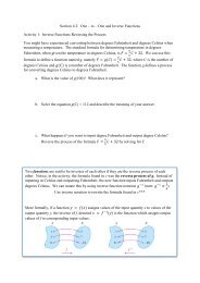
Figure 1.1 Location Map. The study area is located on the eastern shore of Summer Lake,
Oregon, in a field of sand dunes. The sand dunes have either formed or migrated into this
area in the last 8200 years, since pluvial Lake Chewaucan's most recent highstand. Desert
pavements and harvester anthills are found in the present dune field. Summer Lake only
occupies a small portion of pluvial Lake Chewaucan's former extent. The sand dune field
to the east of the lake overlies alluvium from the Chewaucan River, which currently flows
north into the town of Paisley, then turns towards the east.
2

Figure 1.2: Sand Dunes east of Summer Lake. These dunes have formed in an area
which was underwater 8200 years ago. The high concentration of sagebrush on the dunes
might lead to their classification as "semi-active" (Lancaster, 1995), but the area is under
constant eolian action, as evidenced by the dust storm visible between the dunes in the
foreground and winter ridge in the background (large clouds of dust often billow off of the
playa surrounding Summer Lake).
3

Figure 1.3: Desert pavement in the Summer Lake sand dunes. Desert pavements are
extremely common features in arid environments. A desert pavement is a surface deposit
of gravel-sized clasts (greater than two millimeters in diameter) overlying a fine-grained
soil. The uppermost horizon of this soil contains abundant vesicles formed by trapped air,
probably during rapid wet-dry cycling after rainstorms. In this photograph the pavement
has been compressed into the A horizon by vehicle traffic, causing the bright colored tire
tracks in an otherwise dark surface.
4

i n conj uncti on wi th a si l t- ri ch vesi cul ar "A" soi l hori zon ( Av) . Curr ent r esear ch holds
t hat bot h the deser t pavement and the Av hor izon requir e ari d cli mat ic condit ions and
l ong per iods of t im e i n whi ch t o f or m ( McFadden et al ., 1998). The Sum mer L ake sand
dunes appear to have experi enced m or e r apid deser t pavem ent for mati on than has
previ ously been r ecorded in t he scienti fi c lit er ature.
T he predom inant ant speci es i n the S umm er L ake sand dunes (t her e ar e at least
t wo smal ler twi g- mound buil di ng gener a) i s the Owyhee harvest er ( P ogonomyrmex
owyheei ) . The Owyhee har vester ant has the widest range of any Nort h Ameri can
har vest er ant , fr om nort her n Mexico in the south to nor t hern Br it ish Col umbia, and f r om
t he P aci fi c Ocean t o east er n Nor th Dakota, but i s among the least st udied ( Taber, 1998) .
I t is sm al ler t han som e of it s cousi ns (3mm rather than 6m m long) m aki ng it a l ess
att ract i ve r esear ch subj ect ( Gordon, 1999). Nonet heless, som e r esear ch has been done
on P . owyheei nest densit i es i n the I daho hi gh deser t ( Port er and Jor gensen, 1988).
Har vest er ant s buil d pebble-coat ed m ounds on t op of t hei r nests ( Fi gur e 1.4).
T here ar e sever al hypotheses to expl ain t he reason for thi s behavior , but t he acti on it self
has not been st udied, as bi ol ogi st s have been mor e concerned wi th i t s causes. An
hypot hesis curr entl y i n favor am ong ent om ol ogi st s i s that har vest er ants’ str ong sense of
smell l eads them to buil d t hese hi ll s usi ng rocks because por ous rocks hold t he colony’ s
scent , det er r ing ant s fr om ot her col oni es f r om vi si ti ng ( Gordon, 1999; Gordon, 1984).
A m or e classi c expl anati on is t hat t he pebbl es ar e a byproduct of subt er r anean
excavat i on of t he colony’ s home ( Br anner , 1910; F or el, 1929). I pr opose that t he ant s
are excavati ng these pebbles and pil i ng t hem i nt o ant hi l ls t o prevent the wind from
5

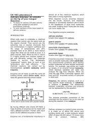
Figure 1.4: An Owyhee harvester anthill in the Summer Lake sand dunes.
Harvester ant colonies build gravel mounds over their homes, perhaps to protect the
colony from wind erosion, as they tend to live in arid environments. The colony may
live as long as twenty five years once the ants have established a gravel covered mound
(Taber, 1998). The cleared area surrounding the mound is also typical of harvester ants.
The gravels used in the construction of the anthill are usually less than five millimeters
in diameter, as illustrated by the ball-point pen in the above photograph, which is seven
millimeters in diameter.
6

erodi ng thei r hom es. I have al so at t em pt ed to i nvest igate t he mechani sm s by whi ch t hey
const ruct the ant hi l ls.
1. 2: Ai m s and Ob j e ct i ve s
T he pri m ar y obj ecti ve of this st udy was t o det er m ine whether harvest er ants have
hel ped devel op the deser t pavem ent i n t he S umm er Lake sand dunes. Thi s requi red t he
i nvesti gat ion of thr ee general probl ems. F i rst, I char act er i zed som e of the physi cal
propert i es of t he sand dune ecosystem , focusing on part i cl e size analysi s of the sand
dunes t hem sel ves, t he deser t pavem ent s that form in areas bet ween t he act ive dunes, and
t he all uvi um which under l ies the sand dunes.
S econdl y, I studi ed the rat e of anthi ll growth, the char acter isti cs of sedi ment s
i ncor por at ed into anthil l s, and the rel at ionship of other physi cal processes to ant
t ranspor t of sedi ments i n t he S umm er Lake sand dunes. The r ole of ant s as
biogeom orphi c agent s has been noted by ot her s ( Br anner , 1910; But l er , 1995) , but r ates
and processes by whi ch Owyhee harvest er ant s m odi fy t hei r physi cal envir onm ent have
not been f or m al ly i nvest i gated pri or to t hi s study.
T hi rdly, I sought t o expl ai n the r el ati onshi p bet ween t he pebbl es i n t he desert
pavem ent sur f aces and pebbl es i ncorporated int o ant hi ll s i n the study ar ea. Bot h
f eatures are composed of pebbles der i ved fr om al l uvium deposi ts t hat underl ie t he dune
f ield. Do harvester ant s par ti cipat e i n the f or m at ion of deser t pavem ent ?
7

1. 3: S t r u ct ur e of Thi s The si s
T he set t ing for t hi s i nvest igat i on i s descr i bed in chapt er t wo, whi ch pr ovi des a
gener al pi ct ure of the geol ogy and cl im at e of the study ar ea. The fol lowing si x chapters
each address a component of t he br oad quest i ons present ed above. T hese chapt er s each
i nclude the background i nform at i on and descr ipti on of t he met hods necessary f or thei r
r espect i ve t opi c.
I n chapt er t hree, I di scuss desert pavement s, bot h in t heory and in the Sum mer
L ake sand dunes. T his i s achieved t hrough det ai l ed study of sedi ments and of t he
f or mer locat i ons of pl uvi al L ake Chewaucan’ s shor el ines relat ive to deser t pavem ent
deposit s.
Because this thesis coul d not possibl y incor porat e detai led mappi ng of al l surf ace
deposit s f ound in t he dune fi el d, I att em pt to quanti fy these deposi ts, in part i cular t he
per cent age of t he ar ea m ant led wit h deser t pavem ent , thr ough remote sensi ng. Chapter
f our di scusses aeri al photogr aphic i nterpret at ion and r emote sensing t echni ques appl i ed
t owar ds this goal .
Har vest er ant s and ant hi l ls are the subject of chapters fi ve, six, and seven. I
present the resul ts of anthil l densi t y surveys i n chapt er fi ve and com par e my r esult s wit h
t hose of r esear cher s i n other ar eas. Chapt er si x i s focused on ant hil l const ructi on
m et hods and rat es. The field r esi n- i mpregnati on techni que I developed t o study anthi ll
str uctur e in detail is descri bed i n chapt er seven, al ong wit h m y fi ndi ngs.
My f inal quest ion, the rel at ionship between desert pavement , ant hi l ls, and
all uvium , is addr essed i n chapt er ei ght . T his chapter includes par t icle si ze anal ysi s of
8

t hese t hree disti nct t ypes of pebble- deposi t and st at ist ical compar i son of the thr ee
groups.
9

CH AP T E R 2: THE S UM ME R L AKE S AN D DUN E S IN CONT E X T :
MI OC E N E BAS AL T S , P L E I S T OCE NE L AKE S , AN D HO L OC E N E CL I MA T E
2. 1: Gene r a l Geo l o gi c S et t i n g
T he bedr ock in the Sum mer L ake basin consist s of late Mi ocene ( ca. 6-7 Ma)
t holeii t ic basalt s ( Di ggles et al. , 1990b; Jel li nek et al. , 1996) over lai n by Cenozoi c
t uf faceous sedi ment ary deposi ts. The basin fl oor i s cover ed wi th pl aya and all uvi al
sedim ent s. T he sedi m ents ar e mor e than 30 m thick at the nor t hern end of the pr esent
l ake ( Negr ini et al. , 2000) . Holocene sand dunes i n t he east er n par t of the basin ar e up
t o 10m thi ck ( Adri an et al ., 1993; Di ggl es et al. , 1990b) . The dunes over li e Chewaucan
River al luvi um of an unknown depth ( Di ggles et al. , 1990b). The Chewaucan Ri ver
f lowed nor th into t he Sum mer Lake basin unt i l the end of t he last gl acial per iod
( Al li son, 1982) . A sm all l ate Miocene / ear ly Pl iocene ci nder cone cal led Ten Mil e
Ridge outcrops in t he mi ddl e of the sand dunes ( F igur e 1.1; Diggl es et al ., 1990a) .
Nor th-sout h trending cli f fs of Miocene basal t cr eat e the east and west edges of the
val ley ( Tr auger , 1958) as i s typical of Basi n and Range topography i n the sout hwest er n
Uni ted States ( Br adley, 1982; S tewar t et al ., 1975) . The Brothers F aul t zone which cut s
t hr ough the nor theastern corner of t he vall ey is of ten ref er r ed t o as the nor thernmost
boundar y of the Basi n and Range physi ographi c pr ovi nce, whil e Winter Ridge to t he
west of Summ er Lake is consider ed to be i ts west ern boundary ( Di ggles et al. , 1990b;
Donat h, 1962; P hi ll i ps and Denburgh, 1971). The basin has under gone extensi ve
10

t ectoni c def orm at ion, wi t h the most recent maj or eart hquake (gr eater t han M 6.9)
occur ri ng at least 4000 years ago ( Langri dge et al. , 2001; Pezzopane and Weldon,
1993) .
S um mer Lake is in t he Basin and Range physi ogr aphic province ( Donath, 1962),
approxi m at el y 120 ki lomet er s east of Cr at er Lake, but pumi ce fr om Mt . Mazam a’ s 6845
years BP erupti on i s f ound near the present - day shoreli ne ( Al li son, 1945; Davi s, 1985).
S om e researcher s have al so descr ibed the Sum mer Lake sand dunes as bei ng excl usi vely
com posed of Mazam a ash and pumi ce ( Negr ini , 2001) . The Sum mer L ake area is
wit hi n the heavy bl ast zone ( deposit s > 15 cm thi ck; Wil li ams and Goles, 1968) fr om
t he cli m at ic er upti on of 6845 +/ - 50 year s BP ( Bacon, 1983) .
2. 2 Cl i m a t e at S um m er L ake
P resent - day Sum mer Lake is a rem nant of pluvial Lake Chewaucan (F igure 2. 1) ,
one of the nort hernm ost of the ice-age Basi n and Range lakes ( Fr iedel , 1993) . Lake
Bonnevi l le, of which t he Gr eat Sal t Lake is the present remnant , was t he fi rst of these
f or merl y m assive lakes t o be ident if i ed by Russel l on hi s 19t h cent ury r econnai ssance
geology expedit ions to t he west ern U. S. ( Russel l , 1885) . Pl uvi al l akes for m in cl osed
basins in the wester n Uni ted St ates dur ing ice ages when t he pr esence of a large i ce
sheet t o t he nort h for ces t he sub- pol ar j et st ream sout h of its i nt erglacial posit ion
bri nging m or e preci pit at i on t o present day deser t s ( COHMAP , 1988; Wendl and, 1989).
At Summ er Lake, appr oxim ately 1300 m above sea l evel, t he Pl eistocene was
r ai ni er than the pr esent , and t he al pine snowl ine m ay have been as much as 800 m l ower
t han it is now (Wigand, 2001) . The trees t hat curr entl y occur only on r i dges above
11

Summer
Lake
Chewaucan
River
Ten
Mile
Ridge
Shoreline of
Pluvial Lake
Chewaucan
Figure 2.1: Pluvial Lake Chewaucan. The present-day Summer Lake sand dunes are
located to the east of the lake in the area occupied by the lake at its maximum recorded
extent 30,000 years ago (Allison, 1982).
12

S um mer Lake wer e pr obabl y f ound at l ower el evati ons near i ts shor el i nes dur ing
t he P lei st ocene. T he speci es r epr esent ed i n pol l en f rom l ake sedim ent cores wer e the
sam e as those f ound pr esent ly, but r elati ve abundances wer e dif ferent (Cohen et al .,
2001) .
P luvi al Lake Chewaucan covered the curr ent locat i on of the sand dunes dur ing the
P leistocene ( Al li son, 1982; Reheis, 1999) . The pluvi al lake has been ext ensi vel y
docum ent ed because its sedi ment s r ecord t he last paleom agnet i c rever sal ( Davi s, 1985;
Negri ni and Davis, 1992; Negr ini et al. , 1988) . Twel ve thousand years ago pl uvi al Lake
Chewaucan occupied bot h the S um m er and Aber t L ake basins. Appr oxim ately 8000
years ago the l ake receded, l eaving behind two separate lakes. All i son ( 1954) identi f ied
sever al terr aces at el evati ons bet ween 1277 and 1377 met er s (4190 and 4520 feet ) above
sea l evel. The m odern el evat ion of the l ake i s about 1264 m eters ( 4150 feet) . Al li son
( 1982) later cor rel at ed t he 1377 meter ( 4520 foot ) elevat ion shorel ine wi t h a radiocar bon
age of 30, 700 years B. P . He i denti f ies the 1357 m et er (4455 f oot) shor eli ne wi th a
17, 500 years B. P . radiocar bon age, and t he 1337 meter (4385 foot ) ter race as t he most
r ecent impor t ant shoreli ne, car ved duri ng t he mi nor pluvial epi sode which ended
approxi m at el y 8000 years ago (F i gure 2. 2) . The presence of thi s shoreli ne is
unexpect ed ( L icci ar di, 2001) . Duri ng the 8200 yr BP cold event the m aj ori ty of pluvial
l akes i n t he Gr eat Basin were not rej uvenat ed ( Benson et al ., 1990), but L ake
Chewaucan ref il led its basi n ( Fr iedel , 1993; Negr ini, 2001) connect ing the present day
S um mer and Aber t lakes.
13

modern
historic
17,500 ybp
30,000 ybp
10 0 10 20 Kilometers
W
Figure 2.2: Former and current extents of Summer Lake and Lake Chewaucan. �
The largest lake shape shown in this image represents the 30,000 year pluvial shoreline, �
the next largest is the 17,500 year shoreline, and the two small lakes on the left are modern �
Summer Lake and the historic extent of Summer Lake recorded during the Fremont party's �
visit to Oregon in the 1840s.
N
S
E
13

T here i s an abundance of desert varni sh on pavem ent s and out crops i n t he sand
dunes t hat demonstr ates the ari dit y of this ar ea. The closest meteorologic stat ions ar e
l ocat ed in t he towns of Pai sl ey, t o the sout h and S um mer L ake, to t he nor thwest of t he
l ake (F i gure 1. 1) . Accor di ng t o Kienzl e ( 1999) the eastern edges of si m il ar basi ns wi th
ari di c soi ls in t he sout her n por ti on of L ake County r eceive an aver age r ainfall of 0. 2 m
per year , mostl y in the for m of summ er thunder st orm s. The t emper at ure r egi me f or
such soi ls i s m esic: aver aging 0.6 ˚ C wit h a f rost- fr ee peri od of between 70 and 110
days. At P ai sley the Oregon Cli m at e Ser vi ce recor ds a m ean annual ai r tem peratur e of
8.9 ˚ C, and at Summ er Lake they recor d a mean annual ai r t em per at ur e of 7.5 ˚ C. Bot h
of these t owns ar e locat ed in f ar mor e hospi tabl e cli mat es t han t he sand dunes on the
eastern shor e of the l ake. T he dunes are very spar sely veget at ed wi th sagebr ush and
occasional gr asses. T her e is a large popul ati on of har vester ant s, as well as other desert
ani mals such as j ackrabbi ts and li zar ds.
2. 3: S i t e Char ac t e r i z at i on : Th e S um m er L ak e Dun e F i e l d
T en Mil e Ridge is a pr om i nent geographi c feature fr equentl y ref er red t o in this
t hesi s. S and dunes form a semi - cont i nuous sheet through m ost of the f iel d ar ea, as wel l
as occur ri ng in i ndi vi dual cr escents on T en Mi le Ri dge. L ake Chewaucan’ s m ost recent
pluvi al maxi m um covered the areas that now com pr i se t he dune sheet (Pl at e 1), but the
r idge pr oj ect ed out of t he water . Desert pavements on Ten Mi le Ridge ar e com posed of
coarse (10-30cm ), heavil y var ni shed basal ti c cinder clasts wi th wel l -developed soi ls.
T hey ar e sim i lar to the classic deser t pavem ents descri bed by Wel ls et al . ( 1985) in t he
southwestern U. S. T he evi dence for extensive soi l -devel opm ent com bi ned wi th t he
15

l engt h of ti m e that these r esear cher s prescr ibe for sim i lar deser t pavem ent developm ent
i ndicat e t hat t hi s area is di st i nctl y dif fer ent than lower el evat ions whi ch wer e underwat er
8200 years ago (Chapter 3).
Deser t pavem ent s at el evati ons bel ow 1337 m eters (4385 feet) ar e com posed of
wel l- rounded pebbles der i ved fr om the all uvi um underl yi ng the sand dunes. The soi l
profi les beneat h these desert pavements are di st i nctl y dif fer ent fr om those on Ten Mi le
Ridge, wit h vesicul ar A hor izon devel opment , but li tt le to no other soil hori zonat ion.
All uvium f rom t he Chewaucan River was sam pl ed at a vari ety of l ocat i ons around
t he sand dunes (P lat e 1) , but was not r eached dur ing cor ing of the dunes (discussed in
Chapt er 3) . It i s ver y poorl y sor ted, wi th part i cl es r anging f rom clay (less t han t wo
m icrons) t o cobbl e (6- 26 cent im eter) si ze ( Bl ai r and McPher son, 1999) . These sam ples
wil l be di scussed i n greater depth i n Chapt er 8.
T he dune sheet is composed of f i ne sand, for whi ch ther e are two li kel y sources.
P ar ti cl e size of the sand var ies onl y sli ght ly t hroughout the study ar ea (F igur es 3. 7 and
3.8). The esti mated 15 cm of Mazama ash and pum i ce whi ch bl anket ed the val ley 6800
years ago ( Wi ll iam s and Gol es, 1968) coul d have been rewor ked i nt o dunes but cannot
account for a t en m eter thi ck dune sheet. Def lat ion of the Sum mer Lake playa over t he
l ast 6000 years m ust also be an im por tant sour ce of dune sand. T he pl aya sedim ent s in
t he val l ey ar e pr edomi nantl y si l t and clay sized (F igur e 2.3) . Dessicat i on cracks i n t hese
playas all ow the wi nd to easi ly er ode t hi s sedim ent ( Bagnol d, 1954; Glenni e, 1970;
Mabbutt , 1977).
16

Weight Percent
30
25
20
15
10
5
0
10000
1000
Figure 2.3: Particle Size of Playa Sediments. These three samples from playas in
the study area (see Plate 1 for locations) demonstrate that the dominant particle sizes
in playa sediments are silt and clay.
100
Particle Size (microns)
10
SD6playa
SD7playa
DP3playa
17
1

CH AP T E R 3: DE S E R T PAV E M E NT
3. 1: I nt r od uct i o n to De ser t Pa vem en t
T he classi c image of t he desert which m any peopl e have gai ned f rom movies such
as “L awr ence of Arabia” is an endl ess sea of sand dunes. Thi s is not a reali st i c
def init i on of a desert , as most deser ts i n the worl d ar e covered wi t h rocks or crust y soi ls
( Abraham s and P ar sons, 1994; Cooke et al. , 1993; Mabbut t , 1977) . Such deser ts oft en
exhibit a sur face l ayer of rocks one to t wo cl ast s thick above a soi l or ot her fine grained
deposit , r ef err ed t o as deser t pavem ent by Ameri can geom or phologi st s ( Gi lber t , 1875;
Mabbutt , 1977). El sewhere, t hi s sur face deposit i s cal led a gi bber pl ai n or st ony m ant le
( Aust ral ia), hamm ada, reg, or seri r (Ar abic) , or gobi ( centr al Asia) . Br it ish
geomorphol ogi st s usual ly adopt the name used i n the countr y of st udy, as such surf aces
do not exi st in t he Br it i sh I sl es.
A t extbook desert pavement (F igure 3. 1) i s a sur f ace coati ng of clasts i n whi ch
approxi m at el y 70 per cent of t he cl ast s ar e par ti all y em bedded i n the underl yi ng soil ,
wit h 20 percent of the surf ace of each cl ast embedded ( Cooke, 1970) . The clast s
protr ude i nt o a sil t y fi ne- gr ai ned "A" soil hori zon appr oxim ately 15 cm thi ck, contai ni ng
small vesi cl es or ai r bubbl es. Below t hi s is a B hor izon, between 20 and 60 cm in
t hi ckness, wi th an average (f or pavem ent mantl ed soil s in Cal if or ni a and Chil e) cl ay
content of ar ound t en per cent , whi ch is also f ree of coarse par ti cl es. The C hori zons of
soi ls beneat h deser t pavement s tend to be r i cher in coar se part icles t han t he A and B
18

Figure 3.1: Classic Desert Pavement in the Summer Lake sand dunes. This is an
area of fine (0.5-5 cm clast size) desert pavement located near Ten Mile Ridge (the
cinder cone visible in the background). The scattered sagebrush visible in this photograph
are surrounded by small piles of sand. Desert pavement is a surface deposit of
gravel which overlies a fine grained soil without any gravel in it. Desert pavement is
a common feature of deserts, but its origin is hard to determine.
19

hor izons above them . They usual ly over li e eit her all uvi um or bedrock, which ar e t he
t wo m ost com m on sour ces of coar se par ti cl es for pavem ent s ( Cooke, 1970; Dixon,
1994) .
T he vesi cular A hor i zon (Fi gure 3. 2) is a f eat ur e pecul i ar t o deser t soi l s
( Bi rkel and, 1999; Di xon, 1994; Dunker ley and Brown, 1997). It s disti nct ive textur e is
devel oped when ai r or ot her gasses ar e tr apped wi thin t he soi l duri ng som e type of
m or phol ogi cal change. I t has been cr eated in labor at or y envi ronm ent s by repeat edl y
wet ti ng and drying a beaker f ul l of soi l ( Bunt ing, 1977; E venar i et al ., 1974; S pr inger ,
1958) . Vesi cle developm ent m i ght not r equir e deser t pavem ent clasts at the surf ace of
t he soi l , but i t does requi re some sort of sur face seal i ng ( Dunker l ey and Br own, 1997) .
T here i s consider abl e debat e as to whet her microorganism s ar e i nvol ved i n t hi s process
( Kr um bei n and Giele, 1979; McFadden et al ., 1998) . Ther e i s also a gener al st at e of
confusi on about t he st abi li ty of vesi cular A hor i zons i n wet - dr y cycles succeedi ng t hose
whi ch m ay have form ed them. Thi s hor izon i s com m only r eferr ed to as t he "Av"
hor izon, alt hough t his i s not an off i ci al t axonom ic t er m ( Soil S urvey St af f, 1999) .
3. 2: How Do es De se r t Pa vem en t For m ?
T he f undam ent al problem under lyi ng m odern desert pavement st udi es i s
det er mi ning how clasts ar e concent rat ed on the surf ace. Many physi cal pr ocess
hypot heses have been i nvoked to expl ain desert pavement s. T hese include defl at i on
( Gi lber t , 1875; Hooke, 1966; Mabbutt , 1977; Shlem on, 1978) , sheet f lood ( Wi ll iam s and
Z im bl em an, 1994), erosi on of fi nes dur ing r ai nf all events ( Wainwr i ght et al ., 1995) ,
deposit i on of f ines beneath t he cl ast sur face thr ough eoli an forcing
20

Desert Pavement
Cleared Surface
7mm diameter pen
vesicle
Figure 3.2: Vesicular A horizon in the Summer Lake sand dunes. Vesicular A horizons,
commonly referred to as "Av" horizons, are found beneath desert pavements and other
soil crusts in arid environments. They have been experimentally created through
repeated wet-dry cycles in laboratories. The vesicles in this Av horizon, which occurred
beneath a "fine" desert pavement south of Ten Mile Ridge, are near in size to the pavement
clasts (between one and five milimeters in diameter). The pebbles which formed
the pavement can be seen at the left side of the picture.
21

( McFadden et al ., 1998; Wel ls et al. , 1990) , chemi cal di ssol ut i on of all cl asts in t he soil
save those at t he surf ace ( Goudie and Par ker, 1998) , and f r eeze- thaw cycl ing ( Ingl is,
1965; Matsuoka, 1995). Regar dl ess of for mati on mechani sm , t hese st udi es have all
r epor ted t hat deser t pavement s are st able surf ace coati ngs f or fi ne- gr ai ned sedi ment s or
soi ls.
Of the many processes pr oposed for desert pavement form ati on, onl y def lat ion can
be physi call y appli ed in al l envir onm ents wher e deser t pavem ent s ar e f ound. The
def lati on model assumes an init i al ly very t hick soi l or unconsoli dat ed sedi ment ary unit
containi ng a sm al l propor ti on of gravel -sized cl ast s. Over tim e, t he soi l er odes away,
l eavi ng the gravel as a lag deposi t at the sur face ( Gi lber t , 1875) . If t he soi l below t he
pavem ent i s representati ve of t he ini ti al coar se- part icl e concent rat ion above t he pr esent
ground sur face, est i mates of the i ni t ial thi ckness of soil r equir ed to cr eate t he exi st ing
stony surf ace l ayer s woul d requi re t he form er pr esence of physi call y unr eal isti c amount s
of soil in m any envi ronm ent s ( Cooke et al . , 1993; Mabbut t, 1977). This has led
r esearcher s to speculate on a number of sit e-specif ic m odels to expl ai n deser t pavem ent
f or mati on.
T he m ost popular model at present is that of Wel l s and McF adden, in which clast s
are slowly separated f rom an exposed bedr ock sur f ace by the incor por at ion of eol ian
dust int o cr acks in the rock ( McFadden et al ., 1987; Wel ls et al. , 1985) . This pr ocess
r equi res t ens of thousands of year s and i s most appli cable t o per fectl y flat bedrock
sur faces such as lava fl ows. I t i s not wel l sui t ed t o abandoned al l uvial f ans, on which
deser t pavem ent s ar e oft en found ( Hooke, 1990) . This model also rai ses t he
22

f undamental quest ion of whether the def init i on of deser t pavement r equir es an
under lyi ng f i ne-grai ned soi l.
Quade ( 2001) suggest s that deser t pavem ent is not as st abl e as pr evi ous studi es
have dem onst r at ed, and questi ons i ts pr eser vat ion t hr ough gl aci al peri ods. His work in
t he Deat h Val ley region of Cali f or ni a and Nevada found that no deser t pavem ent older
t han the l ast glaci al (12.5ka) is pr eserved above 400m elevat ion. He does not ident i fy
l ocal pl uvial l ake sur face el evati on. He al so bases these dates on deser t varni sh, whi ch
m ay be a f aul ty m et hodol ogy f or dati ng surf aces. ( Br oecker and L iu, 2001)
Recent wor k suggest s t hat biota of m any sizes (f r om beet les to burr os) m ay pl ay a
r ol e in the inf lati on pr ocess descri bed above by rocking clasts back and fort h to al l ow
f ines t o be emplaced beneat h them ( Haff and Wer ner, 1996). The wor k discussed in this
t hesi s suggests yet anot her possibil i ty, in which biologic agents ( har vester ant s) excavate
t he clasts and pl ace t hem on top of the f ine-grai ned sand dunes.
3. 3: Dese r t Pa ve m e nt s Obse r v ed at S um m er L ake
T wo dif f er ent styles of deser t pavem ent are pr esent i n the st udy ar ea (F i gure 3. 3) .
T he f ir st type is f ound on the sand dunes and is composed of sm al l (2m m- 1cm ), well -
r ounded pebbl es of var ious li thologi es, der i ved from al l uvium under l yi ng the sand
dunes i n t hi s area ( Di ggles et al. , 1990b). Deser t pavem ents on T en Mi le Ri dge, above
t he 8200 year s B. P . highst and of Sum mer Lake, consist of lar ge ( centi met er s wi de)
f latt ened heavi ly varnished basalt ic ci nder cl ast s.
T he A hori zons of soil s beneath these t wo t ypes of pavem ents shar e sever al
charact eri st i cs. Both have wel l -developed vesicular textures. T hi s i s to be expect ed as
23

Figure 3.3: Two types of desert pavement exist in the Summer Lake sand dunes. The upper
photograph is from Ten Mile Ridge, above the 8200 year B. P. shoreline of Lake Chewaucan. It
shows a coarse-grained desert pavement composed of bedrock fragments. The lower photograph
is of fine desert pavement with clasts derived from the alluvium that underlies the sand dunes.
The 7mm diameter pen in the lower photograph is wider than most of the pebbles in this pavement,
the hiking boot in the upper photo is similar in diameter to the pavement clasts there. 24

ot h have exper ienced the sam e cli mat ic condit ions duri ng the l ast 8000 years. They
share si mi lar soi l par ti cle sizes (m ode of 200 m i cr ons) , and extr em ely basi c pHs
averagi ng about 10.2 (AST M 1:1 di st il l ed wat er met hod) . A hi gh pH i s t ypi cal of deser t
soi ls wher e the ari d cli m at e resul ts in a l ow or ganic m att er cont ent ( Cooke et al . , 1993) .
All of the soil sam ples col lect ed in the st udy ar ea eff ervesce vi ol ent ly when weak
hydrochl or ic acid i s appl ied to them , i ndicati ng a hi gh calci um car bonat e content. Thi s
i s typi cal of deser t soi l s, as there is l it t le r ainfall to wash car bonat es away, and the low
organic matt er cont ent l i mi ts di ssol uti on by organi c aci ds ( Dunker l ey and Br own, 1997) .
Bel ow t he A hor izon, soi l s under lying t he t wo types of pavem ent are di st i nct.
F ine- gr ained pavements f ound in the dune fi eld over li e imm at ure A-over -C soil s. S oi l s
beneath the coarse- grained pavem ents on T en Mi le Ri dge are m ore developed, wi th
r eddened B hori zons. The t hi ckness of the soi l beneath the fine- gr ained pavements i s
dif fi cul t to determ i ne because the C hori zon blends i nt o t he underl ying dune sand. The
soi l beneath coar se- gr ai ned pavement s i s thi n; weat hered bedr ock occur s at a depth of
approxi m at el y 50 cm .
T he sedi ment s beneat h the f ine- grained deser t pavem ents have a hi gh CaCO3
content which has part ial ly cem ent ed the soi l. A t ypical st r at igraphy i ncl udes a 6- 10
m m thick l ayer of f i ne pebbles and coar se sand, overl yi ng a 10 cm t hick layer wi th
ext remel y dense vesi cl e concent r at ions, a 20cm t hick layer wi th i nt erm it t ent vesicles,
and upwards of 60cm of f i ne sand wit h ver y int er m it tent coar se sand / fi ne pebbl e si zed
par ti cl es pr esent i n i t (Fi gure 3. 4) . This can be cont r asted wit h all uvi um f rom l ocati ons
25

Desert Pavement
Alluvial Cobble
Vesicular A horizon
Non-vesicular silty horizon
Cleared Surface
Foreground Soil Surface
Weathered soil horizon in alluvium
30 cm
shovel
blade
Figure 3.4: Desert Pavement Stratigraphy. The stratigraphy beneath a fine-grained
desert pavement in the Summer Lake sand dunes (Site DP7 on Plate 1). One to two
centimeters of loosely packed pebbles overlie a ten to 15 cm thick vesicular A horizon,
which in this location lies over a dense silty horizon without vesicles and a weathered
soil horizon in poorly sorted alluvium from the Chewaucan River. In other parts of
the study area there may be two to three meters of dense sand between the surface and
alluvium.
26

around the dune sheet, which contains a wide r ange of part icl e si zes, fr om cl ay to 10cm
cobbl es.
3. 4: F or m a t i o n of De se r t Pa ve m en t s at S um m er L ake
T he t wo types of deser t pavem ent i n the study ar ea appear to have been cr eated by
dif ferent pr ocesses. They ar e sim il ar in m any char acter isti cs, but the dif ference i n soi l
devel opm ent suggest s t hat t he coar se- gr ai ned desert pavement s are ol der than the f ine-
grained deser t pavem ents. The lar ge part icl e si ze deser t pavem ent on Ten Mil e Ridge
probabl y f or m ed t hr ough inf lati on ( McFadden et al ., 1987; Wel ls et al. , 1985) . This
t ype of pavem ent is only found above 1341 m eters (4400 feet) in elevat ion. T he Ten
Mil e Ri dge pl at eau has been subaer ial ly exposed since pl uvial L ake Chewaucan’ s
P leistocene highstand, 17,500 r adi ocarbon year s B.P . ( Al li son, 1954; F igur e 3.5) . T he
m ost recent pluvi al maxi m um of 8200 years ago cor responded wi th a shor el i ne at
1337m el evat i on ( Fr iedel , 1993; L icciardi , 2001) .
F ine- gr ained desert pavem ents exist at el evati ons bel ow the most recent pluvi al
highstand. They exhibit cl assi c desert pavement st rati graphy, and in fact have thicker
f ine gr ained deposi t s beneath t hem t han t hose on Ten Mi l e Ri dge. I f bot h pavem ent s
f or med thr ough infl ati on, t hese fi ne- gr ai ned pavement s would have t o be older t han t he
coarse- grained pavem ents which have thi nner soil s under l yi ng them . The pluvi al
history and the soi l developm ent dif f er ences bot h suggest an ol der age f or the coarse-
grained deser t pavem ents. This means t hat the f i ne-grai ned deser t pavem ent s must have
f or med thr ough some pr ocess other than infl ati on.
27

W
N
S
E
"∂ 'a
*a
*b
" b
1 0 1 2 Kilometers
Figure 3.5: Locations of Desert Pavement in the Study Area. The islands in the
upper middle portion of this image are peaks on Ten Mile Ridge (Plate 1). The light blue
colored area in this image (clipped from a map of the extents of pluvial Lake Chewaucan,
prepared using ArcView GIS software) represents the 8200 year b. p. shoreline of pluvial
Lake Chewaucan. The darker blue is the 30,000 year shoreline (elevations from Allison,
1982). Point "a" is the GPS location of the coarse-grained desert pavement shown in
Figure 3.3, while point "b" is the location of the fine-grained pavement shown in the same
figure.
28

3. 5: Met h od s: Se di m en t s in t he Su m m er La ke Sa nd Du ne s
S edim ent cor es were hand- augered at thr ee si tes in the study ar ea ( F igur e 3.6,
P late 1) . T he dept h r eached at the “SD” si t e was 3.2 m eters beneat h t he surf ace of that
l ar ge acti ve dune. This si te i s l ocated in the center of the study ar ea, ami d lar ge roll ing
sand dunes wi th i nt erm it t ent pat ches of f ine desert pavement and sm all pl ayas. The
other borehol es att ained dept hs of sl ight ly over a meter . One of t hese is at t he "painted
hil ls" sit e at the southern end of t he dune sheet , whil e t he ot her is on a large crescent ic
sand dune on Ten Mi l e Ri dge. T he locat ions were determ i ned usi ng a Tr im ble GPS
uni t.
S am pl es were coll ect ed f r om t he auger r oughl y every 10 cm depth at each sit e.
T he sam ples wer e caught in zi pl ock bags and numbered wi t h the sit e nam e and t he
depth. Sampl ing depth was deter mi ned by runni ng a st eel m easur ing tape to the bot tom
of the hol e aft er t he auger was removed. Detail ed anal ysi s was per f or med on the S D
and P H sam pl es. The T en Mi le Ri dge sam pl es were char act er ized using f iel d
obser vat ions.
T he sam ples wer e ai r -dri ed in t he lab pri or to part icle si ze anal ysi s. Each sam pl e
was wei ghed, then wet si eved thr ough a #230 si eve i nt o a 1000 m l set tl ing col um n usi ng
disti ll ed wat er . T he coarse fr act ion was t hen dr ied in an oven at around 105 degr ees
Cel ci us befor e re-weighi ng. I det er m ined t he par ti cl e size fract ions for t he l arger than
63 mi cr on por ti on of each sam pl e usi ng a st ack of U.S . Standard S ieves and a W. S.
T yl er Corpor ati on RX-86 Sieve S haker . Each sampl e was mechanical ly si eved for 15
29

Figure 3.6: Augering at the "SD" site in the Summer Lake sand dunes. Using the
auger (held by field assistants Meghan Lunney and Jennifer Edmundson) shown in
this photograph we extracted samples every ten centimeters to a depth of 3.2 meters.
The auger becomes unsteady with the addition of the fourth and fifth stem-segments.
30

20 mi nut es ( McCave and Syvit ski , 1991; McManus, 1988). The sil t and clay size m ass
f ract ions wer e deter mi ned usi ng the pipet te method ( Syvi tski et al ., 1991).
3. 6: Res ul t s: S ed i m e nt s i n th e S um m er L ak e S an d Dun es
T he par t icle si ze pr of il e beneat h the "SD" sit e includes f our bur ied desert
pavem ent hor i zons ( F igur e 3.7). T hese hori zons are separated by pebbl e- f ree sand.
Bur ied pavem ent s ar e i denti fi ed based on the absence of pebbl es i n the samples above
and bel ow them in t he cor e. Each cor e sampl e captures a r oughl y 10cm int er val. T he
bur ied pavem ent sam ples include a subst anti al num ber of part i cl es gr eater t han 2mm i n
diameter . Augeri ng ended at 3. 2 m dept h when we encount er ed a large r ock i n ei t her a
pavem ent hor i zon or the all uvium beneat h the dune sheet (Appendix A) .
T he cor e at the pai nted hil ls si te ( F igur e 3.8) in the southern dunes of f er s an
i nt ri gui ng pi ct ur e of the Mazam a ash. The upper 0. 6 m of thi s core cont ains pebbl e-
sized pumi ce cl asts that ar e not present lower i n t he core, and whi ch may have been
concent r at ed by bul k densit y rel at ed er rors in sample spli tt i ng, bot h in the fi eld and in
t he l aborator y. Bel ow 60 cm the coar se par t icles are al luvi al pebbl es si mi lar to those
f rom deser t pavem ent s in the ar ea. We st opped cori ng at 1.3m due t o cont act wi t h a
dense l ayer of pl aya or cal cr et e sedi ment s (Appendi x B) .
T he sand dune cor ed at T en Mi le Ri dge was unif or m ly f ine-grai ned. There were
no pebbl es pr esent unt il we r eached bedrock or coar se desert pavement at 1. 5 met er s
depth.
31

0 m depth
buried pavement horizon, 2.2m
buried pavement horizon, 2.5m
buried pavement horizon, 3m
buried pavement horizon, 3.2m
3.3m depth
particle size (microns) diminishing to the right
Figure 3.7: Particle Size profile from "SD" site. The squiggly lines in this figure are
particle size frequency curves (weight percent on the y-axis, particle size on the x-axis)
placed according to approximate depth.
32

particle size (microns) decreasing to the right
0 m depth
1.2 m depth
Figure 3.8: Particle Size profile from "PH" site. The squiggly lines in this figure are
particle size frequency curves (weight percent on the y-axis, particle size on the x-axis)
placed according to approximate depth. The maximum depth reached in augering at this
site was 120 cm. The upper portion of the core contained abundant pumice clasts, visible
in the left-ward leaning of the peaks at the top of this figure.
33

3. 7: Di s cu ssi on
T here ar e two disti nct desert pavement types i n the S um m er L ake sand dunes.
P avem ent s on Ten Mi l e Ri dge above the m ost recent pluvi al shoreli ne ar e com posed of
coarser cl ast s and contai n fr agm ents which have been det ached f rom local bedr ock
sur faces t hr ough an infl ati on pr ocess l ike that descr ibed by Well s et al . ( 1985) .
P avem ent s bel ow t he 8200 year B. P . shoreli ne ar e com posed of f ine (usual ly l ess t han
one cm in di ameter) pebbl es der i ved from al l uvium . T he al luvium is at a far gr eat er
depth below the sur f ace of the sand dunes t han t he bedr ock on T en Mi le Ri dge is below
t he desert pavement s f ound ther e. Both t ypes of pavement exhibit vesi cul ar A hori zons
and clast- fr ee lower soi l hor izons. The “f i ne-gr ai ned” deser t pavem ents must evol ve
t hr ough a di f ferent and previ ously unexpl ai ned m ethod. They ar e geogr aphical ly near
t he coar se pavement s, exhibit t hicker t hough l ess m at ur e soi l hor izons, and have
evolved in l ess t han hal f t he t i me avai labl e f or the for mati on of t he coarse pavem ent s.
T he dunes ar e com posed of f ine sand (mode of 200 mi cr ons). There have been at
l east f our peri ods of deser t pavem ent f or mat ion, as evi denced by the f our bur ied
pavem ent hor i zons encount er ed at t he SD sit e. Carbon dati ng of t he pavem ents woul d
l ikel y yield unhelpf ul r esult s. Organi c mat ter in the dunes is l ar gel y der ived fr om sage
brush, whi ch has roots t hat coul d easil y reach t he dept hs of the bur ied pavem ent s
( Di ggles et al. , 1990b). The area is al so home to ant s, whi ch are fr equentl y blamed wit h
disrupt i ng sedi ment s f or soil -f r acti on carbon dat ing pur poses ( Hedges and Gowlett ,
1986; S charpenseel, 1979) .
34

Another potenti al m ethod of dat i ng desert pavements t hat was reject ed for use i n
t hi s st udy i s t o dat e deser t var ni sh found on them. Deser t var ni sh is a bact er i al buil dup
f ound on t he surf ace of rocks i n ari d envir onm ent s (Dor n and Ober lander, 1981). T hi s
m et hod has been standardi zed thr ough fr equent use ( Dorn, 1986; Fr iedel , 1993;
Har ri ngt on and Whit ney, 1987; Quade, 2001). Recent wor k by Liu and Br oecker ( 2000)
poi nt s out t hat desert varnish does not grow at uni form rates, even in di ff er ent l ocati ons
on the sam e piece of r ock, maki ng it unreli abl e for dat i ng. The sam e aut hors ( Br oecker
and L iu, 2001) al so demonst rated that deser t var ni sh does not necessar il y recor d
t em perat ur e, only a lack of r ai nfall .
Mazam a ash i s present at the souther n end of t he dune sheet, as i ndi cated by
pebbl e sized pumi ce fr agm ents f ound in the sedim ent s and at Five Mi l e Cave ( Al li son,
1945) . The Mazam a sedim ent s found at t he "pai nt ed hi l ls" si t e ar e coarser than those
f ound i n eit her t he al luvium under lyi ng t hem or the l ar ge sand dunes at the "SD" sit e.
T he pebble si zed pum ice fragm ent s ar e absent i n the sedi ment s auger ed out of the "SD"
sand dune, and they ar e also absent in near by deser t pavem ent sam pl es. Whi le m y
sam pl ing suggests t hat Mazama deposi t s ar e absent f rom much of the study ar ea,
det ai led chem ical anal ysi s of sedi ments f rom a vari et y of locat ions in t he dunef ield is
necessar y to rule out the possi bil it y t hat the dunes ar e com posed of r eworked Mazama
deposit s.
35

CH AP T E R 4: AE R I A L PHO T O GRA P H I C ID E N T I F I C AT I ON OF DE S E R T
P A VE ME NT CO NCE NT RA T I O N
4. 1 Re m ot e Sen si ng Mo t i vat i o n
I n this chapt er I di scuss t he m ethods used to est im at e the percentage of the st udy
area cover ed in desert pavement . Quant if icati on of t he im pact of harvest er ant s on the
f or mati on of desert pavem ent i n t he Summ er Lake sand dunes requi res an est im at e of
t he area covered by pavem ent. Tradi t ional mappi ng is t oo ti m e and labor intensi ve t o be
a pract i cal met hod. Aer i al phot ographi c int er pr etati on has been pr oposed as an ef fi cient
and cost -eff ect ive alt er nat ive to fi eld m apping, and it s usef ul ness is eval uated her e.
Researcher s oft en use di f ferences in spectr al charact er i st ics t o di f ferenti at e ari d
l and- sur face feat ur es. For exam pl e, Ri vard et al . (1992) used spect ral val ues to cl assif y
sand dunes and varni shed rocks in the Middl e E ast . T hat and ot her studi es have used
L andsat TM and MS S, SP OT , and ot her sat el li t e rem ot e sensi ng data t o classi fy l and
sur face types ( Bull ar d et al. , 1995; E l -S heikh and Syiam, 1989; Jacobber ger et al . , 1983;
S hi pm an and Adams, 1987; Weit z and F arr , 1992; Z i mbel man and Wi ll iam s, 1996).
Whi le aeri al phot ogr aphs coll ect onl y one band of panchr om at i c li ght , it is expect ed that
som e analogy can be dr awn t o ear li er anal yses of rock and sedim ent albedos (F igure
4.1). Aer ial photographs wer e used her e because avai lable satell it e coverage i s eit her
prohi bi t ivel y expensive or of l ower resol ut i on t han avai labl e aer ial phot ographs.
36

Figure 4.1: Surficial deposits in the Summer Lake sand dunes. Desert pavements (in
the foreground with the tire tracks) are darker and less reflective than sand dunes (present
in the background of this photograph). It should be possible to differentiate between the
two based solely on this observation about their spectral characteristics.
37

4. 2 Ae r i a l Pho t o gr aph s
T he onl y avai labl e photographs cover i ng t he east ern side of Sum mer Lake are
black and whi te pri nts f r om t he Nati onal Aer ial Photogr aphy Progr am (NAP P ) (USGS
E ROS web page,
htt p: // edc.usgs.gov/ Webgl is/gli sbi n/ f inder_m ai n. pl?dataset _name=NAP P rechecked 2-
27- 2002; E d Zigoy of t he BL M Por tl and off ice, per sonal com municat ion, 11- 98). The
NAP P photogr aphs have a maxim um resol ut ion of 1: 40, 000, lower t han the 1: 10,000
r esol ut i on t hat woul d have been ideal .
Deser t pavem ent can be di st ingui shed at t he 1: 40, 000 resol ut i on ( Bull ar d et al. ,
1995; L aymon et al. , 1998) . However , it is not rel iabl y disti nguishable f r om bedr ock
wit hout the inclusi on of ul tr avi ol et or i nf r ar ed radi at i on ( Weit z and F arr , 1992) . An
i ni ti al objecti ve was to di st ingui sh between t he fi ne and coarse deser t pavem ent s
descr ibed in chapter t hr ee, and to i denti fy the presence of veget at i on or soi l crust i ng on
t he sand dunes, but the photo scal e was t oo coar se.
T o compl et el y analyze the area along the eastern edge of S um m er L ake r equir ed
18 phot ogr aphs, coveri ng appr oxi matel y 500 km 2 . These phot ographs span an ar ea
r oughly 25 km t o the east of the l ake and 20 km nor th f r om F i ve Mil e Cave ( Fi gur e 4. 2),
a promi nent local t opogr aphic f eat ur e ( Pl at e 1). E ach photograph was scanned using a
Microtek S canMaker 5 f lat bed scanner , at 300 dpi resolut ion. T he scanned i mages wer e
i nspect ed usi ng Adobe Photoshop to determ ine t he scal e of features that could be
disti nguished i n the digi tal im age f i les.
38

Summer
Lake
Ten Mile
Ridge
15
Chewaucan
River
15 30 km
Figure 4.2: Aerial photo coverage. The black box delineates the area covered by NAPP
aerial photographs purchased for this study. There are four north-south flight lines of five
photographs each. Two photographs covering the lake were omitted from this study.
39

4. 3 GP S Met hod s an d Dat a
Ground contr ol point s must be establ i shed t o ort hographi call y cor rect a
photogr aph ( Cambel l , 1996) . A gr ound contr ol point i s a featur e of known geogr aphic
l ocat ion t hat can be dist inguished i n an aer ial photogr aph. Road i ntersect ions that were
promi nentl y visible in t he di gi t al phot ographs were sel ect ed as ground cont rol poi nt s.
T heir l ocati ons wer e det erm ined in t he fi el d usi ng a Tr i mble GeoE xpl or er II GPS unit .
L ocat ions of known pat ches of desert pavement, acti ve sand dunes, and exposed
all uvium wer e also det er m ined using GPS f or use as tr ai ning sit es t o aid in r em ote
sensi ng detecti on of t hese feat ures.
T he T ri m bl e GPS uni t i s capable of di ff er ent ial GPS cor r ecti on and of car ri er
phase corr ect ion, using the T ri m bl e Pat hf inder Of fi ce GP S sof twar e. L ocati ons wer e
det er mi ned by col lecti ng data f or fi ve- mi nut e int er vals at each sit e, st ori ng t he posit ion
dat a in the Tri mble handhel d uni t, and marki ng t he fi le name on a m ap of the ar ea that I
car ri ed wi th me i n the f i el d. Car ri er- phase dif f er enti al cor rect ion was perf or m ed using
t he P at hfi nder Of fi ce sof twar e (WGS84 geogr aphic pr oj ect ion, locati ons wi thin UT M
zone ten nor t h) . T he cal culated posi ti ons wer e expor ted t o Microsof t Excel f or
t abul at i on and im por t int o the rem ot e sensi ng sof twar e. Descri pt ions of the represented
f eature (ground cont rol poi nt s for or thocor r ecti on or t r ai ni ng si tes f or remote sensi ng)
and general inf or mat ion about i t s locat ion are f ound in Tabl es 4. 1 and 4. 2.
40

Table 4. 1: GPS Ground Control Points: The Easting, Northing, and Height Above
Ellipsoid (HAE) values are corrected values from Pathfinder Office, originally
collected using a Trimble GPS unit.
Rover F i le Descrip t ion UTM- UTM- H . A. E.
Nam e
Easti ng North in g
R071317A Qal 2 si t e: 5m il e cave tur noff 700001. 127 4736947. 916 1318. 739
R071317B Qal 3: cutoff to nor t h of cave 699587. 548 4739034. 83 1318. 925
R071318A Qal 5: east er n r oad int er sect 701607. 231 4739326. 384 1324. 45
R071319A Qal 6: 6134-6134A int er secti on 699160. 48 4739573. 814 1326. 732
R071319B Qal 7 698534. 134 4740895. 736 1321. 801
R071319C DP1, DP 2 697993. 036 4742344. 532 1326. 242
R071320A DP3, DP 4: Loco Lake cutof f 697338. 625 4743566. 853 1316. 971
R071323A nor ther n cut off t o PH si t e 697875. 67 4742599. 263 1331. 038
R071323B cor ner of squar e east of PH 697273. 831 4741592. 359 1327. 718
41

Table 4. 2: GPS Locations of Sampling Sites. The UTM values for easting,
northing, and height above the ellipsoid (HAE) were originally collected using a
Trimble GPS unit. The values reported here are corrected values from Pathfinder
Office.
Rover F i le Descr ipt ion UTM- UTM- HAE
Nam e
E asti ng Nor thing
R100500A playa sample 686893. 212 4760721. 812 1262. 423
R100501A playa sample 681747. 648 4737435. 742 1193. 433
R100522A T MR nor t h dune point A 696163. 128 4745803. 05 1263. 194
R100522B T MR sout h- dune point A 700838. 372 4739237. 428 1356. 526
R100523A Densi ty Si te 1 696466. 297 4744786. 071 1338. 504
R100523B Densi ty Si te 2 696501. 107 4744844. 588 1351. 698
R100618A Densi ty Si te 3 696177. 488 4745734. 889 1341. 595
R100618B Densi ty Si te 4 700847. 218 4739250. 309 1355. 653
R100619A Densi ty Si te 5 699177. 505 4739568. 69 1351. 804
R100619B Densi ty Si te 6 699144. 1 4739572. 5
R100620A Densi ty Si te 7 698412. 657 4741147. 579 1334. 89
R100620B Densi ty Si te 8 698402. 5 4741134
R100622A Densi ty Si te 9 697383. 236 4743407. 554 1332. 381
R100622B Densi ty Si te 10 697442. 271 4743388. 804 1335. 949
R100701A S D core si te 697446. 059 4743388. 329 1360. 947
R071219A S D3 ant hil l 697434. 1371 4743407. 645 1320. 4463
R071221A west pl aya ( S D) 697387. 713 4743376. 038 1314. 489
R071221B east pl aya ( S D) 697462. 719 4743441. 54 1314. 453
R071317A Qal 2 si t e: 5 mi le cave t urnof f 700001. 127 4736947. 916 1318. 739
R071317B Qal 3: cutoff to nor t h of cave 699587. 548 4739034. 83 1318. 925
R071318A Qal 5: E ast i ntersect of 17B r oad 701607. 231 4739326. 384 1324. 45
R071319A Qal 6: 6134 i ntersect ion 699160. 48 4739573. 814 1326. 732
R071319B Qal 7 sam pl ing l ocat i on 698534. 134 4740895. 736 1321. 801
R071319C DP1, DP 2 697993. 036 4742344. 532 1326. 242
R071320A DP3, DP 4: Loco Lake Cutof f 697338. 625 4743566. 853 1316. 971
R071321A T MR-nor t h dune point A 696151. 25 4745822. 983 1322. 004
R071321B T MR-sout h dune point t 696174. 381 4745759. 853 1330. 414
R071321C T MR-sout h dune point A 696183. 445 4745736. 331 1331. 44
R071323A N t ur nof f to PH / | 697875. 67 4742599. 263 1331. 038
R071323B cor ner of squar e west of PH 697273. 831 4741592. 359 1327. 718
42

4. 4 Ge om e t r i c Co r r ect i o n of th e Aer i al P ho t og r a phs
Com merci al ly avai lable r emote sensing sof tware such as Clark Labs’ "idri si32"
( East man, 1999a) can be used to ort hographi call y cor r ect aer ial photogr aphs and
sat el li t e im agery and to determ i ne t he spat i al di st ri but ion of feat ures in those
photogr aphs. T he i m age fil es were conver ted i nt o windows byt e- or der bit m aps usi ng
Adobe P hot oshop and im por ted int o Idr isi usi ng t he "BMP I DRIS " i mpor t uti l it y
( East man, 1999a). Or thocorr ect ion of photogr aphs requi res the l ocati on of t he gr ound
contr ol point s both in "r eal" space (through GPS or other means) and i n the I dr i si -f orm at
i mage f i le t o be cor rect ed. Thi s is accompl ished by com pari son among fi eld m aps,
not es, the hard-copy aer i al phot ographs, and t he Idri si form at im age f il es.
T he phot ographs wer e cor r ected usi ng the "Resampl e" m odule i n I dr isi ( East man,
1999c). The modul e projects each pixel in the im age using a minim um of t hree contr ol
poi nt s. T he li near root - mean-square corr ect ion requi res t hat t he boundi ng li mi t s of the
cor rect ed fi l e be specif i ed i n the coor di nat es i n whi ch the fil e is being cor rected. I t is
f requent ly necessar y t o re- corr ect a fi le m ult ipl e ti mes i n order t o arr i ve at a set of
boundar i es which com pl et ely encl ose the geom et ri cal ly corr ect ed f il e.
Onl y four of the aer ial photogr aphs contained an adequat e num ber of gr ound
contr ol point s for geomet ri c cor rect i on ( contr ol point locat i ons ar e i ncl uded on t he
photogr aphs in Appendi x C). The r em aining 14 photogr aphs wer e corr ect ed using
disti nct ive features t hat are vi si bl e i n the cor r ected photographs and i n t heir uncor rect ed
nei ghbor -phot ographs. T he UT M coordi nates from the cor r ected photos wer e speci f ied
as the "tr ue" geogr aphic locati ons f or the featur es. T hese 2nd or higher order deri ved
43

ground contr ol point s ar e l isted i n Table 4. 3. Thi s pr ocedur e worked wel l for the
photogr aphs of ar eas wit h l it tl e r el i ef but led to di st ort ion of the phot ographs of hil ly or
slopi ng ar eas t wo or m or e photographs away from the GPS - corr ect ed i m ages. The
ort hocor rect ed phot ogr aphs in Appendi x C wer e al l ori gi nal ly square.
T he phot om osaic ( Fi gur e 4.3) was created in a mul ti -step process. I export ed t he
cor rect ed photogr aphs fr om Idri si to Phot oshop i n bit map f or m at . I m age dat a wer e
ext ract ed fr om Idri si’ s "zero" val ue backgr ound in each fi le. The 18 fi l es wer e t hen
assem bl ed int o one mosai c. T he mosai c was saved as a bi tm ap, i mpor t ed back i nt o
I DRIS I, and ort hocor rect ed agai n ( poi nt s shown on F igur e 4.3) , using t he Resampl e
m odul e wit h a com bi nat ion of tr ue and der ived gr ound contr ol points.
4. 5 Re m ot e Sen si ng Me t h ods
T he r esoluti on of t he mosai c is appr oxi matel y ten m et er s on the ground per pi xel .
T hi s resol ut i on i s insuf f icient for det ecti on and analysis of pat ches of desert pavem ent
whi ch m ay be less t han f i ve m et ers wi de. T o det ect such features the r emote sensing
analysi s had to be per for med usi ng t he raw imager y. For t hi s pur pose I sel ected one
photogr aph ( 7101- 194) whi ch covers t he most intensely st udied por ti on of the fi eld si te
( shown on Fi gur e 4. 3). The pixel si ze for the uncorr ect ed phot ograph is one met er on
t he ground.
44

Table 4. 3: UTM Locations of Orthocorrection Points. The first seven locations
were obtained using a Trimble GPS unit. All others were derived from comparison of
the location of known objects in corrected and uncorrected photos.
F il e Quali ty easti ng nor thing Descr ipt ion
R071317A 1 700001. 127 4736947. 916 Qal 2 si t e: 5m i cave turnoff
R071317B 1 699587. 548 4739034. 830 cut of f to N of cave +/ - int er secti on
R071318A 1 701607. 231 4739326. 384 E ast int er sect same road as 17B
R071319A 1 699160. 480 4739573. 814 6134 int er secti on
R071320A 1 697338. 625 4743566. 853 L oco Lake Cut of f
R071323A 1 697875. 670 4742599. 263 N t ur nof f to PH / |
R071323B 1 697273. 831 4741592. 359 cor ner of fenced ar ea E of PH
Der ived01 2 701744. 5763 4741568. 261 S cat waterhole S W cor ner
Der ived02 2 701849. 8341 4746599. 971 playa 5078T bet ween dark spot s
Der ived03 2 699680. 8217 4746538. 727 m ini pl aya N of L oco L ake
Der ived04 2 699552. 314 4744582. 244 E cor ner ,L oco L ake empoundm ent
Der ived05 2 691506. 9176 4740810. 139 S E corner of dune
Der ived06 2 691882. 6009 4741370. 064 j unct ion of 2 l obes of r i dge
Der ived07 3 693809. 8201 4745859. 059 upper l eft serr at ion, TMR playa
Der ived08 3 693934. 0999 4745817. 607 I sl and in TMR playa
Der ived09 3 684397. 83 4742659. 382 oakleaf st ream fan -mi ddl e fi nger
Der ived10 3 702444. 4164 4748295. 032 S W Bail ey em pd.
Der ived11 3 704668. 472 4750994. 598 i n end of st r ipe, pl aya NE of Bail ey
Der ived12 4 699577. 9762 4754582. 315 I sl and in lonel y mi d97 pl aya
Der ived13 4 694010. 429 4751450. 868 t ip of ridge, at channel out of TMR
Der ived14 4 701194. 4083 4754664. 132 center, lower left pl aya in chai n
Der ived15 4 696609. 1243 4750655. 624 confl uence of deep str eam s mi d 96
Der ived16 4 701030. 2623 4751134. 837 l ower r t of 197, li ght ni ng bolt
str eam, SE corner
Der ived17 2 691954. 8369 4735900. 101 S -t ip, diamond ri dge, lower l ef t 246
Der ived18 4 682401. 5045 4746883. 199 2nd str eam - del icat e- cr ossing pluv.
L ine fr om S of 243
Der ived19 5 679193. 6516 4750496. 874 f eather - fan spi ke underneat h isl and
Der ived20 5 680193. 2835 4753146. 968 confl uence of snaky st reams - mi d
l ef t of phot o 242
Der ived21 5 687250. 695 4750366. 968 Middl e of photo 243 channel
confl uence ( m id-playa)
Der ived22 5 677464. 3211 4745225. 54 shoreli ne spi ke, base of 253
Der ived23 6 673753. 5435 4751269. 568 S hore-spike w of NE - fl owi ng spr i ng
Der ived24 2 692900. 3764 4743861. 645 str eam int o SE TMR playa
45

Figure 4.3: Orthographically corrected photo-mosaic of the study area. This mosaic was constructed from eighteen aerial photographs
which were each individually ortho-corrected (Appendix C). The ground control points used in the orthocorrection process
are shown as dots. The most accurate ground control points are in black and were acquired using a Trimble GPS unit in the field.
Other "ground control points " were derived from the photographs corrected using the GPS data. NAPP photo "194" is located in the
area shown in the red box. This is the portion of the study area used in remote sensing analysis.
46

Classif i cati on of surf ace f eatur es was made using characteri sti c br i ghtness
signatur es. Char act er ist ic bri ght ness si gnatures are determ i ned em pir icall y usi ng
“tr ai ni ng si t es” that have been gr ound tr ut hed and ar e representati ve of the feature of
i nt er est ( Cam pbel l 1996) . Tr ai ning sit es ar e used by i m age processi ng soft ware to buil d
a signat ur e that can be classif i ed automati cal ly. Sever al t r ai ni ng si tes wer e est abl ished
f or f ive sur f ace types: deser t pavem ent , pl ayas, sand dunes, al luvi um, and bedr ock.
I dr isi’ s signat ur e devel opm ent sof tware package, MAKE SI G ( East man, 1999b) was
used to establi sh t he range of spect r al val ues covered by each of t hese features. Whi le
t he r esult ing bri ght ness values for all uvium , bedrock, and desert pavement ar e sim il ar,
t hey ar e dist inct ( F igur e 4.4).
Aft er establ i shing signat ur es ( F igur e 4.4) for t he fi ve di st i nct types of sur face
cover r epr esent ed i n t he aeri al phot ogr aph, I at t em pt ed to cl assi fy the photogr aph using
t hese si gnat ures. Idr isi i s capable of m any kinds of supervi sed cl assif i cati on of i m ager y
( cl assi f icat i on based on pr e- def ined spectr al si gnatures). Thr ee of t hese methods use
har d cl assif i cati on, or classif i cati on that absol ut el y assigns a pi xel t o a cat egory.
Because I am interested in the per cent of ar ea covered by deser t pavem ent , I chose t o
l im it m y anal ysis t o t hese three m et hods.
T he f ir st and m ost sim pl e m et hod of har d cl assif i cati on is t he "m ini mum- distance-
t o- means" technique. In this cl assi f icat ion scheme, pi xel s are classi fi ed accor di ng to t he
distance f rom t hat pixel ’ s br ightness val ue to t he mean value of each of the tr aining
sit es. This appr oach can be modif ied t o take int o account spectr al gr oups that span a
47

Figure 4.4: Spectral patterns of surficial deposits. Desert pavement can be easily
distinguished from bedrock and from alluvium in the field, but it is challenging to do so
remotely. Desert pavement’s spectral pattern falls entirely within the range of values
covered by bedrock and includes a large portion of the left-hand tail of alluvium’s spectral
signature. The spectral signatures of sand dunes and playas are not included here. Playas
are distinct in their high brightness values, and the peak of the sand dune curve is similar
to that of alluvium. This plot was prepared from training site analysis done in Idrisi, in
which the areas of each feature were refined so they are nearly (within 20 pixels of 1600)
equal. The mean values for the three features shown above are distinct, as are the shapes
of the curves for each of the five features described in the text.
48

ange of val ues by standardizing t he pr e- def ined gr oups based on the standard devi at i on
of values wi t hi n that gr oup ( Eastm an, 1996b) . F i gure 4. 4 shows t he br ightness val ues
f or bedr ock, desert pavem ent, and al l uvium, deter mi ned by tr aining sit e ident if i cati on.
Deser t pavem ent covers a very narr ow spectr al range, com pared t o ei t her bedrock or
all uvium . Using the standardized mi nim um -di st ance- to-m eans technique, I dri si should
i dent if y substant ial ly l ess desert pavement than bedr ock.
T he "par al lel epiped" m et hod of har d classif i cati on ident if ies dat a based on t he
spect ral val ue of each cl ass as well as t he si ze of each class of t r ai ni ng si te. In remote
sensi ng of m ult iple- band satell i te i m ager y it di sregards t he si ze of t he cl ass in favor of
com pari son between two bands of im agery. T hese two var i ables l ead to the creat i on of
r ectangular shapes or par al lelepipeds sur rounding pixel s of known value. Unknown
pixel s in nearby ar eas ar e ar bi t rari l y assi gned int o these boxes. The si ze of the boxes
m ay be det er m ined ei ther by t he mi ni m um and maxi m um val ues f ound in the class
dur ing signat ur e devel opm ent (r eferr ed to i n F igure 4.5 as “r aw”) or by som e num ber of
standar d devi at ions fr om the mean val ue f or the class ( nor mal ized). I t is a fast but
f requent ly i naccurat e technique and is rarel y used ( East man, 1999b).
T he t hi r d met hod usi ng hard classi fi cat ion is the "maxi m um l i keli hood" pr ocedur e.
I t is t he most mathemati cal ly r obust of t he three har d classi fi cati on rem ot e sensi ng
t echniques. This t echni que uses t he mean spectr al value f or each cl ass to calculate the
probabi l it y that a pixel belongs t o a class. Thi s technique is specif icall y ai m ed at r em ot e
sensi ng of m ult i- band sat el li te im agery, as the probabi l it y is deter mi ned t hr ough
cal culat ion of vari ance and covari ance of spectr al gr oups bet ween di ff er ent
49

Figure 4.5: Results of Remote Sensing Analyses. The three types of analysis and two
variations on them discussed in the text are compared based on the percentage of each
type of surface deposit they predict to exist in the Summer Lake sand dunes. The method
that identified the majority of the bedrock in the study area as ‘bedrock’ is the
"normalized paralellepiped" method. The distribution of these results on the aerial
photograph on which these analyses were performed (number 7101-194) can be seen in
Appendix D.
50

ands of an image ( East man, 1999b). Si nce I was anal yzi ng a si ngl e- band panchromat ic
i mage, thi s technique was not expect ed to work as wel l as it woul d for a mult i- band
i mage.
4. 6 Re sul t i ng La nd f or m Di s t r i b ut i on
I per for med five cl assif i cati ons of the study ar ea using t he methods descri bed
above: the r aw and the norm al ized mi nim um di st ance techniques, the maxim um
l ikel ihood t echni que, and t he r aw and t he norm al i zed par al lel epiped technique
( Appendi x D) . The resul t s show the per cent of t he st udy area i dent i fi ed in each
l andcover cl ass ( Fi gur e 4.5). The r un that pr oduced the m ost accur ate r esult s for t he
study ar ea ( assessed based on t he locat ion of two l ar ge bedr ock r idges i n t he m i ddle of
t he phot ograph) was the nor mali zed parall el epi ped t echni que. Bot h par al l el epiped
t echniques i denti fi ed the bedrock ri dges as bedr ock, rat her than as deser t pavem ent, but
t he r aw paral lelepi ped t echni que did not ident if y deser t pavement anywher e in t he
photogr aph.
T he nor m al ized paral lelepiped t echni que i denti fi ed ten per cent of t he photogr aph
as deser t pavem ent, and seventy percent of the phot ograph as al luvi um. Many of the
pixel s it ident if ied as pavem ent are bedr ock, but m any of the act ual pavement pi xels ar e
i dent if i ed as all uvi um ( Diggl es et al , 1990a). Thi s technique di d not i denti fy sand dunes
ver y wel l, pr obably because t he mean spectr al val ues of sand dunes and al luvi um ar e
ver y si m il ar (F igur e 4.5) . T hi s t echni que was t he most successful in di f ferent i at ing
deser t pavem ent f rom bedr ock. Thi s was t he second- most chal l engi ng cl assif icat i on, as
51

t he spectr al range for desert pavement fall s com pletely wi thi n that for bedrock, t hough
t he m ean val ues are di st i nct.
Whi le none of t he supervi sed rem ot e sensi ng techniques are accurate for all l and
cover t ypes, the nor mali zed par all el epi ped techni que pr ovi des t he m ost accurate
disti nct ion of deser t pavem ent from bedrock. The t en percent deser t pavement cover
predi ct ed by this t echni que cor r el at es well wi th my f iel d obser vati ons i n t he ar ea
cover ed by t he anal yzed photogr aph ( t hi s is appr oxi matel y the sam e area cover ed by
P late One) .
52

CH AP T E R 5: OWY HE E HAR VE S T E R AN T P OP UL A T I ON DE NS I T Y I N
T H E SU MME R LAK E SA ND DU NE S
5. 1 An t s
I t has been est im at ed that ther e i s a l ar ger biom ass of ants than of any ot her
t er rest r ial ani mal ( Holl dobler and Wil son, 1990) . Ants evol ved i n the t r opics, and it is
sti ll not possi bl e to fi nd a gener a of ant that does not i ncl ude speci es that l i ve i n t he
t ropi cs ( MacKay, 1991). The range of t he Am er i can seed- har vest ing ant genera
P ogonomyrmex ( Fi gure 5. 1) extends f rom T ierr a del Fuego, the souther n t ip of
Argenti na, i nto Bri t ish Col um bi a ( Taber, 1998) , but t he gr eat est diver sit y of speci es
wit hi n thi s gener a can be f ound at m i d- low lat it udes ( Br ian, 1974) . The ear li est known
ant i s from the l ower Cr etaceous, in Aust ral ia ( Holl dobler and Wil son, 1990) . T aber
( 1998) beli eves that the P ogonomyrmex genera evol ved i n the l ate Cret aceous, when he
says Nor th and Sout h Amer ica wer e a singl e conti nent (I ’ ve t r aced t his t o Wegener’ s
conti nental dri ft t heory ( Dott and Pr other o, 1994) ) . MacKay ( 1991) concur s wit h t he
dat e, but not t he paleogeography. T he two conti nents were not connect ed at t hat t im e by
eit her conti nental dri ft or t he pr esent -day landm ass that is Cent ral Amer ica (F owl er ,
1990) . Holl dobler and Wi lson ( 1990) assert that the radiati on of ant speci es ar ound the
globe t ook pl ace at the beginni ng of the Ter ti ar y, 65 m i ll ion years ago. Brues ( 1951), on
t he other hand, descri bes 70 mi l li on year ol d Bal ti c am ber cont ai ni ng mor e ant speci es
t han exi st t oday.
53

Figure 5.1: This map of the global distribution of the Pogonomyrmex genera of ants
is from Taber (1998). Harvester ants probably do not follow the shown political
boundaries in the Carribbean, but the absence of ants in Central America can be
accounted for by the paleogeography discussed in the text. Harvester ants are found
as far south as Tierra del Fuego (Argentina) and at least as far north as British
Columbia.
54

P ogonomyrmex are seed-har vesti ng ants. They li ve in t he gr ound, and many
speci es li ve only i n t he desert . The Cal if ornian har vester (P . cali f orni cus) gat her s seeds
and pebbles in temperatur es as high as 55˚ C, and t he bear ded har vester (P .
l ongi barbi us) can survive bel ow fr eezing tem perat ur es at 4267 m elevat ion i n the
Andes. Most harvest er ants, however , usual l y st ay in t hei r nests at t em per at ur es bel ow
22˚ C ( T aber , 1998) . They requi re very l it t le water, which they obt ai n from seeds,
r at her than dir ectl y dri nki ng i t ( Gor don, 1999).
T he l if espan of a harvest er ant colony is determ i ned by it s queen. For the wel l -
studi ed speci es P ogonomyrmex rugosus, considerabl y l ess than one per cent of al l
sexuall y f uncti onal femal e ants (capabl e of becom ing queens) ar e abl e to found a
col ony. S exual ly f uncti onal fem al es make up appr oxim at ely one percent of t he t otal
popul at i on of a col ony. Only 20-50 per cent of t he colonies sur vi ve thei r f ir st wi nt er,
and about 90 percent of the second-year col oni es at tain matur it y. A col ony i s
consi der ed m ature once i t has buil t a subst ant ial m ound of pebbles (Fi gur e 5. 2) and
ceased to increase in popul at ion. T his usuall y occur s approxim at el y f ive years af ter a
queen f ounds a colony. A col ony t ypi call y lives over 15 year s af ter i t reaches matur it y
( Gordon, 1999), but harvest er queens have been observed t o l ive f or l onger than 40
years ( Taber, 1998) . Maxi m um colony populat ion rar el y exceeds 10,000 indi vidual s
( Gordon, 1999).
I n gener al , Ameri can har vester ant s are a well -st udied speci es. Par ti cul ar att ent ion
has been pai d t o the r ed (P ogonomyrmex rugosus) and t he western ( P ogonomyrmex
occident al is) har vesters, t hat dwell in t he deser t sout hwest and in the midwest ern st at es
55

Figure 5.2: Pogonomyrmex owyheei anthill. The size and cleared disc around this anthill
indicate that the colony residing here has attained maturity and is at least five years old.
This particular hill ("anthill 5" on Plate 1) is located towards the northern end of the study
area where the surface deposits are a mixture of sand dunes and desert pavements.
56

espect i vely. Gordon’ s ( 1999) work wi th r ed harvest er s i n the Ari zona deser t is the
m ost com pr ehensive study of an indivi dual species. However, she has not been
concerned wi t h soil / sur face constr uct ion.
T he ant s discussed in thi s st udy wer e classi fi ed as P . owyheei based on t hei r si ze,
physi cal appear ance, and geographi c locat ion, but t hese ar e not absolute determ i ni ng
f actors for har vest er ant s ( Taber, 1998) . No ot her species of har vest er ant has been
r epor ted dwel li ng i n t he st at e of Or egon, but it is possible that ot her speci es than
P ogonomyrmex owyheei may li ve in the st ate and may be the ant s in the f ield ar ea.
5. 2 An t hi l l s
Har vest ers ar e unique am ong ant s i n that al l species of P ogonomyrmex dwel l in
t he ground ( Taber, 1998) . Most speci es constr uct m ounds of rock and soi l above thei r
nests, that may or may not cont ain t unnel s and cham bers. The bel ow- gr ound nest
consi st s of tunnels and chamber s wit h smoot h wal l s which T aber ( 1998) suggest s ar e
"pl aster ed i n sal iva". These cham ber s ar e present in hi gh concentr ati ons f or a dept h
equival ent t o t he above- ground hil l’ s width ( Gordon, 1999) but ar e present in lower
concent r at ions to a dept h of as much as six meter s ( Taber, 1998) . Because pr evious
studi es of t he st ructure of ant hil ls have f ocused on the t ypes of acti vi t ies taking place i n
t he cham bers, r at her t han on their ar chit ect ur e (e. g. MacKay, 1988) , there i s no
def init i ve sour ce noti ng tunnel and chamber or ientati on in a sub- hor izont al ( ver y low
slope) dir ect ion.
P ogonomyrmex hi ll s are r ecognizabl e in the field by t hei r pebbl e mounds. T hese
are alm ost univer sal ly accompani ed by a cleared area of sever al m et ers i n diamet er
57

( Fi gure 5. 3) , whi ch consi st s of fi ne- gr ai ned sand or sandy soil ( Taber, 1998) . Sever al
r esearcher s have st udi ed the densi ty of ant hil ls in var i ous regions in t he west ern Unit ed
S tates (Tabl e 5.1). T hei r st udi es have f ound bet ween t hree and 104 anthi ll s per hect ar e,
wit h the onl y pri or st udy of P . owyheei result i ng i n a densit y of 40 hi ll s per hect ar e.
Most of these studi es have focused on i nt er act ions between coloni es. Dugas ( 2001)
m apped the densit y of P . rugosus nest s in rel at ion to ar r oyo edges i n New Mexi co and
f ound t hat t he ants pr ef erent ial ly l ocate near st ream s.
5. 3 An t hi l l De ns i t y Det er m i n at i on Met h od s
I m apped ant hil l densi ty in t he Summ er Lake sand dunes at 13 si tes, using t wo
dif ferent techniques, in two di f ferent fi el d sessions. In August of 1999 t hr ee pr eci se
sur veys were made of t he locati ons of ant hi l ls on sand dunes on T en Mi le Ri dge and at
t he "pai nt ed hi ll s" si te at t he sout her n end of the dune sheet (P lat e 1) . In October of
2000 ant hi ll di st ri but ion was m apped in det ail i n t en 30.5 m eter (100 foot) nor t h- south
squar es, l ocati ng one cor ner wi t h GP S , and quali t at ivel y plot ted the l ocati ons of ant hi ll s
wit hi n each of the squar es.
T o deter mi ne the concent r at ion of ant hi ll s on two T en Mi le Ri dge cr escent ic sand
dunes and in the vi cinit y of the pai nted hi l ls si te r oad i nt ersecti on, I init ial ly r ecorded the
l ocat ions of the ant hi ll s wit hi n a sm al l geogr aphic area usi ng a Gar mi n GPS uni t ( June
19, 1999). Unf or tunat el y, the GPS posi ti on er ror s were of ten m or e than 100m ( Letham ,
1998) . GP S- sur veyed ant hil ls and dune boundar ies wer e m ar ked wit h basal t cobbles
pai nt ed wi th br ight or ange spray pai nt. The orange cobbles wer e re- surveyed in August
of 1999 using Brunt on com passes and a 30. 5 m ( 100 f oot) st eel m easur ing tape
58

Figure 5.3: Owyhee harvester anthill with cleared disc surrounding it. Anthills of
this size represent mature colonies, of at least five years history. The reasons for the
cleared disc are unknown, but it is certainly advantageous to the ants, as it prevents
predators from hiding close to the hill. This anthill is at the "Painted Hills" site.
59

Table 5.1: Density of Pogonomyrmex colonies in other locales. Only one prior
study (Porter and Jorgensen, 1988) has reported the density of Owyhee harvester ants.
The majority of these data are from a long-term study of one species, Pogonomyrmex
barbatus, in New Mexico (Gordon, 1999). All values in this table are reported in
anthills per hectare. Some of these were calculated from reports of an overall census
in a specified area. Most studies of anthill density report nearest-neighbor distance
and were therefore unusable for comparison with my results.
G eograp h ic
Ant S pecies H il ls p er Ref eren ce
Area
h ectare
Col or ado P ogonomyrmex occi dentali s 6 t o 16 ( Cr ist and Wi ens, 1996)
Col or ado P ogonomyrmex occi dentali s 48 ( Wi er nasz and Col e, 1995)
New Mexi co P ogonomyrmex rugosus 3 t o 25 ( Dugas, 2001)
Ari zona P ogonomyrmex rugosus 22 ( Whit for d et al ., 1976)
New Mexi co P ogonomyrmex barbat us 9.8 ( Gordon, 1991)
New Mexi co P ogonomyrmex barbat us 11. 8 ( Gordon, 1991)
New Mexi co P ogonomyrmex barbat us 14. 9 ( Gordon, 1991)
New Mexi co P ogonomyrmex barbat us 21. 9 ( Gordon, 1991)
New Mexi co P ogonomyrmex barbat us 14. 5 ( Gordon and Kul ig, 1998)
New Mexi co P ogonomyrmex barbat us 19. 9 ( Gordon and Kul ig, 1998)
New Mexi co P ogonomyrmex barbat us 21. 8 ( Gordon and Kul ig, 1998)
New Mexi co P ogonomyrmex barbat us 26. 6 ( Gordon and Kul ig, 1998)
New Mexi co P ogonomyrmex barbat us 27. 4 ( Gordon and Kul ig, 1998)
New Mexi co P ogonomyrmex barbat us 29. 8 ( Gordon and Kul ig, 1998)
New Mexi co P ogonomyrmex barbat us 29 ( Gordon and Kul ig, 1998)
S outh Caroli na P ogonomyrmex badi us 46 ( Harr ison and Gentr y, 1981)
Wyomi ng P ogonomyrmex occi dentali s 30 ( Haef ner and Cr ist, 1994)
Cal if or nia P ogonomyrmex cali forni cus 104 ( De Vit a, 1979)
Ari zona P ogonomyrmex rugosus 25 ( Ri ssing, 1988)
Cal if or nia P ogonomyrmex cali forni cus 17 ( Ryti and Case, 1984)
I daho P ogonomyrmex owyheei 40 ( Port er and Jor gensen, 1988)
New Mexi co P ogonomyrmex barbat us 30 ( Wagner et al ., 1997)
60

( Fi gure 5. 4) . They were relocat ed, num bered, and t he di st ances and angl es between
t hem wer e measured ( Compton, 1985) .
I det er m ined the locat ions of t he ten densi t y st udy sit es for t he October 2000 study
usi ng aeri al phot ogr aphs to i denti fy several geom or phicall y disti nct sit es (P lat e 1) . Four
of the sit es ar e locat ed on all uvi um , t wo on desert pavement surf aces, and four on sand
dunes of var ying degrees of act i vi ty. At each si te I l ocated and subj ect ivel y placed 30. 5
m by 30. 5 m plots ( 930 m 2 ) whi ch were unif or m ly r epr esent at ive of the geom or phic
sur face. We pl anted bri ght yel l ow shovel s and pr obes i n each cor ner of the square,
whi ch was pl att ed using a Brunt on com pass and 30. 5 m (100 foot) m easur ing t ape. My
f ield assi st ant and I each walked the squar e usi ng the "lawnm owing" technique ( Gordon,
1999; Holl dobler and Wil son, 1994; P ott s and Wil l mer, 1998). I wal ked nor th al ong the
western edge of t he squar e, on reachi ng t he nort her n boundar y I t ook a f ew st eps t o the
east, t hen walked sout h, turned east , t hen wal ked nor th agai n, gr adual ly coveri ng the
ent ir e squar e. My field assi st ant f oll owed the sam e pat tern on an east- west course. We
m ar ked the anthil l locat i ons in our field notebooks, com pared not es and re- checked hi ll
l ocat ions toget her. E ach squar e was pr ecisely l ocated usi ng a Tr im ble GP S unit as
descr ibed in Chapter 4. The GP S l ocati on i s m ar ked on each plot (Appendi x E) .
T here ar e sever al i m port ant sour ces of uncer taint y in m apping t he densit y of
ant hi ll s. T her e ar e ant hil ls i n all di ff er ent st ages of developm ent present in the field ar ea
( Fi gure 5. 5) , so I cat egori zed each ant hi ll as ei ther "m at ur e" (a l arge gravel coated
m ound) or "young" ( signs of ant acti vit y wi t hout the wel l- devel oped coni cal m ound) . I
also sought confi rm ati on that ants were usi ng each of t he ant hi ll s. T hi s was not al ways
61

Figure 5.4: Surveying anthill densities in the Summer Lake sand dunes. The desert
pavement shown in this photograph does provide a home for anthills, although they prefer
to live in sand or alluvium. Anthills were surveyed using the "lawnmowing" technique
described in the text.
62

Figure 5.5: Anthills at different stages of development. These hills all belong to colonies of Owyhee harvester ants. The
colonies shown increase in maturity and development from upper left to lower right. The colony in the upper left photo may
be in its second year, while the colony in the lower right picture is at least five years of age.
63

possi bl e, as ther e are days when har vester ant coloni es deci de for one r eason or anot her
not t o leave the mound ( Gordon, 1999). Ever y ant hil l was i ncl uded i n t he invent ory.
T hose hi ll s that di d not have ants on t hem wer e mapped as quest ion mar ks, as wer e hi l l-
l ike features swarm i ng wi th ant s t hat we wer e unabl e to locat e entr ances for.
5. 4 Re sul t s
Owyhee har vester ant hi ll s i n the study ar ea ar e bui lt of sim i larl y sized al luvi al
pebbl es on al l obser ved geomorphic surf aces. Al l uvial pebbl es ar e sel ect ed f or
const ructi on even at l ocati ons, such as t he paint ed hil l s si t e, wher e there i s no deser t
pavem ent or all uvium at the sur f ace for over a ki lometer i n any dir ect ion. Ant hil ls occur
on deser t pavem ents, dem onstr at i ng t hat har vester ant hi l ls ar en’t al ways surr ounded by
clear ed di scs. Young ant hi ll s tend to be char act er ized by patches of pebbl es of t he
approxi m at e width of a m ature anthil l , but wit h ver y li t tl e ver ti cal expr essi on.
Chamber s and tunnel s observed i n har vester ant hi l ls t end t o be near hori zontal in
ori entat ion.
T he 1999 sur veying wor k resul ted i n an aver age anthil l densi t y of appr oxi mately
20 hi ll s per hect ar e ( Table 5.2) . T hat study measured onl y the act i ve m ature hi ll s and
consequent ly mi s- represents t he actual concent rat ion of anthi ll s by a lar ge amount . The
presence of sever al addi t ional gravel -coated ant hil ls i n t he painted hil l s ar ea in October
2000 pr oves that we negl ect ed t o i ncl ude “young” (second-year ) colonies in our 1999
i nventor y. A second year col ony coul d easi l y be over looked because it doesn’ t have a
gravel- cover ed mound, onl y a pi l e of seed husks mixed wi th a few pebbl es and a swarm
of busy workers ( Fi gur e 5.6).
64

Table 5. 2: Anthill surveying results from 1999. Density is reported as the number
of hills per hectare. Only mature anthills were included in the surveying in 1999.
Maps of anthill distribution at these three sites can be found in Appendix E.
S it e Nam e G eomorp h ol ogy Ant hi ll Densi ty
P ai nt ed Hi ll s S and Dunes 22
T en Mil e Ridge Nort h Dune S and Dunes 18
T en Mil e Ridge Sout h Dune S and Dunes 17
Average 19
65

Figure 5.6: An anthill mapped as "questionable". There is a slight concentration of
pebbles at the surface of this sand dune just below the orange rock. There were several
ants in the area but no entrance was found. The presence of ants and pebbles suggest that
this is a second year colony, but the lack of an entrance to the anthill meant that it had to
be mapped as a question mark.
66

T he Oct ober 2000 inventor y (T abl e 5. 3) pl aces the average num ber of anthi ll s per
hectare in t he Summ er Lake sand dunes at 66 (T abl e 5. 4) . T he densit y i ncr eases to 70
per hect ar e wit h the r em oval of the deser t pavem ent sit es and could be as high as 87 if
t he questi onabl e ant hi ll s are i ncl uded. These densit ies are hi gher than al l but one st udy
f rom ot her l ocati ons ( Table 5.1) .
5. 5: Di sc us si o n of An t h i l l Den si t i e s
Har vest er ant s pr ef er al l uvium (73-100 colonies per hect ar e) to sand dunes (67- 75
col onies per hect ar e), and ei ther is pr ef er abl e to deser t pavem ent (48-59 col oni es per
hectare) . What i s sur pr i si ng i s t hat t here ar e ant col oni es li vi ng in patches of deser t
pavem ent i n my fi el d area. P revious resear chers ( Anderson and MacMahon, 2001;
Bri an, 1974; Gordon, 1984; Holl dobler and Wi lson, 1990; Laundre, 1990; MacKay,
1991; Mandel and Sor enson, 1982; P isarski , 1974; Taber, 1998; Wang et al . , 1995) have
all i ndi cated t hat har vester ant hi ll s are general ly l ocated in the center of cl ear ed patches
of soil . Thi s is not necessari l y the case in the S um mer L ake sand dunes, where they ar e
f requent ly f ound in patches of deser t pavem ent .
T he val ues r eport ed in T abl es 5. 2 and 5.3 f all wi thin t he range r eport ed for ot her
har vest er ant com munit ies i n Table 5. 1. The onl y pri or st udy whi ch repor ted the densit y
of P . owyheei coloni es ( Port er and Jor gensen, 1988) records a densit y of 40 per hectare,
whi ch i s consider abl y lower t han t hat r epor t ed i n m y resul ts fr om t he sum mer of 2000
( 63-78 hil ls per hectare) . T he aver age densit y of anthi ll s per hect ar e repor ted by other
studi es is 25. My resul t s fr om the sum mer of 1999 (T abl e 5. 2) ar e the cl osest to thi s
average harvest er ant densi ty, however my values only i ncl ude l ar ge acti ve colonies.
67

Table 5. 3: Anthill surveying results from 2000. The results are reported both as the
number of hills in each 930 m 2 plot and as number of hills per hectare. Both mature
and questionable anthills were included in the surveying in 2000. Maps of anthill
distribution at these sites can be found in Appendix E. “Site Name” refers to Plate 1.
S it e Nam e G PS S it e G eomorp h ol ogy Def in it e P er Q uest ion ab le P er
Nam e
Ant hi ll s H ectare Ant hi ll s H ectare
Densi ty 3 R100618A All uvium 9 97 2 22
Densi ty 4 R100618B All uvium 9 97 0 0
Densi ty 5 R100619A All uvium 4 43 6 65
Densi ty 6 R100619B All uvium 5 54 2 22
Densi ty 1 R100523A S and Dunes 4 43 1 11
Densi ty 7 R100620A S and Dunes 9 97 0 0
Densi ty 8 R100620B S and Dunes 8 86 2 22
Densi ty 10 R100622B S and Dunes 4 43 0 0
Densi ty 9 R100622A Deser t Pavem ent 7 75 1 11
Densi ty 2 R100523B Deser t Pavem ent 2 22 1 11
68

Table 5. 4: Anthill densities on various geomorphic surfaces. The values presented
here come from the 2000 anthill density surveys presented in Table 5.3, and are in
anthills per hectare format. The error is one standard deviation.
G eomorp h ol ogy Average An th i ll s Average Qu est ions Tot al P ossib l e An th i ll s
All uvium 72. 7 +/ - 28 26. 9 +/ - 27 99. 6 +/ - 55
S and Dunes 67. 3 +/ - 28 8.1 +/- 10 75. 4 +/ - 39
Deser t Pavem ent 48. 4 +/ - 38 10. 8 +/ - 0 59. 2 +/ - 38
Overall 66 +/ - 28 16 +/ - 19 82 +/ - 47
No Pavem ent 70 +/ - 26 17 +/ - 21 87 +/ - 48
69

S mall er younger col oni es, t hose which m ay have st ayed i ndoor s on the day of t he
census, and swarm s of ant s wi thout obvi ous hil l- ent rances ar e m or e dif fi cul t to map.
T hi s does not m ean that the other st udi es were f l awed. It m ay mean that the Sum mer
L ake sand dunes provide an unusual ly ri ch envi ronment f or har vest er ants.
70

CH AP T E R 6: PE B BL E TRA NS P OR T BY AN T S
6. 1 An t hi l l Ch ar ac t er i s t i c s an d t he Ca r r yi ng Ca pac i t y of Ha r ve st er An t s
Whi le ants ar e of ten shown in cart oons carr ying lar ge object s ( Fi gur e 6. 1), studies
of the rol e of ants in soil f or m at ion have concl uded that ant s ar e onl y capable of
t ranspor ti ng very sm al l soi l par ti cl es ( Aalder s et al. , 1989; Baxt er and Hol e, 1967;
Mandel and S orenson, 1982). Johnson ( 1990) demonst rated t hat ant s are capabl e of
bur yi ng a br i ck pat i o wi t h soil wi thi n 20 year s. His observati ons have led t o conjectures
about t he ani mal or i gi n of buri ed st one hor i zons which are occasi onall y found i n soi l s in
m any di f ferent envi r onments ( Butl er , 1995).
T he S um m er L ake sand dunes ar e popul ated by Owyhee harvest er ants
( P ogonomyrmex owyheei ) , whose char acteri sti c hom es ar e lar ge ( roughly one met er
wide) , gravel -coated m ounds, wi t h deep (up to 6. 5m repor ted in the lit er ature)
subsurf ace networ ks of cham bers ( Scot t, 1950) . These t unnel s and cham bers appear to
be roughly hori zont al (Chapter 5).
Har vest er ant s ar e small anim al s ( approxi mat el y thr ee m m l ong by two m m high) ,
t hus it is i nterest i ng t o consi der how they coul d possi bly t r anspor t gravel s ont o their
m ounds. Do they li f t the gravel s and car ry them ther e, as suggested by Franks and
Deneubourg ( 1997) for lar ge ( eight m m l ength) ant s and small (0.5 mm ) sand gr ains?
Or, do they push the gravel s, as r eport ed by F or el ( 1929), who watched Ameri can
har vest er ant s in capt ivi ty push pebbles up sl opes? Si nce F orel, nobody has repor ted
71

Figure 6.1: Ant Cartoon. Ants in cartoons are often represented
carrying impossibly large objects. This cartoon by Gary Larson also
exaggerates the carrying capacity of ants (Larson, 1984).
72

obser vi ng such behavior. Dr. Deborah Gor don, a har vest er ant speci ali st , bel ieves t hat
har vest er ant s only tr ansport object s wit h their mout hs, whet her by li ft i ng and carr ying
or by dr aggi ng whil e backing up (Gor don, per sonal com municat i on, Decem ber 2000) .
P . owyheei , whi ch ar e hal f the size of the ant s Gor don studies, m ove si mi larl y sized
pebbl es. Thi s suggest s a dif fer ent transpor t mechani sm , possibly r oll ing.
T hi s chapt er di scusses anthil ls at t he sout her n edge of the dune sheet i n a l ocati on
r ef er red t o in this thesi s as t he "painted hil ls" sit e (Pl at e 1). I chose this locat ion
because, whi l e ther e are abundant ant hi ll s, ther e i s no deser t pavem ent present at t he
sur face of t he dunes wit hin a ki lomet er i n any di rect ion. T he al luvium is at a dept h of
approxi m at el y 1.5 m eters here ( det er m ined f r om cori ng r esult s discussed in Chapt er 3) ,
r at her than the 10 met er s r epor t ed el sewher e i n the study ar ea ( Di ggles et al. , 1990b).
T he closest source of pebbl es f or incor porat ion int o ant hi ll s i s thi s al l uvium.
6. 2 Wh y do har ve st er s bui l d pe bbl e cov er ed mo un ds?
T he classi c explanat ion for t he const ruct ion of ant hi ll s i s that pebbl es ar e in the
way when ant s are buil di ng tunnels underground, so they ar e brought out to the sur face
and dum ped, event ual ly buil di ng up a hi ll . Wheel er ( 1910) used t his t heory t o expl ai n
t he r el ati ve st abil i ty of ant hi l ls’ size af t er coloni es reach t heir maxi m um populati ons.
He theor ized that t he ant s woul d no longer requi r e addi t ional space under gr ound for a
growi ng popul at ion, thus they woul d stop excavat i ng, and t he hi ll -si ze woul d be at
steady state. This si mpl e expl anati on does not take int o account t he regrowt h of ant hi ll s
aft er t hey have been dest royed. As dem onst r at ed in t hi s t hesis and in ot her li t er at ure ( e.
73

g. T schi nkel, 1999), har vester ant s wi l l col lect pebbles t o bui ld a new hi l l if thei r
ori gi nal hil l has been r emoved, even if t hey have alr eady reached m aturi t y as a colony.
Gor don ( 1984) pr oposes that each ant col ony has a di st incti ve sm el l, and that the
hil l is a reposit or y f or that ar om a. Most ant s don’t see ver y well and tend to navi gat e by
smell r ather than si ght ( Holl dobler and Wil son, 1990) . When harvest er ants f orage f or
seeds, they find their way home not by recogni zi ng the var ious shrubs and boulders t hey
passed on their way, but by f ol l owing scent tr ai l s. Thi s is why ant s can f requent ly be
f ound r unning around i n cir cl es or f oll owing str angel y meanderi ng paths. Gor don
( 1984) suggest s that harvest er ants select porous pebbl es such as pum ice or charcoal and
i nj ect them wit h pheromones bef ore pl acing them on the hil l, so t hat ant s f rom
nei ghbor ing col onies don’ t acci dental ly wal k i nt o t he wr ong ant hi ll .
An al ter nati ve expl anati on for pebbl ed anthi ll constr uct ion is that harvest er ants
m ay bui l d pebbl e- coated hil ls t o prot ect their homes fr om wi nd er osi on. The Sum mer
L ake sand dune ecosyst em is a very hi gh ener gy, windy envi ronment . Most harvest er
ant s choose to li ve in l oose sandy soil , li ke dunes ( Taber , 1998) . In m y study ar ea, an
act ive dune field, ant hi l ls wit hout pebbl e coati ngs coul d er ode away bef ore t he colony’ s
l if e cycle was compl et e.
6. 3 Th e Mec han i c s of Pe bbl e Pu shi ng
An im por tant issue in the pebbl e t ranspor t is the physi cal abil it y of ant s to perf or m
t he t ask. T he largest pebbles found in ant hil ls in t he st udy area are f i ve m il l im et ers i n
diameter and near ly spher ical . A thr ee m il l im et er- long ant cannot car ry such a pebbl e in
i ts m out h, but may transpor t it by r oll ing the pebble t hrough t unnel s beneath t he ant hi ll
74

( Fi gure 6. 2) . The fol lowing par agraphs i nt r oduce a m echanical anal ysi s of this mode of
pebbl e transpor t.
An object has a body f or ce Wz equal to the product of it s mass and t he acceler at ion
due t o gravi t y (F igure 6. 3) . T he mass of t he obj ect is it s vol um e, V, t i mes it s densit y, ρ.
A pebbl e of diameter 5 m m has a volum e of 65.5 m m 3 . If t he pebbl e has t he same
densi ty as quar tz, (ρ=2. 65 m g/m m 3 ) , it s mass is roughly 175 mg, and t he weight (body
f or ce) of the pebbl e i s 1700 mg m/ s 2 .
T he f or ces acti ng on an obj ect resti ng on a sl ope m ay be r esolved i nto sl ope-
par al lel and sl ope- per pendi cular com ponents. The com ponent of the body for ce acti ng
par al lel t o the slope (W//) i s Wz si nα wher e α i s the slope angl e. T hus, when the slope i s
zer o, W// is zer o. T he component of t he body force act ing per pendi cul ar t o the sl ope is
Wz cosα . Gr avi ty, act ing thr ough the body for ce, tends to m ove t he object downhil l but
t hi s is opposed by fri ct i on ( and eventual ly by t he ant) . If the obj ect is at r est , for ce
bal ance requi res that the f ri ct i on f orce Ff , which i s the slope- per pendicular com ponent
of the body for ce t i mes the coef fi ci ent of stati c f ri ct i on, µ s , be equal t o t he sl ope par al lel
com ponent W//. The for ce necessary t o m ai nt ain m oti on i s l ower than that to i nduce
m ot ion, as t he coef f icient of st at ic fr icti on µ s is r epl aced by t he coef f icient of ki neti c
f ri ct ion µ k .
W = W sinα
//
z
F = µ W cosα
f s z
E quat ions 6. 1
T he obj ect under di scussi on i s a spheri cal pebbl e exert i ng a body f orce Wz of
1700m g m/s 2 . Befor e an ant can m ove t hi s pebbl e up a slope of α degr ees, it must exer t
75

Figure 6.2: Scale Drawing of Pebble-Pushing. This figure attempts to provide a
sense of the relative sizes of an Owyhee harvester ant and a five millimeter wide
pebble.
76

F ant
W //
α
W
z
Figure 6.3: Forces acting on a pebble in air. This figure demonstrates the physical
basis for the parameters used in equations in the text. This image is adapted from
Allen (1970).
F
f
77

a f or ce gr eat er t han or equal t o t he sum of the other f orces tending t o move the pebble
downhil l . T he mi ni m um value for t hi s f or ce, F a nt, i s therefor e Ff + W//.
Fant = W// + Ff= Wz(sinα
+ µ scos
α) E quat ion 6.2
T he coef fi ci ent of stati c f ri ct i on depends on the m at er i al pr oper ti es of the pebbl e
and t he surf ace over whi ch it i s t o be tr ansport ed. Pebbl es found in ant hi ll s in the study
area com e fr om al luvium and have smooth sur f aces due to the fluvi al tr ansport t hat
deposit ed them ther e. T unnel wall s inside ant hi l ls also t end t o be very sm ooth ( Sudd,
1967; T aber, 1998; Wheel er, 1910). This may be due to sal iva coati ng or other
cem enti ng of the wal ls, whi ch has been repor ted for other speci es of ant s but not
speci fi cal ly st udied f or harvest er ants ( Br anner , 1910; Holl dobler and Wi lson, 1990) .
T he r oughness of the t unnel wal l s is less t han t he part i cl e size of the fine sand
com posi ng the wal ls. T hi s r oughness is sever al or ders of m agnit ude less than the size of
t he pebbles (Fi gure 6. 4) . The ant s must move the pebbl es over this surf ace i f they are
dredging t hem f rom the al luvi um beneath t hei r mounds. Because both surf aces (t he
pebbl e and t he tunnel wal l) are sm oot h, t he coef f icient of f r icti on wi ll be ver y l ow.
Once the pebble i s in mot ion, t he coeff icient of ki neti c f ri cti on m ay be as l ow as 0. 002, a
coeff ici ent suggest ed for bal l beari ngs. T he coeff icient of st at ic fr ict ion wi l l be sl ight l y
higher.
Wor ker ant s col lect ed fr om the “PH” area have a dry wei ght of bet ween 1. 2 and
1.5 m g (6 ant s weighed 8 ± 1 mg). I f an ant is 50% wat er (as suggest ed by Sudd, 1967) ,
t hen it s wei ght m ay be as m uch as 3 mg. Thi s wei ght com pares wel l wit h har vest er ant
78

Tunnel Wall
Ant
Pebble
Figure 6.4: Thin section showing ants, pebbles, and fine-grained chamber wall.
The pebble is far larger in size than the sand grains composing the tunnel wall it rests on.
The smoothness of the tunnel walls facilitates the movement of pebbles over them. The
harvester ant, seen in cross section, is three and a half millimeters long.
79

wei ghts repor ted el sewher e ( Abel l et al . , 1999; L ighton and Bar t holemew, 1988;
MacKay, 1985; Wagner and Gordon, 1999). This is one si xt i et h the wei ght of t he
m axim um si ze rock f ound in anthi ll s in the area. Wiggl eswor t h (1984) st ates that ant s
can l if t obj ect s many ti m es t hei r own wei ght ( he doesn't specif y how many t i mes) , due
t o thei r uni que m uscle constr uct ion. L eaf- cut ter ant s (genus A tt a) t ranspor t lar ge
( cent im eters long) pieces of leaves by using t hem l ike sai ls and or i enti ng them relat ive
t o wi nd curr ent s ( Holl dobler and Wil son, 1990) . It i s physical ly unreasonabl e f or an ant
t o pi ck up a spheri cal object 60 t im es it s own weight .
I n the absence of data r egarding t he load bear ing capaci ty of har vester ant s, we
m ay assume t hat t he ant can appl y a maxim um force on the pebble t hat i s equal t o t he
ant 's own wei ght. This is a very conser vat ive est im at e. An ant wi th a mass of t hr ee
m il li gr ams weighs 29.4 m g m /s 2 . T he f or ce Fa nt needed to begi n rol li ng a pebbl e on a
hor izont al surf ace, α = 0, i s str ongly dependent on the coef fi ci ent of stati c f ri cti on.
I f the ant appl ies a f or ce equal t o its body f or ce to t he pebbl e, equati on (6.2)
i ndicat es that the maxim um µ s it can over com e is 0. 017. Once t he part icl e is in m ot i on
t he coef fi ci ent of fri ct i on i s reduced. Applying a f orce of 29.4 mg m /s 2 to a pebble wi th
a coeff i ci ent of ki net ic fr icti on µ k of 0. 002 wil l m ove the pebble up a sl ope of sl ightl y
l ess than one degree.
T he ant is pr obably capable of applyi ng a l everi ng force t o the pebble, alt hough
t he exact magni tude of such a f orce is unknown. I calculated t he f orce necessar y to roll
pebbl es up sl opes between 0˚ and 90˚ wi th µ k equal to 0. 002. I f t he ant can exer t a for ce
of fi ve ti mes i ts body f orce, i t can move t he 5 mm di am eter pebbl e up a slope of 4.8˚ . I f
80

t he ant is capabl e of applying a f or ce ten tim es it s wei ght, the maxim um sl ope angle is
9.7˚.
Ant s in the Sum mer Lake sand dunes, assum ing t hat t he worker s all weigh thr ee
m il li gr ams or l ess, pr obabl y cannot rol l fi ve mi l li meter r ocks di rectl y up the ext er i or
slopes of their hom es. The slope of an aver age ant hi ll ’ s si des i s about 12 degr ees ( Scot t,
1950) . The mechanical anal ysi s shows t hat an ant coul dn’t r oll a rock di rect l y up such a
steep sl ope. Rol li ng a rock up a ci r cuit ous l ower- sl ope pat h would al so be dif f icul t due
t o the bum pi ness of the ant hi ll ’ s sur face. The fri ct ion coef fi ci ent f or the ext er ior slope
of an anthil l would be f ar hi gher than that for a smoot h t unnel wal l . T his suppor ts the
hypot hesis t hat t he ants ar e excavat i ng t he pebbl es f rom sedi ment s beneat h the ant hi l l.
6. 4 Fi el d and La bo r at or y Met ho ds: Ant h i l l Reg r o wt h
Dur ing the June 1999 visi t to t he fi eld area I knocked down sever al anthi ll s
( Fi gure 6. 5) in order to observe t he rate at whi ch they were rebuil t . T he anthi ll i s onl y
t he sur f ace manif est at ion of an ant col ony so it s r em oval is merely an annoyance, not
t he dest ruct i on of the colony. Ni ne anthil l s wer e compl et el y l evel ed and t wo were
par ti al l y dem ol ished, by removi ng the sur face layer s fr om ant hi ll #2 and shovel i ng away
onl y hal f of anthil l #18. One of the l evel ed ant hi ll s was select ed for an addi t ional
pai nt ing t reatm ent.
T o deter mi ne the locat ions fr om which ant s col lect rocks, pebbl es f r om anthil l #1
( Fi gure 6. 6) were cl eaned dur ing r em oval fr om the m ound by wi nnowing t he shovel s
f ul l of anthi ll f rom a height of around one meter ont o newspaper. Thi s all owed most of
81

8
18
7
N
2
9
1
Figure 6.5: Locations of anthills at the "PH" site. The eleven anthills discussed in
the text in this chapter are located in relation to the road intersection which is also
visible on Plate One. Anthill #1, which was selected for painting, is located below the
'road' in the middle of the image. The other anthills (6, 11, 12, 13, 15, 16, 17, etc.) at
this site were left off of this figure for clarity, but they are included on the "PH" map
in Appendix E.
3
5
4
14
10
82

Figure 6.6: Winnowing and distributing painted pebbles for anthill-regrowth study.
While removing the surface of a mature anthill at the "painted hills" site, we winnowed
the fine sands out of the pebbles as demonstrated by Bar Johnson in the left-hand picture.
We painted the pebbles, then spread them around the former location of the anthill (as
modeled by my advisor Scott Burns, in the right-hand picture) to observe whether these
pebbles were re-incorporated into the anthill when it was rebuilt.
83

t he f ine m at eri al t o blow away, whil e t he pebbles l anded on the paper. The pebbles
wer e spr ay-painted in a var iety of colors and each color was pl aced in a di ff er ent
l ocat ion around t he anthi ll . Al l unpai nt ed pebbl es wer e r em oved fr om the sur face
sur rounding the f or m er anthil l bef or e sur veying the areas of colored pebbles (F i gure
6.7).
I n August 1999 and in Oct ober of 2000 I r evi si ted t he anthil l s to m easur e t heir
r egrowt h and to det erm ine whether the ant s wer e usi ng t he pai nt ed pebbles, and if so,
f rom whi ch ar ea and di st ance. The volume of t he rebuil t ant hil ls was det er mi ned by
m easuri ng the cir cum ference, di ameter , and slope di st ance of the di ameter usi ng a pi ece
of twine m ar ked as a m easur ing tape. F or f i ve of t he hi ll s (number s 1-4 and 18) I
conduct ed det ai led sur veys (m aps of each hi l l ar e shown in Appendix F) t o cal cul at e the
hei ght of the ant hi l l usi ng t ri gonom etr y. For t he ot her dest royed hil ls (5, 7, 8, 9, 10, and
14) hei ght s wer e est im at ed as t he rebui lt hi ll s wer e less than 10 cm t al l .
I n August of 1999 and Oct ober of 2000 sam pl es wer e coll ect ed fr om t he center of
t he pai nted hil l (anthil l #1) f or lab analysis of t he quanti t y and size of the pai nt ed and
unpai nt ed pebbl es i ncorporated int o the hil l ’s r econstr uct ion. T he sampl es wer e placed
i n beakers f ull of wat er to f loat of f seed- husks and dead ant par ts, t hen gentl y washed i n
a #20 ( 0.841 mm ) U. S . st andar d sieve and lef t to ai r dr y. T he pebbl es were r em oved
f rom the sieve, wei ghed, and hand sor ted under i ncandescent light . Ever y pebbl e was
exami ned closel y, and those wit h any tr ace of pai nt wer e i ncl uded wi th t he pebbl es
pai nt ed in each col or. Aft er t he sam pl es were sort ed t he resul ti ng di vi sions were
wei ghed to calcul at e t he weight percent of pebbl es paint ed i n each col or .
84

Red
Gold
Blue
Yellow
Gray
Purple
Blue
Orange
Green
Figure 6.7: Surveyed Locations of Painted Pebbles surrounding Anthill #1. The
patches of color surrounding the black dot (anthill #1) represent the surveyed locations
over which painted pebbles were spread. The gray patch is included to represent
the road where unpainted pebbles were dumped. The white area is fine-medium sand,
with scattered sagebrush and other vegetation. The grid is in one-meter squares.
85

6. 5 Re sul t s
All of the anthil ls dest r oyed i n June 1999 wer e in the rebui l di ng pr ocess i n August
of 1999. Ant hi ll s #7 and #8 wer e rebui lt t o som e ext ent , but appear t o have been
subsequent ly abandoned. Tabl e 6.1 r eport s the October 2000 measurem ents of all of t he
com pl et ely dest royed ant hil ls, whi le Tabl e 6.2 has measurements f rom t he same date f or
ant hi ll s #2 and #18, whi ch were not com pl et ely dest royed. Onl y the sur face hori zon of
ant hi ll #2 was removed, and ant hil l #18 was cut in half for str at igr aphi c study. The
average rebui lt ant hil l is 7 cm tall (+/- 3 cm ), 82 cm wide (+/ - 16 cm ), and has a volume
of 0. 012 +/- 0. 009 m 3 . This can be compared wit h ant hi ll #2, a ful l- sized anthil l t hat is
18 cm t all , 110 cm wide, and has a volume of 0.058 m 3 . The regrowth of all hi ll s is
sum mari zed i n T able 6. 3, which includes t he appr oxi mate pr e- disrupt i on di mensions for
each ant hi ll . The average pr e- disrupti on si ze i s t hr ee ti mes t he aver age r ebui l t ant hi ll
vol um e as of October 2000.
T able 6. 4 pr esent s the ar ea of deser t pavem ent r epr esent ed by t he pebbles i n each
of the rebui l t hi ll s usi ng an aver age ant hi l l pebbl e si ze of 2. 5 mm di am eter. I est i mated
t he num ber of pebbl es by di vi di ng 50% of the t ot al volum e of the ant hi ll by t he volum e
of a 2. 5 m m diameter pebble, then di viding that num ber of pebbl es by t he quanti t y that
would f i t in a one centi m et er cube wi th a cubi c (large voi d rat io) packi ng st ructure (64
pebbl es) . T he resul ts show t hat t he aver age r ebuil t ant hi ll cont ai ns enough pebbl es to
pave 2 squar e m et er s t o a depth of 1 cm . T he equival ent r at e of pebbl e- excavat i on i s
one square m eter of pavem ent per ant hil l per year . P avement s are f r equentl y thi nner
t han one cent im et er , so thi s is a conservat i ve esti mate.
86

Table 6.1: Reconstructed Anthill Volumes. Calculated through various methods
including direct measurements of the circumference and radii. Values for height are
calculated from radius and slope distance at points around the anthill, or estimated.
These values are based on measurements taken in October 2000, sixteen months after
the anthills were destroyed.
H il l Nu m ber Typ e of Determi nati on rad iu s (m) h ei gh t (m) vol um e (m3)
one m easured f rom A 0.48 0.08 0.019
m easured f rom B 0.36 0.10 0.013
m easured f rom C 0.52 0.14 0.038
Cir cumf erence and aver age 0.46 0.10 0.023
hei ght
average radi us and hei ght 0.45 0.10 0.022
t hr ee m easured f rom A 0.41 0.10 0.018
m easured f rom B 0.24 0.06 0.003
m easured f rom C 0.41 0.10 0.018
m easured f rom D 0.33 0.06 0.007
Cir cumf erence and aver age 0.38 0.07 0.010
hei ght
average radi us and hei ght 0.35 0.07 0.008
f our m easured f rom A 0.43 0.15 0.029
m easured f rom B 0.24 0.08 0.005
m easured f rom C 0.34 0.09 0.012
Cir cumf erence and aver age
hei ght
0.38 0.11 0.016
average radi us and hei ght 0.35 0.11 0.014
f ive Cir cumf erence and
est im at ed hei ght
0.34 0.04 0.005
seven Cir cumf erence and
est im at ed hei ght
0.51 0.03 0.007
eight Cir cumf erence and
est im at ed hei ght
0.50 0.08 0.020
nine Cir cumf erence and
est im at ed hei ght
0.33 0.05 0.006
t en Cir cumf erence and
est im at ed hei ght
0.41 0.05 0.009
f ourt een Cir cumf erence and
0.45 0.10 0.021
est im at ed hei ght
Averages 0.41 0.07 0.012
S tandar d devi at ions 0.08 0.03 0.009
87

Tab le 6. 2: Resu rf aced An t hi ll Volu mes. Cal culat ed t hrough var ious methods
i ncludi ng di r ect measurem ents of t he ci rcum f er ence and radii . Al l val ues f or height ar e
cal culat ed f r om r adi us and sl ope dist ance at poi nts around t he anthi ll .
h il l nu m ber t yp e of determi nati on rad iu s (m) h ei gh t (m) vol um e (m3)
t wo m easured f rom A 0.46 0.16 0.034
m easured f rom B 0.53 0.24 0.071
m easured f rom C 0.58 0.17 0.062
m easured f rom D 0.53 0.17 0.050
Cir cumf erence and aver age 0.64 0.18 0.080
hei ght
average radi us and hei ght 0.55 0.18 0.058
eight een m easured f rom A 0.45 0.22 0.045
m easured f rom B 0.48 0.20 0.048
m easured f rom C 0.36 0.14 0.018
m easured f rom D 0.53 0.17 0.050
Cir cumf erence and aver age 0.47 0.18 0.042
hei ght
average radi us and hei ght 0.46 0.18 0.039
S tandar d devi at ions 0.08 0.03 0.017
88

Table 6.3: Pre- and Post-Rebuilding Anthill Volumes. The pre-destruction measurements are from June of 1999, and are not of
the same quality of measurement as the October 2000 values. They are presented here for comparison purposes only.
hill number Pre-destruction Pre-destruction Pre-destruction
measured measured volume (m
height (m) radius (m)
3 October 2000 October 2000 October 2000
) calculated calculated volume (m
radius (m) height (m)
3 Volume
) Difference
(m 3 )
one 0.19 0.54 0.058 0.45 0.10 0.022 0.036
two 0.21 0.57 0.070 0.55 0.18 0.058 0.012
three 0.15 0.50 0.039 0.35 0.07 0.008 0.031
four 0.17 0.56 0.056 0.35 0.11 0.014 0.042
five 0.19 0.52 0.053 0.34 0.04 0.005 0.048
seven 0.14 0.57 0.048 0.51 0.03 0.007 0.041
eight 0.21 0.46 0.047 0.50 0.08 0.020 0.026
nine 0.13 0.41 0.023 0.33 0.05 0.006 0.017
ten 0.14 0.59 0.051 0.41 0.05 0.009 0.042
fourteen 0.2 0.60 0.075 0.45 0.10 0.021 0.054
eighteen 0.46 0.18 0.039
Average of
All Hills 0.17 0.53 0.052 0.43 0.09 0.017 0.035
Standard
Deviation 0.03 0.06 0.015 0.08 0.05 0.016 0.013
89

Table 6.4: Desert Pavement Areas. The area of desert pavement which can be created from each of the disrupted anthills at the
painted hills site in the Summer Lake sand dunes. Hills #2 and #18 are full-sized; the others are currently re-building.
Hill Values used to determine volume Radius Height Volume V-voids Number of Area of
Number
(m) (m) (m3) (50%) 2.5mm pebbles pavement (m2)
one Average radius and height 0.45 0.10 0.022 0.011 169239 2.6
two Average radius and height 0.55 0.18 0.058 0.029 444059 6.9
three Average radius and height 0.35 0.07 0.0084 0.0042 63957 1.0
four Average radius and height 0.35 0.11 0.014 0.0068 104552 1.6
five Circumference and estimated height 0.34 0.04 0.0046 0.0023 35146 0.5
seven Circumference and estimated height 0.51 0.03 0.0068 0.0034 51886 0.8
eight Circumference and estimated height 0.50 0.08 0.020 0.010 153178 2.4
nine Circumference and estimated height 0.33 0.05 0.0058 0.0029 44657 0.7
ten Circumference and estimated height 0.41 0.05 0.0089 0.0044 67749 1.1
fourteen Circumference and estimated height 0.45 0.10 0.021 0.011 163658 2.6
eighteen Average radius and height 0.46 0.18 0.039 0.020 300708 4.7
Average 0.43 0.09 0.019 0.0095 145344 2.3
Standard Deviation 0.08 0.05 0.017 0.0083 126357 2.0
90

Ant hi ll #1 was part i cular ly wel l sur veyed because i t was chosen f or the pebbl e
pai nt ing experi ment . In the two m ont hs f ol l owing t he i nit ial destr uct ion of the ant hil l
t he ant s r ebuil t to a depth of over two cent im et ers, acr oss the ent i re or iginal wi dt h of the
ant hi ll . The pebbl es used for rebui l di ng were 74.6 % unpaint ed ( Fi gur e 6.8). By
Oct ober of 2000 t he anthi ll began to resembl e a cone, t hough it was not yet as tal l as the
ori gi nal pre- demoli t ion ant hi ll . In 2000 t he ant hi ll cont ai ned 77. 8 % unpainted pebbles
( Fi gure 6. 9) .
Another im por tant observati on i s t hat t he ants don’ t appreci ate havi ng pebbles
dropped in t he entr ance to the ant hi l l. I obser ved ant s car r yi ng sm al l (2m m) pebbles out
of an anthil l , pi cked one up, and dr opped i t back i nt o the anthil l’ s ent r ance. The pebbl e
was i mm edi at ely car r ied out of the entr ance and deposit ed on the hi l l’ s slope.
6. 6 Di scu ss i on
T he dif f er ence in volume between ant hil l #2, whi ch is cl ose in si ze to i t s
undistur bed state ( 0.058m 3 ) , and ant hi l l #1 ( 0.022m 3 ) , which has been r e-constr ucted
since June of 1999, is 0. 036 m 3 . This does not seem li ke a lar ge di ff er ence in si ze unti l
one consider s t he quanti t y of pebbles t hat thi s represents. Anthil l #2, in i ts October
2000 si ze, r epr esent s a one-cent im et er thick l ayer of pebbles cover i ng an area of al m ost
seven square meters, whi l e anthi ll #1 could only pave a 2. 6 m 2 ar ea.
T he ant hil l growt h measur em ents repr esent acti vi t y over two years. Harvest er ants
are m ost act i ve dur i ng t he summ er ( Gordon, 1999), and t he per iod bet ween June 1999
and Oct ober 2000 includes t he m ajori t y of t wo sum mers. Using t hi s fai rl y conser vati ve
val ue f or the t im e over whi ch t he pebbl es were excavated and a conservat i ve val ue for
91

Red Gold
Blue
Orange
Green
Yellow
74.6 % Unpainted
Purple
Figure 6.8: Painted pebble percentages, August 1999. The ants have incorporated
pebbles with paint on them into the rebuilding of their hill but have used far more
unpainted pebbles than pebbles with paint on them. The majority of the painted
pebbles are purple, which is the closest colored patch to the anthill (Figure 6.7). The
unpainted pebbles are probably coming from alluvium, present under the anthill at
approximately 1.5 meters depth. Other possible sources of unpainted pebbles could
be the road or the occasional pebble which may have escaped being spray-painted but
was included in a painted patch.
92

Red Gold Blue Orange
77.8 % Unpainted
Green Yellow
Purple
Figure 6.9: Painted pebble percentages, October 2000. The anthill contains fewer
painted pebbles than in August of 1999. The decline in the quantity of purple pebbles
may be due either to sampling irregularities between years, or to a change in foraging
patterns which directed the ants towards the green patch of pebbles.
93

t he voi d-r at i o of t he ant hi ll ( 50% ), I ar ri ve at an aver age val ue of 95, 000 pebbles per
ant hi ll per year. Thi s cor responds to a net 1 cm t hi ck deser t pavem ent cover ing 1 m 2 .
T he amount of wor k done to excavat e these pebbles i s det er mi ned by mul ti plying
t he f or ce used to t r ansport t he pebbl es by the di st ance over which the pebbles wer e
t ranspor ted. T he f orce necessar y to excavat e the average ant hi ll ’s wort h of pebbl es is
equal t o t hei r mass (25. 2 kg for t he aver age ant hil l) t i mes gravi ty, or 247 N appl ied over
t wo year s. The dist ance over which these pebbles wer e moved is t he dept h f rom the
ground sur face to t he al l uvium, roughly 1.5 meter s. Thus, i n one year , a har vester ant
col ony at the pai nt ed hi l ls sit e expends 185 J of energy excavati ng pebbl es. T her e is no
publi shed val ue f or the amount of energy taken i n by an Owyhee harvest er ant col ony in
a year, but P . mont anus has an ener gy intake of 697 kJ, and P . subni ti dus has an ener gy
i nt ake of 4613 kJ ( MacKay, 1985) . MacKay f ound that 82- 94 % of t hi s ener gy went
t owar ds worker ant met aboli sm , whi le the rem ai ni ng 8- 16 % went towar ds pr oducing
new wor ker s. He does not disti nguish pebbl e t ranspor t from other acti vi t ies as a
var iabl e i n energy consum pt ion. T he ener gy expended on pebbl e excavat ion r epresents
a t iny fract i on of a col ony’s ener gy intake.
T he r esult s from the pai nti ng pr oj ect are encour agi ng. The ant s def init ely pref er t o
bui ld wi th unpainted pebbles. Thi s may be due t o t he "wrong" smell of t he paint , as Dr .
Gor don suggested, al though one fourt h of the pebbles ini ti al l y incor porat ed i nt o t he
ant hi ll were painted. T he anthi ll gr ew back at a sim il ar rat e to t he ot her unpainted
ant hi ll s, wi t h si mi l ar part icle si ze gr avel s i ncorpor at ed in the rebui ldi ng process. I t
seems unli kel y that the ant s fr om hi l l #1 were t r avel ing great di st ances over land to fi nd
94

unpai nt ed pebbl es but wer e inst ead quar rying t hem f rom the al luvi um beneath t hei r
hom e. Whi le we att empted t o cover al l pebbl es duri ng spray- pai nt ing, som e of t he
“painted” pebbl es m ay not have recei ved enough paint to be i denti fi ed in the sor ti ng
process.
T he decl ine in the num ber of pai nt ed pebbles i ncorpor at ed in the ant hi ll af ter the
second sum mer suggests t hat t he ants pr ef er unpai nt ed pebbles. I hypothesi ze t hat t he
ant s used mor e paint ed pebbles in the f ir st summ er because t hey wer e m or e convenient
f or r api d rebui lding. T he major it y of the pai nt ed pebbl es ( 15. 8% ) wer e pur pl e (Fi gur es
6.8, 6. 9). The pur ple pebbles wer e the closest pat ch of pebbles to the for mer ant hi l l
l ocat ion ( Fi gur e 6. 7). Thi s pr oxi mi t y meant t hat t hey wer e the easi est pebbl es to
i ncor por at e int o the r ebuil di ng pr ocess. T her e wer e st i ll painted pebbl es on t he gr ound
sur face ar ound the ant hi l l in October 2000, so t he decl i ne i n pai nt ed pebbl e use was not
due t o exhausti on of t he avai lable supply.
95

CH AP T E R 7: ANT HI L L MI CR OMO RP HO L OG Y
7. 1 An t hi l l St r u ct ur a l Cha r a ct er i st i cs
Biologi sts have i nspected t he st ruct ure of ant hi l ls t o det er m ine the per centage of
t he str uct ur e devot ed to di ff er ent t asks: gr ai n storage, t unnel s, or brood- raisi ng ( Br anner ,
1910; F r anks and Deneubourg, 1997; T schinkel , 1999; Wang et al. , 1995) . Most of
t hese st udies have not r eport ed speci fi c inf or mat ion about t he st ructure or t he
const ructi on st yl e of ant hi ll s. T hi s study is concer ned wit h whether the ant s are br ingi ng
pebbl es fr om deep undergr ound i n order to buil d their hi ll s, or whet her they ar e sim ply
concent r at ing pebbl es al r eady pr esent at the ground sur f ace. T he sand dunes ar e
com posed of hom ogeneousl y f ine- grained sand, so any pebbles present in t he anthi ll ’s
sub-sur f ace must have been br ought t her e ei t her from the sur f ace or fr om the under lyi ng
all uvium .
T he f or ce- bal ance anal ysi s pr esent ed in Chapter 6 dem onstr at es that ants can
t ranspor t pebbl es up shal lowl y slopi ng, smooth-wall ed t unnel s. T hi s suggesti on can
onl y be pr oved by st udyi ng the slope angl e and r oughness of act ual ant hi l l tunnel wal ls,
whi ch i s com pli cated by the f act t hat ant hi l ls i n t he f i el d are ver y f ri abl e and chal lenging
t o obser ve. Though a dynam ic st udy based upon l aborator y obser vati ons of ant s was
consi der ed, it is extr em ely dif f icul t t o capture a harvest er ant queen and to r e-est abl ish a
col ony in the l abor atory ( Holl dobler and Wil son, 1990) . An al ternati ve adopted her e is
96

t o devel op a techni que f or pr eserving t he st ruct ure of an ant hi ll i n place in t he fi eld t hat
all ows it to be r et urned to a l aborat or y for m or e det ai l ed st udy.
T wo m et hods have been used in pr ior ent om ol ogi c studi es of anthil l str uct ur e.
Mar ki n ( 1964) pour ed molt en lead into the ant hi ll , all owed it to har den, and t hen
excavat ed t he lead cast , a procedur e t hat ill ust rated the t unnel and chamber st ruct ure.
Wang et al .( 1995) st udied smal l anthi ll s of L asius neoni ger by f il l ing the t unnel s wit h
dental gypsum and anal yzi ng t he resul ti ng cast s of the int er i or of the t unnel s. Nei t her of
t hese m ethods preser ves the ant hil l itsel f, si nce bot h creat e casts of t he holl ow spaces
i nside the anthil l, which are only r ecovered aft er the com pl ete dest ruct i on and removal
of the grains whi ch make up t he anthi ll . One of my goal s was t o st udy t he sedi m ents
associat ed wi th t he tunnel wall s, som et hi ng which t hese methods coul d not accom pli sh.
T he m et hod descri bed i n thi s st udy pr ovided a means t o preser ve com plete
secti ons of an anthi ll . This m ethod was adapt ed fr om a pr ocedure used t o preser ve
wooden sai lboat planks. Wooden sail boats of hist or ical im por tance are occasi onall y
preserved by inject i ng surf boar d r esi n into each indi vi dual wooden plank and leavi ng it
t o harden, pr eser vi ng the ori gi nal st ruct ur e and appear ance of the wood whi ch m akes up
t he boat , but hal ti ng the decayi ng pr ocesses of exposur e t o air and water ( Mate, 1996) .
7. 2 Re si n I m pr eg na t i o n and Mi c r om or pho l o gi c S t u dy
Resin i m pr egnat ion is com monl y used in the prepar at ion of por ous rock sam pl es
f or pet r ol ogi c thin sect i on prepar at i on ( Raym ond, 1995) . Labor at or y-based techniques
t hat use vacuum ovens ar e r outi nel y used to pr epare t hi n sect ions of por ous r ocks such
as pumi ce or well i ndurat ed sandst one ( Mi nour a and Conl ey, 1971). Techniques f or t he
97

preparat ion of unconsoli dat ed sedi ments and soil s f or t hin sect ion analysis are more
nebul ous. Before sedi ment can be tr eat ed using the t echni ques devel oped for labor at ory
i mpregnati on, i t must be tr ansport ed to a l ab. In- si tu sedi m entary envi r onment s are
oft en cold, dam p, and dynam ical l y unstabl e, thus they ar e not conducive to labor at or y
based t echni ques whi ch r equir e inj ect ion of resi ns into dr y sam pl es held perf ect ly st il l at
war m ( 25˚ C) constant tem peratur es f or set per iods of t i me ( Murphy, 1986; Sm it h and
Ander son, 1995) .
S ever al methods have been est abl ished f or r esi n impregnati on of sedi ment s. All
of them , i ncl uding previ ous m et hods usi ng surf board r esi n, such as those em pl oyed by
t he Uni ver si t y of L ondon requir e l ong “gel” ti mes ( one week to mont hs) before samples
can be transpor ted ( Belbin, 1994; Mooney et al ., 1998; Page and Richar d, 1990; A.
Khatwa, personal com muni cat ion ,12-2000). These l ong per iods of ti me ar e necessary
t o ensur e ful l im pr egnat i on of clay- r ich soi ls, and t o ensur e t hat there is no shear i ng of
t he sam ple duri ng coll ect ion, which can adversel y i nf luence lat er m i cr ost ruct ur al
analysi s of the soi l s ( Cumm ings and Arnot t , 1998; Car r and Lee, 1998).
Microst r uctur al anal yses of soi l s or gl acial t il l s typi cal ly focus on the f abri c,
str uctur e, and mi ner al assemblage ( Fi tzpat ri ck, 1993) . My anal ysi s of anthil l s focuses
pri mari l y on the st r uctur e, par t icle si ze, and f abr ic of t he tunnel wall s. Because I was
not concer ned wit h micro- scal e fabri cs em bedded wit hi n the dense fi ne- gr ained
groundm ass, I could af for d to speed up the impregnati on pr ocess. T he technique
descr ibed in the next secti on was devel oped for analyzi ng the sur faces of coarse grai ned
( larger than 63 µ m ) sedi m ents.
98

7. 3 Re si n I m pr eg na t i o n Fi e l d Met h od s
T he S um m er L ake sand dunes sampl ing sit e is locat ed i n a r em ote area wit hout
elect ri cit y, ther ef ore i t was not possi bl e to im pregnat e t he samples under vacuum, as
would be done i n a labor atory sett ing ( Murphy, 1986). Anthi ll s are t ypi call y m oi st
com pared t o the sur r oundi ng desert dunes ( Laundr e, 1990) , and t he am bient ai r
t em perat ur e fluct uat es between 33˚ C and 6˚C as a result of t he seasonall y war m days
and col d evenings.
T he r esi n im pregnat i on t echni que used her e is based on the use of a polyest er
sur fboar d resin ( TAP P lasti cs “T ype A P ol yester Sur faci ng Resin”) , whi ch coul d be
t hi nned wi th acet one t o a l ow vi scosi ty, and has a shor t -but - vari abl e gel -t im e (Technical
Dat a Sheet i n Appendix G) . T he feat ures of the pol yest er resin m ake i t possi bl e t o
t ranspor t sam pl es wi thin hour s of the i ni ti al im pregnat i on.
T he t echni que was appl ied t o the study of an ant hil l const ructed by a mat ur e
har vest er ant col ony. T his ant hil l was char acter ized by a l arge gr avel- coated mound
sit uated on top of a sand dune at an el evat i on of r oughl y thr ee m et ers above the near by
( perhaps t en meters away) pat ch of desert pavement of t he sam e pebbl e par ti cl e size
( Fi gure 7. 1, Pl at e 1).
L abor at ory experi ments were per f or med wit h resin and ant hi ll sedi ments before
t he f iel d vi sit . T hese exper im ent s wer e conduct ed using synt heti c ant hi l ls constr uct ed
f rom sedim ent s pr evi ousl y col lected from the study ar ea. Di f ferent mi xt ures of resi n
wer e inj ected i nt o the synt heti c ant hil ls, int o a var iet y of si zes and shapes of cont ai ners
pressed into the ant hi ll s i n sever al or ient ati ons. The resul t s of t hese exper im ent s
99

Figure 7.1: Harvester Anthill Selected for Resin Impregnation. This hill is located
near the "SD" core site described in chapter three, in the center of the dune field south of
Ten Mile Ridge (Plate 1). This is a mature hill, as evidenced by its size and by the
cleared disc surrounding it. There is a swiss army knife on the anthill for scale.
Approximately nine meters behind and downhill from the photographer and is an area of
desert pavement composed of pebbles of a similar size to those used in the anthill.
100

i ndicat ed that the field samples should be col lected by tr enchi ng t hrough t he m i ddle of
t he ant hil l, and inj ecti ng the resin into hori zontal containers pressed int o the cut face.
We tr enched to a depth of approxim at ely one meter bel ow the sur rounding sand dune
sur face (F igure 7.2) i n a nor th- sout h l ine, then cl eared a pi t to t he west of t he ant hi ll i n
whi ch t o stand whil e i nj ect ing the r esi n. The newl y- exposed cut face (F i gure 7. 3) was
sketched t o ident if y several di sti nct zones of i nterest for resin i m pr egnat ion.
T o pr event t he resi n’s r api d di spersal in t he unconsoli dat ed sand and gr avel of the
ant hi ll s 16 tin cans ( 5. 25 cm di am et er by 8. 5 cm long) wit h one end removed wer e
i nser ted hor i zont al l y int o the ant hi l l, ori ent ed perpendicul ar to t he nor th-sout h cut f ace.
E ach can was labell ed and l ocat ed on a map of the cut -f ace ( F igur e 7.4) bef or e
proceedi ng. I used a lar ge syr i nge to inject the r esin through a sm al l hol e dr i ll ed in t he
closed end of t he can, and the sam pl e was l eft t o pol ym eri ze and har den overnight.
Aft er 20 hour s the sam pl es di d not cure com pletel y, as evi denced by thei r smell , but
har dened enough t o be mar ked wi t h their geographi c or ientati on and transpor ted. T he
i ncom pl ete cure was most li kely due to the wat er cont ent of the sedi ment s; the ambient
air t em per at ure was warm enough to cure t he resi n but not hot enough t o dri ve t he wat er
out of the samples. T he cans cont inued t o give off a chem ical ar om a unt i l they were
heated in a labor at ory oven t o 60˚ C for approxi m at el y 30 mi nut es.
7. 4 Re si n I m pr eg na t i o n Lab or at or y Met h od s
T he sam ples wer e tr anspor ted to the Uni versi ty of Cal if ornia, S anta Cr uz and
i mpregnated under vacuum using a new mi xt ur e of the pol yester r esin. Each ti n can was
101

Figure 7.2: The anthill after trenching. The western half of the hill shown in Figure 7.1
was shovelled away in order to impregnate the remaining half with resin for microstructural
study in the laboratory. The portion of the anthill shown in this photograph is
approximately two meters wide.
102

Anthill
Sand Horizon
Pebble-CoveredSurface
Fibrous Layer
Dense Infrequently-Tunneled Sand
Figure 7.3: Features in the trenched anthill. The anthill is layered in construction,
with alternating fine-grained and pebbled horizons. At the approximate depth of the
surrounding ground surface there is a fine sand horizon approximately 10cm deep.
Below this is what at first we believed to be the root system of a deceased sage brush,
but which appears to be the horizon in which seeds are stored, some of which have
sprouted and died, leaving behind a fibrous mat. Below this matted horizon the
sediment appears uniformly fine grained.
103

B
A
E
C
D
F
H
G
I
J
L
Q
K
Figure 7.4: Locations of cans in the anthill. The letters to the left of each can in this
image correspond to the thin sections described in Table 7.1 and shown in Appendix H.
M
N
O
P
104

placed in it s f ield or ientati on in a di sposabl e plast ic tub sli ghtl y l ar ger i n size than the
can. T he tubs were compl et el y fil led wit h resin and pl aced int o the vacuum oven. T he
sam pl es were left at a pr essure of 1824 kPa and a t em per at ur e of 60 ˚C f or
approxi m at el y 5 hour s. Thi s har dened t he samples suf fi cient l y to al low them to be
r em oved fr om the tubs and cans and sl iced i n hal f usi ng a 10- inch r oll ing t able tr im saw.
T he sam ples wer e cut open along the ver ti cal east -west axi s. One of t hese sampl e
spl it s was t hen sel ect ed for a hor izont al cut, and ei ther the upper or l ower pi ece f r om
t hat cut was chosen for a hor izont al thin sect ion. T he geogr aphi c ori ent at ion of each of
t hese t wo sam pl es was mar ked on addi t ional disposable pl asti c t ubs int o whi ch t he
blocks wer e placed. I perf or med a surf ace impregnati on using a Buehler vacuum-
i mpregnati on apparat us on each sli ce before poli shi ng i t and bonding i t to a gl ass sl ide
f or t hi n sect ion pr eparat ion. The t hin sect ions were pr epar ed using an Ingram- War d
Uni versal thi n- sect i on cut- of f saw and thin- sect i on gri nder, foll owed by three iterat ions
of hand poli shi ng on 18 inch st eel gr indi ng laps using progr essivel y f iner si zed diam ond
gri ts.
7. 5 Di scu ss i on of Res i n Im pr eg nat i o n Met ho ds
T he t echni que devel oped for t hi s study pr ovi des a f ast and i nexpensi ve m ethod f or
creat ing t hi n secti ons f r om unconsol i dated sedim ent s. There appear s t o have been
ext remel y good pr eservat i on of the st ruct ur e of the ant hil l tunnels. The onl y probl em
wit h thi s technique is t hat t he resi n does not cure t o be as hard as m or e expensive resins.
T hi s means t hat i t is easier to scrat ch or gouge, l eadi ng to potent i al i r regular it ies i n it s
opt ical pr opert ies when inspect ed under pet r ographi c mi croscopes.
105

P robl em s encountered wit h t hi s techni que include cr acki ng of the resin at
pressur es above 1925 kPa in t he vacuum oven and shear ing of the sedi ment s when I
i nser ted t he cans t oo qui ckly i n t he fi el d. S heari ng was ident if ied by inspect i on of t he
gross m orphol ogy of the thi n secti ons, for exampl e, sect ion SLS D3EV (Appendix H) .
7. 6 Co m pu t e r Ana l y si s of T hi n Sec t i ons
T hough the ant tunnels coul d be ident if ied wit hout any magni f icat ion, obser vi ng
var iati ons i n t he cl ast size of part i cl es i n t he tunnel wall s r equi r ed m agnif icati on. Each
of the 32 thi n sect i ons was scanned usi ng a UMAX- Astr a flat bed scanner at 3200 dpi
wit h no magni fi cati on. When scans ar e di spl ayed on a comput er screen usi ng a di gi tal
i mage pr ocessing sof twar e such as Adobe P hot oshop, they appear hi ghl y magni fi ed
because the scr een resol uti on i s onl y 300 dpi. Therefor e, each pixel is magnif i ed
approxi m at el y eleven t im es on t he com puter scr een ( Rubi nst ei n, 1988). Using
com puter s to anal yze t hi n secti ons m ay seem li ke a somewhat unconventi onal method,
but has gained popul ar it y, as comput ers are far cheaper than hi gh-qual it y pet rographi c
m icroscopes.
7. 7 Re sul t s of Com put er An al ys i s of Th i n S ect i o ns
A pri nt out of each thi n secti on and a bri ef di scussion of the f eatur es i t exhibi ts can
be found i n Appendi x H. These analyses are summ ari zed in Table 7.1. The num ber ing
schem e for t he thin sect i ons (i . e. , “SL SD3KV”) i ncl udes the study ar ea: “SL ”, t he
l ocat ion “SD”, the ant hi l l’ s ident if i cati on number “3” the can number “K” and t he
ori entat ion of the thi n secti on, i n thi s case ver ti cal “V”.
106

Table 7. 1: Summary of Thin Section Analysis Results. Thin sections are
numbered as described in the text.
Thi n Secti on Dep th F eatu res O bserved i n Thi n S ecti on
S LS D3AV Near top of S lopi ng layer s of pebbles and f i nes
S LS D3AH Ant hi ll Many pebbl es ar e not m at r ix suppor ted
S LS D3BV Hil l – Ground Mat ri x- suppor ted pebbl e layer s
S LS D3BH I nt er face P ebbl es inter mi tt ent i n mat ri x
S LS D3CV 15 cm below Many hor izont al t unnel s
S LS D3CH Ground sur face L ar ge cham ber , more tunnels
S LS D3DV 35 cm below Chamber s, tunnels, pebbl es in f i ne m atr ix
S LS D3DH Ground S eed husks, som e pebbl es
S LS D3EV 50 cm below P ossi bl e t unnel s, defi ni t el y pebbl es pr esent
S LS D3EH Ground T unnels, possible l arge chamber
S LS D3FV 60 cm dept h T unnels, l ar ge sand gr ai ns but no pebbl es
S LS D3FH Off set to nor th T unnels, r ar e pebbl es
S LS D3GV m id- face P ossi bl e t unnel s, defi ni t e pebbl es
S LS D3GH Around 30 cm Def init e t unnel s and pebbles
S LS D3HV Hil l- gr ound At least t wo im br icated- pebbl e- f il led t unnel s
S LS D3HH I nt er face Bandi ng fr om NW t o SE of pebbles, fi nes
S LS D3IV T op of the Ver y li t tl e mat ri x suppor t of pebbles
S LS D3IH Ant hi ll Def init e t unnel s, an ant leg, pebbles
S LS D3JV 20 cm below P ossi bl e t unnel ing: poor thin sect ion
S LS D3JH Ground F ine gr ained wi th m any pebbles
S LS D3KV 35 cm below S lopi ng tunnels i n fine mat ri x, some pebbles
S LS D3KH ground L ot s of tunnels, mat ri x- support ed pebbl es
S LS D3LV 50 cm below T unnels, pebbles in fi ne matr ix
S LS D3LH Ground T unnels, seed-husks
S LS D3MV Hil l – ground Ver y st r at if i ed, downwar d slope to east
S LS D3MH I nt er face NW- SE st ri pi ng, pebbles not m at r ix suppor ted
S LS D3NV I n the ant hi l l T unnels, pebbles in ai r, fi ne sand hori zons
S LS D3NH Def init e t unnel s in conj uncti on wi th pebbles
S LS D3OV Hil l- gr ound Ver y lar ge ( l ong) pebble in m iddle of sli de
S LS D3OH I nt er face S ever al ants pr eser ved i n chamber
S LS D3PV 45 cm deep S om e tunnels in f ine grai ned mat ri x
S LS D3PH Uni form l y fi ne gr ai ned, no obvi ous t unnel s
S LS D3QN Ver ti cal ly pl aced S tr ong layer i ng, includi ng seed- husks
S LS D3QW S ur face can P ossi bl e ent r y way? (dip in sur f ace)
S LS D3R S ur face sampl e Non-m at r ix suppor ted pebbles
107

T he sedi ment s of the t unnel wal l s ar e m ade up of fi ner sedim ent s than the
sedim ent groundmass and appear to be li ghtl y cem ent ed ( F igur e 7.5). Cem ent at ion of
sedim ent s is comm on am ong t er mi t e mound deposi ts ( Br anner , 1910) and has been
r epor ted t o occur i n t he tunnel wall s of ot her vari et ies of ant s ( Holl dobler and Wil son,
1990; Wang et al. , 1995) , but i t has not been repor ted for harvester ant s.
Many of the tunnels appear to be at low slopes r elati ve to t he hori zontal plane
( Fi gure 7. 6) . Thus, i t is possi bl e for ant s t o push pebbl es up t he tunnels f rom t he buri ed
pebbl e- beari ng sedi m entar y deposit s. P ebbl es wer e found at all dept hs wi thin t he
ant hi ll , even t hough t hey wer e not f ound in the sur rounding sedim ent s (F i gure 7. 7) .
T hi s does not prove that the ant s ar e m oving t he pebbles upwards or downwar ds t hrough
t he soi l prof il e, but does demonst rat e that the pebbl es ar e bei ng t r ansport ed. Ants
pushi ng or holding pebbl es were not preserved in any of the thi n secti ons.
Whi le sheari ng of t he ant hi ll sedi ments was a com mon pr obl em duri ng can
emplacem ent (Appendi x H) , shear i ng does not appear to have occurr ed duri ng tr ansport
of the impregnated sam pl es. Fi gur e 7.8 shows thr ee har vester ant s that are sti l l int act,
despi te being t ranspor ted sever al hundr ed m i les whi le t he sam pl e they rested in was
onl y par ti al l y im pr egnat ed. Thi s is si mi lar t o the experi ence of T i ppkot ter and Rit z’
( 1996) study, whi ch showed that gr ass r oot str uct ur e can be preserved in an
i ncom pl etely im pr egnat ed sample.
T he t hi n sect ion analysi s suppor ts t he fi el d observat ion t hat ant hi l ls ( above
ground) ar e const ructed in layer s (F i gure 7. 9) . The ant s appear to pl ace a f lat l ayer of
pebbl es, as dem onst r at ed by t he regr owt h exper im ent s di scussed in Chapter 6, then dust
108

0mm 1� 2�� 4mm
Figure 7. 5: Sediments in an anthill tunnel wall. The walls of the chamber (the light
colored triangular feature dominating the figure) in this thin section (SLSD3EH) are
much denser and finer-grained than the sediments in the area which surrounds the
chamber. The scalebar is four millimeters in length.
109

0mm 1 2 4
Figure 7. 6: Sloping Anthill tunnels. This is a magnified (the scale bar is four millimeters
in length) view of some sloping tunnels in thin section SLSD3KV. The top of
the figure corresponds with the "up" direction for this thin section.
110

0mm 1 2 4
Figure 7. 7: Pebbles deep in the anthill. This thin section (SLSD3LV) is from 50cm
below the ground level adjacent to the anthill, yet it contains pebbles (the scale bar at
the upper left of the image is four millimeters in length).
111

0mm 1 2 4
Figure 7. 8: Owyhee harvester ants trapped in resin. This is thin section SLSD3OH.
The presence of intact harvester ants (in the center of this image in an open chamber or
tunnel) indicates that the field component of the resin impregnation was successful, and
that the sample was not disrupted during subsequent transport. The scale bar on the left
side of the image is four millimeters in length.
112

0 1 2 4 mm
Figure 7. 9: Layered anthill construction. This image is from thin section SLSD3QV.
Can "Q" was inserted vertically into the top of the anthill, rather than horizontally from
the trench shown in figure 7.3. The horizontal layering discussed in the text is particularly
apparent in this sample. There is very little matrix support for the layer of large
(4-5 mm) pebbles that is visible in the middle and at the bottom of this image. The scale
bar at the upper right is four millimeters in length, and the top of the image corresponds
with the top of the can during impregnation.
113

eit her blows in or is pl aced on the pebbl e layer . A new l ayer of pebbles i s lai d in pl ace,
t hen a new l ayer of dust , and so on. I t is not obvious what the fi ne- gr ained hori zons
r epresent, but thin sect i ons MV and QV cl ear ly show t hese al t er nati ng layer s.
7. 8 Re si n I m pr eg na t i o n Di s cu ss i on
T he r esi n im pregnat i on t echni que I developed f or st udyi ng Owyhee har vest er
ant hi ll s wor ks well for that pur pose. It woul d be pr oduct ive t o at t em pt a whol e-ant hil l
i mpregnati on such as t hose of Wang et al. ( 1995) or Mar kin ( 1964) using a higher -
viscosi t y mi xture of t hi s r esin for a m or e com pr ehensive pict ur e of the ori entat ion of
t unnels and chamber s wit hin t he hi ll .
T he r esult s show that those t unnel s that wer e sl i ced thr ough ar e mostl y hor izont al ,
but t he thin sect ions pr ovi de only a li mi ted window i nt o t he anthil l . Wang et al. ( 1995)
show that the ant s they wer e st udying bui ld networks of hori zontal chambers connected
by vert i cal tunnels. Thi s may be pecul iar to the gener a of ant t hey studied, or possibly a
r esul t of their t echni que. Unt i l the sam e met hod i s em ployed on a P . owyheei anthil l ,
t heir r esult s cannot be rej ected f or Owyhee harvest er ants.
T he smoothness of t he tunnel wal ls, whi ch was obser ved in the f ield and preserved
i n the thi n secti ons, support s the assumpti ons i n Chapt er 6 that the r oughness of the
t unnel wal ls is uni m port ant com par ed to t he si ze of t he part i cl es being transpor ted
t hr ough them . Furt her , the observat i on t hat pebbles ar e f ound at al l depths in the ant hi ll
support s t he hypothesi s that ant s ar e excavati ng the pebbl es fr om t he subsurf ace.
114

CH AP T E R 8: DE S E R T PAV E M E NT AND AN T H I L L P E B BL E S
8. 1 In t r o du ct i on t o t he Pe bb l e Qu es t i o n
T he t er m "pebbl e" when used i n a t echni cal sense refers to a pi ece of gr avel that is
bet ween f our and 64 m il l im et er s i n diameter , under t he Udden - Went wort h
( Went wor th, 1922) part icl e si ze cl assif icati on scheme, or bet ween two and 64
m il li met er s in di am eter usi ng t he Fr i edman and S ander s ( 1978) cl assi f icat i on scheme.
T he f ir st of these classi fi cati ons call s the t wo to f our m il l im et er si ze range a granul e,
r ef lect i ng t he fact that this si ze r ange is occasionall y t ranspor ted by the wind as bedload
( Bl ai r and McPher son, 1999) whil e clast s great er than four mi ll i meters in di am et er ar e
not . T he Fr i edman and S ander s ( 1978) scheme is adopted her e because the par ti cl es of
i nt er est are in t he 2- 4 mm si ze range and i m medi ately above.
P ebbl es and cobbl es in t he Summ er Lake sand dunes are ei ther pi eces of f r actured
basal ti c bedr ock or al luvium fr om the Chewaucan River ( F igur e 8.1). T he two sources
can m ost easi ly be disti nguished by the degr ee of r oundi ng of t he cl asts. Cl ast s der ived
f rom al l uvium are well -r ounded, due to thei r t ranspor t over tens of ki lom et er s. Bedr ock
f ragm ent s ar e ext rem el y angul ar . A secondar y di sti ncti on can be made based on
l it hology: bedr ock fragm ent s ar e eit her basalt or basal t ic ci nder , whi le al luvi um cl ast s
i nclude many colorf ul wel ded tuf fs. A thir d dist inct ion i s geogr aphic posi ti on relat ive to
L ake Chewaucan’ s most recent pl uvi al shor el i ne. Bedr ock out crops ar e usual ly f ound at
115

Figure 8.1: Gravel lithologies in the study area. These two photographs show the
difference between gravel sized pieces of fractured bedrock and gravel sized pieces
of alluvium present at the surface of the Summer Lake sand dunes. The upper photograph
is a bedrock protrusion on Ten Mile Ridge which is being fragmented and is
gradually turning into desert pavement. The lower photograph shows clasts derived
from alluvium which underlies the sand dunes. The pen in the lower photo is 7 mm
in diameter; the lens cap in the upper photo is 35 mm in diameter. 116

or above t he shor el i ne el evat ion, whi le t hey are extr em ely r are bel ow it . Al luvium
deposit s out crop at the souther n end of t he st udy area, near Fi ve Mi le Cave ( Pl ate 1) .
T he onl y all uvi um cl asts found at the sur face in the dune fi eld are pebbl es of less
t han one cent im et er in di am et er . These all uvi al pebbles are pr esent bot h i n deser t
pavem ent s and i n har vest er anthi ll s.
T he f ull si ze r ange of al luvi um ranges fr om cl ay to
cobbl es, all of whi ch can be found i n soi l pit s. Def lat ion, a cl assic m odel for desert
pavem ent developm ent ( Gi l bert , 1875) , would requi re all coar se part i cl e sizes f ound in
t he all uvi um to be present at t he sur face. Thei r absence in desert pavem ents i n t he dune
f ield i m pl ies t hat a highly unusual and previousl y undocum ent ed sor t ing process must
be at work i n t hi s area.
8. 2 Me t ho ds of P eb bl e S i ze Ana l ys i s
Accur at ely char acter izing t he si ze of sedim ent s lar ger than sand is chal l engi ng.
AST M st andar ds requi re several kil ogr am s of sampl e and a special set of lar ge si eves.
An al ter nate techni que f or repor ti ng the par ti cl e size of such sampl es i s t o sel ect the t en
l ar gest cl ast s in t he sam pl e and r eport t he di mensi ons of their l ongest, shor test, and
i nt er mediate di am et ers ( Li ndhol m, 1987). I chose t o disregar d AST M convent i on and
t o si eve t he samples.
T he l ar gest par ti cl e sizes encount er ed in f i ne-gr ai ned deser t pavem ent or ant hi l l
sam pl es were pl at y rounded pebbl es of about one centi met er i n diamet er . Rather than
usi ng several kil ogr am s, sample si zes wer e bet ween 200 and 400 gr am s. No
pretr eat ment was appli ed to t he sampl es, ot her t han air - dr yi ng (usuall y accom pl i shed
l ong bef or e the sam ples wer e col lect ed in t he ar i d envi r onment of t he Sum mer Lake
117

sand dunes) overnight in the labor at ory. E ach sample was wei ghed before it was
dum ped into a st ack of coarse U.S . Standar d sieves and shaken on a W. S . T yl er
Cor porat ion RX- 86 S i eve Shaker for 15-20 mi nut es (L ewis and McConchi e, 1994;
McManus, 1988). The sam ple t rapped on each si eve was weighed t o cal culat e the
wei ght per cent of sample in each size cat egory.
All uvium sam ples, which contained a much wi der r ange of part i cl e si zes, wer e
analyzed i n mul ti pl e steps. Approxi m at el y 100 gr am s of sampl e was added to dist il led
wat er wi th sodi um hexamet aphosphat e pri or t o wet - si eving t hr ough a #230 sieve. The
sam pl e rem ai ning on this si eve was dr ied and passed t hr ough a nest of pebbl e and sand-
sized si eves as above. The sol uti on passing t he #230 si eve was pour ed i nto a sett li ng
col um n for pi pett e analysis of the cl ay and si lt component ( L indhol m , 1987) . T he
dom inant par t icle si ze i n t hese sampl es i s sand. I used t wo coar se si eves at t he top of
t he sand-sized si eve stack to char act er ize the f i ne and very fi ne pebbles.
Because most natural ly occurr ing par t icles are not perf ect spheres, si eves only
m easure thei r small est cr oss secti onal ar ea ( Li ndhol m, 1987). Matt hews ( 1991) report s
t hat resul ts fr om si eve analysi s are al so dependent on the l ongest axi al length, as long
par ti cl es ar e l ess likel y t o land in the si eve at an angle which would al low them to pass
t hr ough. He st at es that si eving m ay not be an accept abl e met hod of part i cl e si ze
det er mi nat ion because there i s a probabil it y t hat t he same part icle may be tr apped by
m ul ti pl e sieves. Matt hews concl udes that , on average, sieves r et ai n oddl y shaped
par ti cl es based on their interm edi at e axes, due to the com bi nat ion of the l ongest lengt h
and smal lest cr oss secti onal ar ea ef f ects.
118

Another si evi ng problem is hamm eri ng ( Dalsgaard et al. , 1991) . When sampl es
wit h a wide range of par t icle si zes are m echanicall y si eved the l ar ge par ti cl es tr apped i n
each si eve act as hamm er s on sm all er part icl es, and cause mor e part i cl es to be for ced
t hr ough the sieve ( t hr ee weight percent m or e i n their r esult s) than in t he absence of
coarse par ti cles. Thi s can l ead t o inf lated wei ght per centages f or the coarsest i n a sui te
of si eves.
A t hi rd potenti al sour ce of uncert ai nty i s the combinat i on of sieve and pipet te data.
T he com binat i on of these two dat a types l eads to an apparent lack of m at eri al i n t he
125-63 microm et er si ze r ange. Mat thews ( 1991) suggest s usi ng t he pi pet te m et hod f or
analysi s of the 125 mi cr ometer and f i ner si ze fr act ion, rather than the 63 mi cr ometer and
f iner si ze f r acti on. Thi s was not done her e.
8. 3 Ch ar a ct er i st i c s of Al l uv i u m f r o m t he Chew au can Ri v er
All uvium i s subaeri all y exposed to t he sout h of the dune sheet, m aki ng t his an
att ract i ve ar ea t o sam pl e i t. The r esult s presented her e ar e f or 15 sam ples taken f r om
seven si tes in this ar ea (P late 1) . These 15 sam pl es were select ed for present ati on here
due t o the unif or m sam pl i ng t echni que whi ch was used to coll ect t hem : approxi mat el y 5
kg of sample was col lect ed fr om 10 and 20 cm dept hs i n soi l pit s. All uvi um f rom a soil
pit near T en Mi le Ri dge was col l ected speci f ical l y for the l argest clast s i t contained
( upwards of 30 cm di am et er) , and sam ples fr om the m oder n Chewaucan River ar e
com posed excl usivel y of gravels for lit hologic compar ison wi t h those f ound in t he st udy
area.
119

Unt il appr oxi mately 8000 year s bef or e present, t he Chewaucan Ri ver flowed nor th
i nt o Sum mer Lake, r ather than t aki ng it s pr esent east er l y course. All ison ( 1982)
postulat es t hat t he al luvial fan bui l t at t he ri ver ’s entr ance into the pluvi al lake basi n
grew so large t hat when the l ake r et r eated, the river ’s cour se changed t o t he east , over
what had previously been an i nsurm ountabl e rise. All uvi um f r om t he ri ver , in t he for m
of di st i ncti ve gr een wel ded t uf f pebbles, can be found at least as far nort h as the town of
S um mer Lake (Fi gure 1. 1) .
F ield observati ons of the all uvi um i ndi cate that it i s a consistent l y poorl y sor ted
deposit , wit h par ti cle si zes rangi ng fr om boul der s and lar ge cobbles t o clays and si l ts.
L abor at ory st udy of al luvium deposit s confi r ms t his observat i on, al t hough par ti cles
l ar ger than one cent im et er in di am et er were excl uded fr om the par ti cle si ze anal yses
t hr ough use of a sam pl e spl it ter t hat did not accom modat e such part i cl es.
T he all uvi um part icl e si ze anal ysi s yields two i nterest i ng r esult s. F ir st, t he part i cl e
size fr equency curves (F i gure 8. 2, T abl e 8. 1, Appendi x I) indicat e that there m ay be
sever al di ff erent sour ces of sedim ent f or t he al l uvium deposi ts. One of these is pr obabl y
eol ian sil t der ived fr om the pl aya. Anot her i mport ant obser vat ion is that the fine
pebbl es which are so com m on i n deser t pavem ent s and ant hil ls ar e at low concent r at ions
i n these all uvi um samples.
8. 4 Ch ar a ct er i st i c s of Des er t Pav em ent Cl a st s i n t he S um m er La ke S and Dune s
P ebbl es in f i ne desert pavement s i n the f iel d ar ea ar e der ived fr om al luvial
deposit s. T hey are well rounded, som ewhat flatt ened, and consi st of a wi de r ange of
120

25
20
15
Weight Percent
10
5
1
10
100
0
10000
1000
Particle Size (microns)
Figure 8.2: Alluvium Particle Size. Rather than presenting the individual data points for alluvium particle size analysis I
averaged the weight percent in each size category (Table 8.1) and present the results with one standard deviation as an error bar for
each point in the graph. There are two distinct peaks in this curve, at 5000 microns and 375 microns. There is an intriguing lack of
2500 micron pebbles and 100 micron sand.
121

Table 8.1: Alluvium Particle Sizes. The locations of the fifteen samples listed in column one can be found on Plate 1. Each of
these samples’ detailed particle size analysis can be found in Appendix I. The particle size listed here is the median size between
two sieves. The values are given in weight percent.
Size (µm) 5000 3000 1495.5 745.5 375 200 137.5 115 97.5 82.5 69 46.85 23.4 11.7 5.85 2.925 1
Qal-1a 25.15 4.85 5.74 8.30 18.89 12.27 4.50 2.47 1.85 1.77 1.59 3.45 1.74 1.44 1.38 1.26 2.63
Qal-1b 13.01 4.46 5.41 7.79 19.28 16.24 7.03 3.23 2.47 2.28 1.99 3.64 1.87 1.77 1.96 1.23 4.73
Qal-1c 39.28 3.89 3.61 6.17 15.28 10.72 3.98 1.99 1.52 1.23 1.33 2.39 1.40 1.52 1.44 2.57 1.09
Qal-2a 13.65 25.44 16.57 15.30 8.77 4.00 1.17 0.68 0.58 0.78 0.78 3.03 2.31 1.95 1.63 1.06 1.99
Qal-2b 7.84 13.42 13.65 18.10 11.01 4.98 1.66 1.06 0.83 1.13 1.21 4.61 4.89 4.92 3.56 2.65 3.88
Qal-2c 9.71 7.71 9.80 18.55 12.18 5.71 1.81 1.14 1.05 1.14 1.33 5.29 5.56 5.57 3.94 3.38 4.43
Qal-3a 14.49 10.46 5.23 10.29 25.90 13.46 3.34 1.72 1.20 0.43 2.23 3.40 1.39 1.37 1.07 0.80 1.50
Qal-3b 7.82 1.67 2.02 12.07 30.43 17.38 4.33 2.44 1.88 1.81 1.81 3.89 2.00 2.20 2.06 2.12 2.70
Qal-4a 22.71 10.43 12.42 7.24 10.86 5.39 2.06 1.35 0.99 1.28 1.63 5.99 5.07 3.81 3.22 1.81 1.88
Qal-4b 8.12 10.82 12.53 8.66 13.07 5.77 2.16 1.44 1.17 1.53 1.80 7.94 6.98 6.82 4.12 2.37 1.47
Qal-5a 20.08 4.30 14.85 16.46 11.14 5.91 2.28 1.60 1.18 1.52 1.60 5.51 3.30 2.60 1.81 1.57 2.07
Qal-5b 0.71 5.76 23.03 20.61 11.31 5.66 2.22 1.52 1.21 1.52 1.72 7.94 4.45 3.29 2.49 1.58 2.24
Qal-6a 1.44 3.49 9.54 10.48 22.74 15.75 3.99 1.83 1.16 1.33 1.16 3.54 3.29 4.16 5.07 3.64 4.86
Qal-6b 0.55 2.70 7.60 9.33 22.11 15.69 3.94 1.59 1.31 1.17 1.17 2.77 3.16 4.77 5.93 6.50 7.64
Qal-7 7.18 4.73 5.65 8.35 25.41 20.63 6.02 2.95 1.84 1.84 1.66 2.96 1.46 1.12 1.38 1.43 3.31
mean 12.78 7.61 9.84 11.85 17.23 10.64 3.37 1.80 1.35 1.38 1.54 4.42 3.26 3.15 2.74 2.26 3.09
Std. Dev. 10.51 6.03 5.69 4.70 6.80 5.59 1.68 0.71 0.48 0.45 0.37 1.77 1.76 1.77 1.49 1.44 1.75
122

l it hologies whi ch ar e pr esent i n m odern deposi ts of t he Chewaucan Ri ver, as observed at
t he t own of Pai sl ey. I sam pl ed deser t pavem ents in a vari et y of locat ions (P lat e 1) in t he
dune sheet , most of them cl ose to Ten Mil e Ridge. Twel ve of these sam pl es ar e
present ed her e (T abl e 8. 2, Appendi x J). The par t icle-si ze di st ri but ion of these pebbles is
shown i n F igure 8.3. There are at l east thr ee di st inct peaks i n thi s pl ot, ( 5000µ m ,
2800µ m , and 1200µ m ) as well as t wo obvi ous ‘ shoul ders’ whi ch may represent input
f rom di f ferent sour ces. The 5000µ m peak (5 mi l li meter s) r epr esent s the upper li mi t of
m y si eve anal ysis. These pebbl es tend to be ver y f latt ened, as t hough t hey have been
par t of a deser t pavem ent deposi t for sever al thousand years (Whi tney and Dietr i ch,
1973; L ewis and McConchie, 1994).
8. 5 Ch ar a ct er i st i c s of Ant hi l l - P e bb l es i n the F i el d Ar ea
Ant hi ll s on the sand dunes ar e const r ucted in layer s. The complete part i cl e si ze
distr ibuti on of an ant hi l l incl udes fine sands i n t he l ayers between pebbles (F i gure 8. 4) .
S ands f i ner than 0. 5 m m in di am eter wer e wi nnowed f rom the samples. I sampled
ant hi ll s bot h on the dune sheet and in the area to the south of t he dune sheet where
all uvium i s present near the sur face (P late 1) . These sit es were pair ed wi th near by
deser t pavem ent sam pli ng si tes.
T he par t icle si ze of ant hil l pebbl es (F igur e 8.5, T able 8. 3, Appendi x K) more
nearl y approxim at es a nor mal Gaussian distr i buti on than any other sedi ments I have
analyzed f rom t he S umm er Lake sand dunes. There ar e two smal l shoul ders on t hi s
cur ve, bot h towar ds the fine si de of the mean. My result s show t hat ant s tend to use
par ti cl es whi ch are extr emely well r ounded, somet im es very cl ose to spher ical i n shape.
123

Table 8.2: Desert Pavement Particle Sizes. The locations of the twelve samples
listed in column one can be found on Plate 1. Each of these samples’ detailed particle
size analysis can be found in Appendix J. The particle size listed here is the median
size between two sieves. Values are given in weight percent.
S ize (µ m ) 5000 4060 2860 2180 1850 1550 1290 1195. 5 1015 745.5 300
DP1-pave 28. 04 22. 94 25. 97 15. 42 3.31 2.47 1.29 0.39
DP1-p99 6.31 17. 71 35. 62 16. 21 11. 87 7.40 4.13 0.38
DP2-pave 60. 33 11. 41 8.30 3.35 2.44 1.96 1.76 10. 32
DP3-pave 8.34 16. 11 20. 08 10. 56 9.71 10. 18 12. 90 11. 71
DP4-pave 0.09 0.36 1.11 2.35 4.44 10. 61 25. 48 20. 46 34. 98
DP5-pave 10. 02 25. 90 30. 41 9.77 6.57 4.90 5.26 7.32
DS2-pave 63. 72 14. 72 3.59 0.87 0.82 0.87 1.36 13. 96
S D4DP 15. 36 29. 07 31. 35 10. 42 7.13 3.84 1.37 1.01 0.27
S D5DP 18. 34 32. 07 14. 32 8.15 5.88 4.02 2.21 2.44 1.22
S D8DP 0.70 2.01 6.56 7.96 11. 02 12. 34 9.01 13. 91 36. 40
S D10DP 8.62 3.13 21. 22 14. 62 14. 45 11. 24 6.42 7.35 7.52
S am pl e 7sur
face
5.60 18. 90 39. 40 13. 60 9.80 5.30 2.10
m ean 18. 79 16. 19 19. 83 8.90 8.30 6.33 4.22 7.62 6.18 10. 88 11. 32
S td. Dev. 21. 61 10. 51 13. 04 5.04 4.56 3.90 3.33 8.80 5.83 13. 56 13. 00
124

70.00
60.00
DP1-pave
DP1-pave99
DP2-pave
DP3-pave
DP4-pave
DP5-pave
DS2-pave
DP-average
50.00
40.00
SD4DP
SD5DP
SD8DP
SD10DP
30.00
20.00
10.00
100
1000
Particle Size (microns)
0.00
10000
Figure 8.3: Desert Pavement Particle Size. There are two peaks in this particle size plot: the largest is at 2500 microns, in the
same position as the peak in the anthill particle size plot and the valley in the alluvium plot. Data from eleven desert pavements are
shown in this figure. The average ( Table 8.2) is plotted as a line, with one-standard deviation error bars.
125

18.00
16.00
14.00
12.00
10.00
8.00
6.00
4.00
2.00
0.00
10000
1000
particle size (microns)
Figure 8.4: The complete particle size spectrum of an anthill. This sample is from
anthill “SD3” which was dissected for resin impregnation and discussed in chapter
seven. There are two very distinct modes in this distribution, as well as two shoulders
in the fine sand range, which are similar to shoulders found in plots of samples from
the “SD” core discussed in Chapter Three.
100
10
126

70.00
DP1-ant
DP2-ant
60.00
DP3-ant
DP4-ant
DP5-ant
DS2-ant
Ant-Average
50.00
SD3ant
SD9ant
40.00
30.00
20.00
10.00
100
1000
0.00
10000
Particle Size
Figure 8.5: Anthill Particle Size. The peak in this particle size plot is at 2500 microns, in the same position as the peak in the
desert pavement particle size plot and the valley in the alluvium plot. Data from eight anthills are shown in this figure as points,
while the average for each size fraction is plotted as a line, with one-standard deviation error bars.
127

Tab le 8. 3: An th il l Parti cle S izes. T he l ocati ons of the ni ne sam ples listed in col um n
one can be f ound on Pl at e 1. E ach of t hese sampl es’ det ai led par ti cle si ze anal ysis can
be found i n Appendi x K, at the end of t hi s thesi s. T he part i cl e si ze li sted her e is the
m edian size bet ween two sieves. Val ues are in weight percent .
S ize (µ m ) 5000 4060 2860 2180 1850 1550 1290 1195. 5 1015 745.5 300
DP1-ant 0.48 38. 58 53. 47 6.69 0.90 0.12 0.06
DP2-ant 2.54 55. 46 26. 07 10. 79 3.51 0.98 0.65
DP3-ant 0.38 3.63 56. 87 21. 63 9.87 3.63 2.53 1.63
DP4-ant 0.05 0.54 28. 04 30. 75 20. 88 8.19 2.01 9.87
DP5-ant 1.18 29. 85 24. 08 18. 09 10. 02 4.73 12. 04
DS2-ant 0.78 5.77 62. 24 20. 18 7.62 2.00 0.54 0.84
S D3ant 0.06 0.63 15. 94 18. 41 18. 86 9.78 2.73 2.22 30. 35
S D9ant 0.17 4.22 52. 19 23. 19 13. 24 3.71 1.18 1.35 0.51
Ant hi ll 5 0.8 22. 1 31. 6 27. 5 16. 1 4.5
Mean 0.29 2.20 40. 14 24. 49 20. 03 7.07 2.80 1.95 1.79 0.12 6.99
S td. Dev. 0.30 1.94 17. 01 4.75 14. 00 4.48 1.66 1.56 0.62 0.00 10. 53
128

T hey al so pr eferent i al ly use dense part icles i n const ructi ng thei r hil ls. Even at t he
"painted hil l s" sit e, where Mazama pumi ce i s abundant , ant hi l ls do not cont ai n pum ice
par ti cl es.
8. 6 St at i st i ca l Co m pa r i son of Peb bl es fr om Di f f er e nt S our ce s
Det er mi nat ion of the sour ce of a deposi t fr om it s grain si ze is dif f icul t . T he best
success in t his area has been achi eved through t he use of mom ent st ati st i cs, in which
m ean gr ain si ze i s com par ed wit h skewedness to l ook f or cl ust er ing of dat a ( McManus,
1988) . The ant hi l l part i cl e size di str ibuti ons are t he only ones that l end t hem selves to an
analysi s of thi s sor t, as t hey are t he only gr oup wit h a near -gaussi an di st ri but ion. Rat her
t han com pari ng the thr ee data sets t hrough thi s sor t of anal ysi s I decided to use chi -
squar ed anal ysi s to at tem pt t o discr i mi nate between t hem .
Chi -squared analysi s i s also based on a gaussi an di st ri but ion ( Lyons, 1991) and is
i n consequence not a per f ect way t o study t hese dat a set s. I com pi l ed an average
par ti cl e size distr i buti on for each of the thr ee types of deposit di scussed above,
convert ed the val ues t o phi -scal e, and deter mi ned t he gr aphi c stati sti cs for each
distr ibuti on. Next , t hese values wer e bi nned int o phi- scale part icl e si ze categor ies
( Fr iedm an and S ander s, 1978) for chi -squared analysi s. T he fi ne component of t he
deser t pavem ent s and ant hil ls ( whi ch landed in t he pan dur ing sieve anal ysi s) was
cat egor i zed as "m edi um sand", and the m edium sand and coar ser val ues wer e ext racted
f rom the all uvi um di st ri but ion so that I could compar e the di st ri but ions on t he same
scale ( T able 8. 4, F i gure 8. 6) .
129

Tab le 8. 4: Averaged Part i cl e Si zes. T he aver age par ti cle si zes at the bot tom of Tables
8.1, 8. 2, and 8.3 ar e pr esent ed here by F ri edm an and Sanders (1978) si ze categor y. The
t hr ee columns at the r ight cont ain data used i n chi -squared analysi s, di scussed in t he
t ext. Num ber s ar e in wei ght per cent .
All uvium Deser t Pavem ent Ant hi ll Pebbl es All uvium P ebbles
F ine Pebbl e 12. 78 18. 79 0.29 21. 55
V. Fi ne Pebbl e 7.61 44. 92 66. 83 12. 83
V. Coar se Sand 9.84 26. 47 31. 86 16. 60
Coarse Sand 11. 85 17. 05 1.91 19. 97
Medium Sand 17. 23 11. 32 6.99 29. 04
F ine Sand 14. 00
V. Fi ne Sand 6.07
V. Coar se Si l t 4.42
Coarse Sil t 3.26
Medium Sil t 3.15
F ine Si l t 2.74
Ver y Fi ne Si l t 2.26
Clay 3.09
130

80.00
70.00
60.00
50.00
40.00
30.00
20.00
10.00
0.00
110
100
90
80
70
60
50
40
30
20
10
0
Desert Pavement
Anthill Pebbles
Alluvium Pebbles
Fine Pebble V. Fine Pebble V. Coarse Sand Coarse Sand Medium Sand
Alluvium
Pavement
Anthill
-3 -2 -1 0 1 2 3 4 5 6 7 8 9 10
Particle Size (phi)
Figure 8.6: Pebble particle size comparison charts. These charts demonstrate
similar results to the chi-squared analysis discussed in the text. Desert pavements and
anthills are very similar in the very fine pebble and very coarse sand particle size
fractions. The desert pavement and the alluvium are the most similar across the whole
spectrum of analyzed size classes in the upper figure, but the lower figure shows the
full spectrum of alluvium particle sizes, accentuating the difference between data sets.
131

8. 7 St at i st i ca l Re sul t s
Graphic st at i st ics for each of the t hree averaged par ti cle si ze dist ri but ions ar e
shown i n T abl e 8. 5. T he desert pavem ent and ant hil l mat er ial s ar e ver y sim il ar in
par ti cl e size, but not i n sor ti ng. The all uvi um and the desert pavement ar e si m il ar in
sor ti ng, but not in part i cl e si ze. The all uvi um and the ant hil l sam pl es ar e not sim i lar at
all .
T he r esult s of Chi- squar ed anal ysi s of the thr ee types of pebbl es ar e shown i n
T able 8. 6. None of the tests show si gnif icance at the 0.05 confi dence l evel. Som e
t rends that wer e indicat ed by t he test resul ts f oll ow. The deser t pavem ent ’s di st ri but ion
i s more si mi l ar t o the al luvi um di st r ibut ion t han t he anthil l ’s i s. T he anthil l i s far m or e
sim il ar to desert pavement than it i s t o al l uvium . An impor t ant not e about m y resul t s is
t hat chi squared tests ought to be perf or med on absol ut e val ues, not per cents ( Li ndhol m,
1987) . The dat a I com par ed ar e in t he for m of aver aged weight per cent s and f ail t hi s
cri teri a of Lindhol m ’s f or the appli cabil it y of a chi squared t est to par ti cl e analysis.
Visual com par ison of t he gr aphi c val ues shown in Fi gure 8. 6 leads t o t he same
r esul ts as t he chi squar ed test i ng. Anthil l and desert pavem ent pebbl es ar e most si m il ar
i n the 1-4 m m ( very fi ne pebble and ver y coarse sand) part icl e si ze range, whil e desert
pavem ent i s sim il ar to al luvi um at t he coar ser and fi ner ends of the displayed spect r um .
8. 8 Di scu ss i on of Peb bl e S i z es
T he preceding analysis can be used t o devel op a concept ual m odel for t he
i ncor por at ion of al l uvial pebbl es int o deser t pavem ents (F igure 8.7) . 8200 year s bef or e
132

Table 8.5: Graphic Statistics for Average Particle Sizes. The graphic values of the
mean, median, mode, and standard deviation or sorting, in both phi and metric values.
All uv iu m Des ert Pav eme nt Ant hi ll
P arti cl e S ize P hi m icrons P hi m icrons P hi m icrons
Mode 2 250 - 1. 25 2400 - 1. 25 2400
Median 1.5 350 - 1. 3 2500 - 1. 2 2300
Graphic Mean 1.4 380 - 1. 17 2250 - 1. 2 2300
S or ti ng 3.18 1.07 0.41
Ver y Poorl y Sor ted P oorl y Sor ted Wel l Sor ted
133

Table 8.6: Chi-Squared Analysis Results
Chi S qu ared A naly sis : Ar e A lluv ium an d Deser t Pav em en t P eb bles Similar ?
O bs er ved F req uency Exp ected F req uency Chi-S qu ared Con tr ib u tion
A lluv iu m P av em en t n A lluv iu m P av em en t A lluv iu m P av em en t
F in e Peb ble 2 1.55 1 8.79 4 0.34 1 8.46 2 1.88 0 .5 2 0 .4 4
V . Fine Pebb le 1 2.83 4 4.92 5 7.75 2 6.42 3 1.32 6 .9 9 5 .9 0
V . Co ar s e San d 1 6.60 2 6.47 4 3.07 1 9.71 2 3.36 0 .4 9 0 .4 1
Coars e S an d 1 9.97 1 7.05 3 7.03 1 6.94 2 0.09 0 .5 4 0 .4 6
Med iu m S an d 2 9.04 1 1.32 4 0.36 1 8.47 2 1.89 6 .0 6 5 .1 1
n 1 00 .0 0 1 18 .5 5 2 18 .5 5 1 4.60 1 2.32
d eg rees of f r eedo m = 4 chi s qu are 2 6.92
critical chi- sq uare valu e ( 0.05 sign ificance) 9 .4 9 N ot s im ilar
Chi S qu ared A naly sis : Ar e A lluv ium an d An th ill P ebb les S im ilar?
O bs er ved F req uency Exp ected F req uency Chi-S qu ared Con tr ib u tion
A lluv iu m A nthill n A lluv iu m A nthill A lluv iu m A nthill
F in e Peb ble 2 1.55 0 .2 9 2 1.84 9 .9 9 1 1.85 1 3.37 1 1.28
V . Fine Pebb le 1 2.83 6 6.83 7 9.66 3 6.45 4 3.21 1 5.31 1 2.91
V . Co ar s e San d 1 6.60 3 1.86 4 8.45 2 2.17 2 6.28 1 .4 0 1 .1 8
Coars e S an d 1 9.97 1 .9 1 2 1.88 1 0.01 1 1.87 9 .9 1 8 .3 6
Med iu m S an d 2 9.04 6 .9 9 3 6.04 1 6.49 1 9.55 9 .5 6 8 .0 6
n 1 00 .0 0 1 07 .8 7 2 07 .8 7 4 9.55 4 1.80
d eg rees of f r eedo m 4 chi s qu are 9 1.34
critical chi- sq uare valu e ( 0.05 sign ificance) 9 .4 9 N ot S im ilar
Chi S qu ared A naly sis : Ar e A nthill an d D es er t P av ement P ebb les S im ilar?
O bs er ved F req uency Exp ected F req uency Chi-S qu ared Con tr ib u tion
A nthill P av em en t n A nthill P av em en t A nthill P av em en t
F in e Peb ble 0 .2 9 1 8.79 1 9.08 8 .7 3 1 0.35 8 .1 6 6 .8 8
V . Fine Pebb le 6 6.83 4 4.92 1 11 .7 5 5 1.13 6 0.62 4 .8 2 4 .0 7
V . Co ar s e San d 3 1.86 2 6.47 5 8.33 2 6.69 3 1.64 1 .0 0 0 .8 4
Coars e S an d 1 .9 1 1 7.05 1 8.96 8 .6 8 1 0.28 5 .2 8 4 .4 6
Med iu m S an d 6 .9 9 1 1.32 1 8.31 8 .3 8 9 .9 3 0 .2 3 0 .1 9
n 1 07 .8 7 1 18 .5 5 2 26 .4 2 1 9.49 1 6.44
d eg rees of f r eedo m 4 chi s qu are 3 5.93
critical chi- sq uare valu e ( 0.05 sign ificance) 9 .4 9 N ot s im ilar
134

Alluvium Anthill Pavement
Figure 8.7: Pebble-Transfer Model. The three sketches above are an attempt to demonstrate the formation of desert
pavement of mixed particle sizes. Alluvium contains all of the particle sizes found in desert pavements, but anthills contain
only those particle sizes which it is within a harvester ant's capacity to transport. Pebbles larger than 5 mm in diameter are not
incorporated into the anthills, although they are found in fine-grained desert pavements. This figure illustrates two distinct
periods in time. The left-hand drawing of alluvium is suggested to be indicative of conditions in the study area immediately
after pluvial Lake Chewaucan's retreat from its late glacial high-stand. The anthill and pavement sketches on the right both
overlie fine-grained deposits and can be found in the modern environment. The majority of the pebbles in the pavement are of
the same size as those in the anthill, but there are several larger pebbles, which are visible at the ground surface in the alluvium
diagram, which have been flattened with exposure to thousands of years worth of blowing dust while they remained at the
surface of the sand dunes.
135

present the study ar ea was most l y under water . As t he l ake r eceded, it exposed all uvi um
and l ake sedi ment s to wi nd er osi on. The sur face of t hi s newl y- exposed al luvi um
contained som e pebbl e- si zed clasts. These clast s have rem ai ned at the surf ace, and aft er
t housands of year s of exposur e to the wind, they have become very f l at ( i .e. 1- 2 m m
t hi ck, whi le havi ng an i nterm edi at e axi s of 5- 10m m) . T he sam e wi nd that er oded the
pebbl es br ought sedi ment s f rom the pl aya and other sour ces, such as Mount Mazam a.
T hese f i ner- grained sedi m ents f orm ed the sand dunes. Harvest er ant s m oved fr om the
sur rounding highl ands ont o the newly exposed plai n, bui l di ng anthil l s out of pebbl es
t hat wer e mi ned f rom t he al luvi um beneath t he sand dunes, and are consequentl y
r ounder than the subaeri all y exposed pebbles. When an ant hi l l is abandoned, the r ound
pebbl es ar e incor por at ed into t he deser t pavem ent , which also contai ns l arger , flatt ened
pebbl es.
All uvium cont ai ns a far broader range of par ti cl e sizes than is f ound at the sur face
i n the dune field t o t he east of S um m er L ake. I n par ti cul ar , m or e gravel s and mud-si zed
par ti cl es ar e f ound in t he al luvium than in the moder n sur fi cial deposit s ( Appendi x A,
B). The par t icle si ze di st ri but ions in F igure 8. 6 refl ect t his dif f er ence. Par ti cl es larger
t han one cent im et er in di am et er were excl uded fr om the par ti cle size anal yses but wer e
present in al l al luvium sam pl es. An intr iguing aspect of thi s anal ysi s is the rel at i ve l ack
of 1- 4 mm pebbl es i n t he al luvi um. These ar e the m ost com mon sizes in anthil l and
deser t pavem ent sam ples.
F ine deser t pavem ent sam ples di scussed in t his chapter have a m odal si ze in t he
ver y fi ne pebbl e (2- 4m m) range, but most sam pl es cont ai n l ar ger clasts. Larger cl ast s
136

( not exceedi ng one centi m et er i n diam et er ) tend to be very f l at , suggest i ng t hat t hey
have been pr esent at t he surf ace f or long peri ods of ti m e (Whit ney and Di et ri ch, 1973).
T hese l arger cl asts compose bet ween 1 and 64 % of t he desert pavement sam pl es
discussed her e (T abl e 8. 2). On aver age, 19 +/ - 22 weight per cent of a f i ne-grai ned
deser t pavem ent consists of pebbles that ar e t oo large for ants t o move.
T he ant hil l pebbl es ar e wel l- sor ted ( Lewi s and McConchi e, 1994) , uni que among
t he sur f icial sedim ent t ypes di scussed here. They have only one mode, at approxim at ely
2.5 m il l im et ers diam et er . The pebbl es cont ained in t hese sam pl es ar e mostl y round,
suggest i ng t hat t hey have not been exposed to wi nd er osi on f or as l ong as t he f l at tened
deser t pavem ent pebbles.
T he t hr ee sur fi ci al sedi m ent gr oups (al luvi um, pavement , and anthil l ) ar e
stati st i call y disti nct f r om one anot her i n the pebble si ze r ange. Deser t pavem ent s are
m or e si m il ar to all uvi um than t o ant hil ls i n t hei r sort i ng because ant hi l ls occupy such a
small r ange of the par ti cle size spectr um covered by the t wo ot her classes. Ant hi ll s and
deser t pavem ent s ar e sim i lar to one another in t hei r par ti cl e size distr i buti ons because
t he m ode of the desert pavement part i cl e si ze di str ibut i on i s i n the sam e posit i on as t hat
f or ant hil ls, t hough i t is sm al l er i n m agni t ude. Anthi ll s and desert pavement s are not
sim il ar to one anot her i n t heir sort i ng.
Ver y fi ne pebbl es, the m ajor com ponent of anthil l s, m ake up ver y li t tl e of the
m easured all uvi um pebble cont ent . T his m ight suggest t hat t he fi ne pebbl es have been
r em oved fr om the al l uvium and i ncorporated int o ant hi ll s. T his i s a l ogi st ical l y si m pl e
operati on at the souther n end of t he st udy area where t he al l uvium is exposed at t he
137

sur face. The nor thern end of t he st udy area i s cover ed in sand dunes. Wit hout more
sophi st i cated sam pl i ng ( i .e. a backhoe or ot her mechani cal devi ce f or rem oving the sand
dunes t o access t he al luvium) i t i s not possible to know whet her thi s appar ent deplet ion
of very fi ne pebbles f rom all uvi um i s characteri sti c of al l all uvium deposi ts i n t he
r egion. T hus, it cannot be est abl ished t hat t hi s unusual feature of t he al luvi um par ti cl e
size di str ibuti on i s sol ely due to bi ot ic sort ing.
T he anal yses pr esent ed here suggest that at least t wo pr ocesses are responsible for
t he char acter of fi ne deser t pavem ent s in t he moder n envir onm ent. The domi nant
par ti cl e size m ay have been sel ect ively m ined fr om al luvium deposit s by har vest er ant s.
L ar ger par ti cles found i n deser t pavement s are f l at tened, indicat ing t hat t hey have been
i n thei r present hi gh- energy envir onm ent for a l ong t im e. The m echanism by whi ch
t hese l arge, fl at pebbles wer e mai nt ained at t he surf ace of the developi ng sand dunes i s
beyond the scope of this thesis but may be sim il ar to t he mechani sm which has al lowed
t he developm ent of coarse deser t pavement s on Ten Mil e Ridge (Chapt er 3) .
138

CH AP T E R 9: DI S CU S S I ON AND CO NC L US I O NS
T hi s thesi s addressed thr ee questi ons i nt roduced in Chapter One. T hese wer e:
charact eri zat ion of the physi cal envi ronm ent , the r ol e of ant s as bi ogeom or phic agent s,
and t he relat ionshi p bet ween deser t pavem ent s and ant hi l ls.
9. 1: Char ac t er i z at i on of t he S t ud y Ar e a
P luvi al Lake Chewaucan l ast occupi ed the Sum mer Lake sand dunes
approxi m at el y 8000 years ago. Since that t i me, sand dunes and fi ne- gr ai ned desert
pavem ent have f or med on top of the al luvi al and lacustr i ne sedi ment s exposed by the
l ake’ s ret reat. The sand dunes ar e predomi nantl y com posed of f ine sand (200- 300 µ m i s
t he dom i nant mode). T he sand dunes are probably not com posed ent ir ely of Mazam a
ash deposi ts, as has been suggested by some researchers (e.g. All ison, 1982), but fur ther
speculat ion on thei r ori gin i s unwar r anted. Act ual sand dunes (dif f er ent iated from the
sand sheet ) cover appr oxi mately 20% of the 150 hect ar e study ar ea shown in Pl at e 1.
Deser t pavem ent has form ed over appr oxi matel y ten per cent of the Sum mer Lake
sand dunes duri ng t he last 8000 year s. T hi s i ncl udes t wo types of deser t pavem ent
( Fi gure 3. 3) . Coar se- gr ained pavements com posed of bedr ock fragm ent s lar ger than 3
centi met er s in di am eter wit h wel l devel oped soil pr of il es occur at elevat ions above the
8200- year b. p. shor el ine of pl uvi al Lake Chewaucan ( Fi gur e 3.4). These pavements
appear to have been cr eat ed t hr ough processes descr ibed by S t eve Wel ls and Les
McF adden ( McFadden et al ., 1998; McF adden et al. , 1987; Well s et al ., 1985; Wel ls and
139

McF adden, 1990; Wel l s et al ., 1987). Fi ne- gr ai ned pavement s ( modal par t icle si ze of
2.5 m il l im et ers) of pebbl es der i ved from al l uvium are pr esent i n int er dune ar eas bel ow
t he 8200 year shorel ine, and have poorl y devel oped A- over- C soi l pr ofi les. T hi s second
pavem ent t ype f or med t hr ough som e pr evi ousl y undocument ed pr ocess. Ther e have
been mul ti pl e epi sodes of f ine pavem ent f or m at ion dur ing t he past 8000 year s,
evi denced by four di st inct deser t pavem ent hor izons encounter ed i n a 3.2 meter deep
cor e in the center of the dune field (F igur e 3.7; P late 1) .
T he r em ote sensing analysis of the st udy ar ea di scussed in Chapter Four
det er mi ned t hat appr oxim ately t en per cent of t he st udy area is cover ed wi th desert
pavem ent . Of t he f i ve supervised cl assif icati on techni ques used in this st udy, the
nor mali zed parall el epi ped t echni que was t he most ef fect i ve at dif fer enti ati ng desert
pavem ent f rom other types of landf or m based on pi xel br i ghtness val ues. None of t he
t echniques was able to di ff er ent iate sand dunes from al l uvium eff ect ivel y.
9. 2: Owyh ee Ha r v es t er Ant s as Bi o ge om o r p hi c Age nt s
T he dune f iel d support s an unusual ly large popul ati on of Owyhee har vester ant s.
T he aver age ant hi ll densi ty i s 66 col onies per hect ar e. Ant hil ls ar e pr esent on sand
dunes, all uvi um , and desert pavement s i n the study ar ea, but they exist at much hi gher
concent r at ion on al l uvium ( 73-96 per hect ar e) and sand dunes (67- 75 per hectare) t han
on deser t pavem ents (48- 59 per hectar e) . T hese resul ts ar e present ed in Tabl e 5.4.
Regrowt h experi ment s on these anthil l s show that the ant s excavat e pebbl es at a
r at e of appr oxi matel y 0. 01 cubi c m et ers per anthi ll per year (T able 6. 3) . This equat es t o
an ar ea of desert pavement of appr oxi mately 1 m 2 / anthil l /year . Ant s excavate pebbles
140

f rom al l uvium beneat h the sand dunes and incor por at e pebbl es found on the ground
sur face into thei r hil ls. In t he regrowt h exper i ment conduct ed f or this st udy, 25 % of t he
t ot al pebbles used in rebui lding wer e pai nt ed pebbl es f r om t he gr ound sur face ( F igur es
6.8, 6. 9). Af ter two seasons of rebui lding, the ant hi l ls were appr oxim ately one thi rd
t heir or iginal si ze.
Gravel- coated ant hi l ls ar e only the sur face expr ession of a mat ur e har vester ant
col ony. Ant s l ive and work i n gentl y slopi ng chamber s and t unnel s const r ucted in
nat ur al l y occur ri ng fi ne dune sand beneat h the anthil l (Fi gur e 7. 6) . A col ony that has
bui lt an ant hil l has exi sted for at least f i ve year s and wil l probably cont inue to exist for
15- 20 m ore year s. The anthil l is const ruct ed of pair ed layer s of f i ne sand and very fi ne
pebbl es (F igure 7.9) . T he largest pebbles incor por at ed into anthil l s ar e 5 m m in
diameter . Whil e the sand dunes do not natur al ly cont ai n pebbles, aside from the bur i ed
pavem ent hor i zons m ent ioned above, pebbles are pr esent at al l depths sam pled wi t hi n
and beneat h the ant hil l that was dissected for m i cr om or phologic anal ysis (F igur e 7.7) .
T he r esi n im pregnat i on t echni que developed for t his study (Chapter Seven) i s a
f ast, i nexpensi ve, and ef fect ive m et hod f or cr eat ing thi n secti ons of por ous sedim ent ar y
deposit s such as ant hi ll s. T he method may be less ef fecti ve for fi ne- gr ained or
com pact ed sedim ents such as glacial til ls.
A t heor eti cal analysis of t he physics i nvol ved when a 3 mm l ong ant tr ansport s a 5
m m di am eter pebbl e suggests t hat ant s are r oll ing pebbl es of this si ze, rat her than lif ti ng
t hem. Thi s process is f aci li tat ed by t he sm ooth wall s of ant hi ll t unnel s ( Fi gur e 6. 4).
141

T he ant hil l const ructi on observed at the pai nt ed hi ll s sit e represents an annual ener gy
expendi t ur e of 185 J per colony for pebbl e transpor t.
T he biot ur bat ion rat e for Owyhee har vester ant s in the Sum mer L ake sand dunes i s
approxi m at el y 0.0033 t onnes / hect ar e / year . T his num ber i s a f uncti on of t he volum e
of sedi m ent transpor ted (appr oxi matel y 0. 01 m 3 / year / ant hi ll ), the densi ty of anthil ls in
t he study ar ea (66 per hect ar e) , and the bul k densi ty of t he sedi ment bei ng t ranspor t ed.
T he bul k densit y of an anthil l may vary bet ween 0.3 and 0. 8 kg / m 3 , causi ng the
bioturbati on rate t o var y bet ween 0. 002 and 0. 0053 tonnes / hectare / year.
9. 3: P ebb l e s i n An t hi l l s and Dese r t Pa ve m e nt s
All uvium f rom t he Chewaucan River contains a wide r ange of part icle si zes f rom
clays t o cobbles. Ant hi l ls and deser t pavem ents do not cont ain t he same range of
par ti cl e sizes (Chapter 8). Al l uvium has a low concent r at ion of the f ine pebbl e par t icle
size (2. 5 mm ) whi ch domi nat es anthil l deser t pavement s in the dune field (F igur e 8.2) .
P ebbl es used in t he const ruct ion of ant hi ll s are al luvi al in or igin and are bot h wel l
r ounded and nearl y equidi mensional . The par ti cl e size distr i buti on of f i ne-grai ned
deser t pavem ent i s bim odal, wit h t he larger of t he two modes identi cal i n shape and
l ocat ion (2. 5 mm ) to that of t he ant hi ll part icl e si ze di st r ibut ion ( Fi gur e 8. 6). The
second mode consi st s of rounded al luvial pebbl es si mi lar t o those used i n ant hi l ls, but
i ncludi ng pebbl es above five mi l li met er s in di am eter, which tend to be f l at tened. T his
shape suggest s that they have been pr esent at the sur face and subject to eoli an poli shi ng
f or l ong per i ods of ti me. Fi ne- gr ai ned desert pavement s i ncl ude bet ween 1 and 64
142

wei ght per cent of t hese coarser than 5 mm pebbles, wi th an aver age of 19 +/ - 22 weight
per cent per deser t pavem ent sam ple ( T able 8. 2) .
T he ant hil ls ar e cover ed wi th pebbles up to 5 mm in diam et er , even in ar eas of the
sand dunes wher e the near est deser t pavem ent on the ground surf ace is sever al hundreds
of meter s away. The pebbles ar e l ikely bei ng excavat ed fr om al luvi um deposit s and
t ranspor ted thr ough gent l y sl opi ng ( l ess than fi ve degr ees) tunnels on t he insi des of t he
hil ls ( Chapt er 6) . When the ant col oni es di e of f or rel ocat e, the pebbl es ar e str anded at
t he sur f ace of the sand dunes, to be incorporated i nt o deser t pavem ent s thr ough ot her
m echani sms ( F igur e 9.1).
9. 4: Over al l Con cl usi on s
Deser t pavem ent s in the dune fi eld were not cr eat ed t hr ough the excl usive act ion
of harvest er ants, alt hough t hi s i s a t em pt i ng anal ysis, due to t he rapi dit y wi t h whi ch t he
f ine- gr ained desert pavem ents have developed ( less than 8000 year s) . Owyhee
har vest er ant s oper ati ng at t hei r pr esent r ate ( 66 anthi ll s per hect ar e, 1 m 2 of pavement -
equival ent per anthi ll per year ) coul d have excavat ed enough pebbles over t he l ast 8000
years t o cover 264, 000 m 2 wi th desert pavement. Pebbl es that ants ar e capable of
t ranspor ti ng (5 m m or sm all er ) make up appr oxi mat el y 80% of the m ass of fine- gr ained
deser t pavem ent sam ples col lect ed in the st udy ar ea.
S om e of the pebbl es incor porated i nt o deser t pavement s are t oo large f or the ant s
t o move. These pebbles appear to have been at t he surf ace f or a longer per iod of ti m e
t han pebbl es used i n ant hil l const ructi on, due t o t heir morphol ogy. I f sand dunes were
present in t his envi ronm ent dur i ng t he Pl ei stocene (as might be i ndi cated by the coar se
143

deser t pavem ent s above t he most recent pl uvi al shor el ine –Fi gur e 3. 4), t her e may have
been pavem ent s composed of al luvial clast s whi ch form ed through t he same
m echani sms as t hose above t he pl uvial shorel ine. T he coar sest al luvial clast s found in
m oder n deser t pavem ent s may be rel ict s of t hese hypot het ical form er pavem ents.
144

Figure 9.1: Anthill Decay Model. This is a cartoon representation of the life-cycle
of an Owyhee harvester ant colony in the Summer Lake sand dunes. The colony is
established and constructs a pebble-coated mound within two years. By the fifth year
of the colony's existence the anthill has grown to a large size (approximately one
meter in diameter) and is surrounded by a cleared disc one or two meters in radius.
The colony continues to live in this mature anthill for as long as 25 years. When the
harvester ant queen dies, the colony is abandoned and gradually flattened by other
wildlife such as the jackrabbits depicted here walking or hopping across the mound.
The pebbles are then available for incorporation into desert pavements.
144

Ch ap t e r 10: Fu t u r e Wo r k
One questi on that has com e up r epeat edl y dur ing discussi on of t hi s thesi s wit h
other geom or phologi sts i s: “What i s the basi c def init ion of deser t pavem ent ?" It is a
com monl y descri bed sur face feat ure, and m ost i nt r oductor y geomorphol ogy student s
have som e pr ocess-based idea of what it i s, but researcher s do not agr ee on what t hat
process is. A compr ehensive li t er at ure r evi ew and fi el d study of al l ‘publ ished’
pavem ent s mi ght provide som e insight into t his pr oblem. P er haps deser t pavem ent i s
t oo broad a ter m.
Bef or e the i m pact of har vester ant s on deser t pavem ents in t he Summ er Lake sand
dunes can be pr ecisely quanti fi ed, i t i s necessar y to know t he pavem ent area accur at ely.
My remot e sensi ng st udy did not accom pl ish thi s goal. Onl y det ai led f iel d mappi ng i n
com bi nat ion wit h hi gher resol ut i on aeri al phot ogr aphs wi ll m ake t hi s possible.
Most peopl e wor ki ng in t his area wonder wher e the sand cam e from. All ison
( 1982) proposed t hat t he dunes are t he pr oduct of r ewor king of Mazam a deposit s, and
m any researcher s si nce have agr eed. The sandy ar ea t o the sout h of the dune fi eld
consi st s of Mazam a deposi ts and al luvium, but bot h of t hese seem to have very di ff er ent
charact eri st i cs f rom t he sand i n act i ve dunes. A com bi nat ion of chemi cal analysis and
m or e det ai led par ti cle si ze r esear ch mi ght shed som e li ght on t hi s quest i on.
T he pebble part icle si ze anal ysi s di scussed in Chapter Eight woul d benef i t fr om
t he i ncl usion of addit ional sam ples from mor e br oadly di st ri but ed l ocati ons. T o acquir e
all uvium f rom l ocat i ons beneath the dune fi eld r equir es ei ther backbreaki ng l abor or
ear thmoving equipment.
146

Another issue i s the age and charact er of t he bur ied deser t pavem ent hor i zons
m enti oned in Chapter T hr ee. Their dept hs at t he SD sit e wer e det er m ined by augeri ng,
but t hei r lat er al extent cannot be determ ined wi t hout f urt her f ield work, possi bly using
geophysi cal techniques.
T here ar e locat ions near the 8200- year shor eli ne wi th a combi nati on of coar se
bedrock and fine al l uvium deser t pavement . These sit es shoul d be exam ined in gr eater
det ai l to det er mi ne the soi l and var nish charact eri st ics of these pavements and thei r
possi bl e ages and f orm at i on m echanism s.
Many quest ions coul d be resol ved by consult i ng wi th an ent om ologi st at t he st udy
sit e. The m ost i mport ant of these questi ons i s popul at i on densit y. Why ar e there so
m any ant s in this ar ea, com pared t o other publ ished har vester ant hi l l densi ti es? Thi s
begs the questi on of whet her the ant s I studied are act ual ly P . owyheei , an ext remel y
com mon ant , wit h a publi shed densi ty cl oser to t wenty anthil l s per hectar e.
T he r esi n im pregnat i on t echni que developed for t his t hesis appear s to wor k well
but should be expanded upon. T his wi ll r equir e exami ni ng the exi st i ng t hin sect ions
wit h mor e car e and great er detai l. To bett er det er mi ne the quali ty of t he im pr egnat i on
t echnique requi res cut ti ng and analyzing mor e thi n sect i ons from the exi sti ng r esi n-
i mpregnated sam pl es. The t echni que shoul d also be appl i ed t o other types of deposit s i n
t he f iel d. It woul d also be pr oduct i ve t o att em pt a whole-anthil l impregnati on such as
t hose of Wang et al . ( 1995) or Mar ki n ( 1964) usi ng this resi n, to determ i ne i ts
appli cabil it y t o ent om ol ogi cal rat her t han geological st udy.
147

F inal ly, I woul d love to establ i sh a bett er li nk between pebbles br ought to t he
sur face of anthil ls and pebbl es incor porated i nt o pavem ent . Dr . Pet er Haff , of Duke
Uni versi ty, has r eport ed observi ng anim al s kicki ng cl ast s ar ound in the deser t but hasn’t
publi shed a quant it ati ve rate of clast movem ent thr ough these processes. E st abl ishi ng a
quant it ati ve st udy of jack rabbi ts, lizar ds and abandoned ant hi ll s could pr ovide a r ate of
r edistr i buti on of pebbles by thi s ot her biol ogical pr ocess.
148

RE F E RE NCE S
Aal ders, I . H., August inus, P . G. E. F. , and Nobbe, J. M., 1989, The cont ri buti on of ants
t o soil er osi on: a reconnai ssance sur vey: Catena, v. 16, p. 449-459.
Abell , A. J. , Col e, B. J. , Reyes, R. , and Wi er nasz, D. C., 1999, Sexual sel ecti on on body
size and shape in t he western harvest er ant , P ogonomyrmex occi dentall i s
Cresson: E vol ut ion, v. 53, no. 2, p. 535- 545.
Abr aham s, A. D. , and P ar sons, A. J., 1994, Geomor phol ogy of Deser t Envir onm ents:
L ondon, Chapm an and Hall .
Adr ian, B. M. , Fey, D. L . , Ki ng, H. D., and Hagem an, P. L. , 1993, Anal yt i c resul ts and
sam pl e local i ty m ap of st ream -sedi ment, heavy- mi ner al -concent rate, rock,
veget at i on, lake- sedim ent , and evapor it e sam pl es fr om t he Di abl o Mount ai n
Wil derness S t udy Ar ea (OR-001-058) , Lake Count y, Or egon, Open F il e Repor t :
Denver, CO, U.S . Geologi cal S ur vey, 41 p.
All en, J. R. L. , 1970, P hysical Pr ocesses of S edi ment at i on: New Yor k, Am eri can
E lsevier P ubl ishi ng Company.
All ison, I . S., 1945, Pum ice beds at Summ er Lake, Oregon: Geologi cal S oci et y of
Ameri ca Bull eti n, v. 56, p. 789- 808.
All ison, I . S., 1954, Pl uvi al l ake l evels of sout h- cent r al Or egon: Geological S oci et y of
Ameri ca Bull eti n, v. 65, p. 1331.
All ison, I . S., 1982, Geology of P luvial Lake Chewaucan, L ake Count y, Or egon, S t udies
i n Geol ogy: Cor vall i s, Or egon S t at e Uni versi ty, 56 p.
Ander son, C. J. , and MacMahon, J. A. , 2001, Gr ani vores, excl osures, and seed banks:
har vest er ant s and rodent s in sagebr ush-steppe: Journal of Ar id E nvi ronm ent s, v.
49, p. 343-355.
Bacon, C. R. , 1983, Er upt ive hi story of Mount Mazam a and Crat er L ake cal der a,
Cascade Range, U. S. A.: Jour nal of Vol canology and Geotherm al Resear ch, v.
18, p. 57- 115.
Bagnold, R. A., 1954, The P hysi cs of Bl own Sand and Desert Dunes: L ondon, Chapm an
& Hal l.
149

Baxter, F. P . , and Hol e, F. D., 1967, Ant ( F ormi ca ci nerea) P edot urbat i on i n a prai ri e
soi l: S oil S cience Societ y of Am er ica P roceedi ngs, v. 31, p. 425- 428.
Bel bi n, S. P . , 1994, A new st andar d met hod of im pregnat i on using cr yst ic resi n: , p. 673.
Benson, L. V. , Curr ey, D. R., Dorn, R. I. , Laj oi e, K. R. , Ovi at t, C. G., Robi nson, S . W.,
S mi th, G. I. , and S t ine, S. , 1990, Chronology of expansi on and cont r acti on of
f our Gr eat Basi n lake systems duri ng the past 35, 000 years: Pal eogeogr aphy,
P al eocl i matol ogy, P aleoecol ogy, v. 78, p. 241- 286.
Bir keland, P . W., 1999, Soi ls and Geomorphol ogy: New Yor k, Oxford Univer sit y Pr ess.
Blair , T. C. , and McPher son, J. G. , 1999, Gr ai n- size and t ext ur al cl assi f icat ion of coarse
sedim ent ar y par ti cl es: Jour nal of Sedim entar y Research, v. 69, no. 1, p. 6- 19.
Bradl ey, R., 1982, Mining Distr i ct s and Mineral Deposit s of the Basi n and Range
P rovi nce of Oregon: Washi ngton, U. S . Geologic S urvey Open F i le Report 82-
58, 14 p.
Branner , J. C., 1910, Geologi c wor k of ants in t r opical Am er i ca: Bul leti n of the
Geologi cal S oci et y of Am eri ca, v. 21, p. 449-496.
Bri an, M. V. , 1974, Pr oduct ion Ecology of Ants and Term i tes: Cambri dge, Cam br idge
Uni versi ty P r ess.
Broecker , W. S. , and L iu, T ., 2001, Rock var ni sh: r ecor der of deser t wet ness?: GSA
T oday, v. 11, no. 8, p. 4-10.
Brues, C. T. , 1951, Insects i n Amber : S ci ent if ic Am er ican, v. 185, no. 5, p. 56- 61.
Bul lard, J. E., T hom as, D. S. G. , Li vingstone, I . , and Wiggs, G. F. S. , 1995, Anal ysi s of
l inear sand dune mor phol ogi c var iabi l it y, sout hwest er n Kal ahari desert :
Geomorphol ogy, v. 11, p. 189- 203.
Bunti ng, B. T., 1977, The occur r ence of vesi cular str uct ur es in arct ic and subar ct ic soil s:
Z ei tschr if t fur Geom or phologi e, v. 21, no. 1, p. 87-95.
But ler, D. R. , 1995, Z oogeomorphol ogy: Anim als as Geomor phic Agents: Cam bri dge,
Cam br idge Uni versit y P ress, 231 p.
Cam bell , J. B., 1996, Int roduct i on t o Rem ot e S ensing: New Yor k, T he Guil f or d Pr ess,
622 p.
150

Car r, S . J., and Lee, J. A. , 1998, T hin-sect ion product i on of diami cts: probl em s and
sol ut ions: Jour nal of Sedim entar y Research, v. 68, p. 217- 220.
Cohen, A. S. , P al aci os-F est , M. R. , Negri ni , R. M., Wigand, P. E. , and E r bes, D. B.,
2000, A paleocl im at e r ecord f or the past 250,000 year s from Sum mer Lake,
Oregon, US A: II . Sedim ent ol ogy, paleont ol ogy and geochem istr y: Jour nal of
P al eoli m nology, v. 24, p. 151-182.
COHMAP Mem ber s, 1988, Cl i mati c changes of t he last 18,000 years: obser vat ions and
m odel si mulat ions: Sci ence, v. 241, p. 1043- 1052.
Com pt on, R. R., 1985, Geology i n t he Fi el d: New Yor k, John Wi ley & Sons, 398 p.
Cooke, R., Warr en, A., and Goudi e, A. , 1993, Desert Geom or phology: London,
Uni versi ty Coll ege London P ress.
Cooke, R. U. , 1970, St one pavem ent s in deser ts: Annal s of the Associ at ion of Am eri can
Geogr apher s, v. 60, no. 1, p. 560- 577.
Cri st , T. O. , and Wi ens, J. A., 1996, T he di st ri but ion of ant col oni es i n a sem i ar id
l andscape: i m pl icat i ons for com m unit y and ecosyst em processes: Oi kos, v. 76,
p. 301- 311.
Cum mi ngs, D. , and Ar nott , R. W. C. , 1998, A quick and i nexpensi ve sample pr epar ati on
m et hod for am s mi cr ofabr i c anal ysi s in fi ne- gr ai ned sedi ment : Journal of
S edim ent ar y Research, v. 68, no. 4, p. 700- 701.
Dal sgaar d, K. , Jensen, J. L ., and Sor enson, M. , 1991, Methodology of sieving sm all
sam pl es and cal ibrat ion of si eve set , i n Syvi tski, J. P . M. , ed. , P ri nci pl es,
Met hods, and Appl icati on of P ar t icle Si ze Anal ysi s: Cam bri dge, Cambr idge
Uni versi ty P r ess, p. 64- 75.
Davis, J. O. , 1985, Corr elati on of l ate Quat er nar y tephr a layer s in a long pl uvi al
sequence near S um mer L ake, Or egon: Quat er nar y Research, v. 23, p. 38-53.
De Vi ta, J., 1979, Mechanisms of i nt erf er ence and f or agi ng am ong col onies of the
har vest er ant P ogonomyrmex Cali forni cus in t he Mojave Deser t: E col ogy, v. 60,
no. 4, p. 729-737.
Diggl es, M. F., Conr ad, J. E. , and S oreghan, G. A., 1990a, Geol ogical map of the Diablo
Mount ai n wil der ness st udy area, Lake County Or egon: Depart ment of t he
I nt er ior , U. S . Geol ogi cal S ur vey, scale 1:48,000.
151

Diggl es, M. F., King, H. D. , Get ti ngs, M. E . , Conrad, J. E ., Sawatzky, D. L ., S oreghan,
G. S. , Pet er s, T. J. , and Wil let t, S . L ., 1990b, Mi neral Resour ces of the Diabl o
Mount ai n Wil der ness St udy Area, Lake County, Oregon: U. S . Geologi cal
S ur vey Bul let in, v. 1738.
Dixon, J. C. , 1994, Ar idi c soil s, pat terned gr ound, and deser t pavem ents, i n Abraham s,
A. D. , and P arsons, A. J. , eds. , Geom or phol ogy of Deser t E nvi ronm ent s:
L ondon, Chapm an and Hall , p. 64- 81.
Donat h, F. A. , 1962, Anal ysis of Basi n- Range str uct ur e, sout h-centr al Or egon:
Geologi cal S oci et y of Am eri ca Bull et i n, v. 73, no. 1, p. 1-15.
Dor n, R. I ., 1986, Rock var ni sh as an i ndicator of aeol i an envi ronm ent al change, i n
Nickl ing, W. G. , ed. , Aeoli an Geom or phology: Bost on, Al l en & Unwi n, p. 291-
307.
Dor n, R. I ., and Oberl ander , T. M. , 1981, Rock Varnish ori gi n, char act er i st ics, and
usage: Zei tschr if t fur Geom or phologi e, v. 25, p. 420- 436.
Dot t, R. H., and Pr other o, D. R. , 1994, E vol ut ion of the E ar t h: New York, McGraw-
Hil l.
Dugas, D. P. , 2001, The inf luence of ar royo edges on P ogonomyrmex rugosus nest
distr ibuti on in t he Chihuahuan Deser t , New Mexico: Jour nal of Ari d
E nvir onm ents, v. 47, p. 153-159.
Dunkerl ey, D. L ., and Br own, K. J. , 1997, Desert soil s, i n Thom as, D. S. G. , ed. , Ari d
Z one Geomorphol ogy: Pr ocess, For m and Change i n Drylands: New Yor k, John
Wil ey & Sons, L td., p. 55-68.
E astm an, J. R., 1999a, Guide to GI S and I mage Pr ocessing Vol ume 1: Wor cester, MA,
Clark Univer sit y, 193 p.
E astm an, J. R., 1999b, Guide to GI S and I mage Pr ocessing Vol ume 2: Wor cester, MA,
Clark Univer sit y, 170 p.
E astm an, J. R., 1999c, I dri si 32 Tutor ial: Worcest er , MA, Clar k Universit y, 298 p.
E l- Shei kh, T . S ., and Syi am , M. M. , 1989, An eff i ci ent techni que for l it hol ogy
classif i cati on: I EE E T ransact ions on Geosci ence and Rem ote S ensing, v. 27, no.
5, p. 629- 632.
E venari , M., Yaal on, D. H., and Gutt erm an, Y., 1974, Not e on soil s wit h vesicul ar
str uctur e in desert s: Zei tschri f t fur Geomor phol ogi e, v. 18, no. 2, p. 162- 172.
152

F it zpat r ick, E. A., 1993, S oi l Microscopy and Mi cromorphol ogy: Chichester E ngland,
John Wi l ey & Sons, Ltd, 269 p.
F or el , A., 1929, The S oci al Wor l d of the Ant s Com pared wit h That of Man: New Yor k,
Alber t and Char les Boni.
F owler, C. M. R., 1990, The S ol i d Ear th, An Intr oduct ion t o Global Geophysi cs:
Cam br idge, Cambri dge Uni ver si ty Pr ess, 472 p.
F ranks, N. R. , and Deneubourg, J.- L. , 1997, Self - or gani zing nest const ructi on i n ant s:
i ndividual worker behavi our and the nest's dynam i cs: Ani mal Behaviour, v. 54,
no. 4, p. 779-796.
F ri edel , D. E., 1993, Chr onol ogy and cl im at i c contr ol s of Lat e Quat ernar y l ake level
f luct uat ions in Chewaucan, Fort Rock, and Al kali Basi ns, S out h Cent r al Or egon
[ Ph.D. disser tati on thesi s] : Uni versi ty of Oregon, 244 p.
F ri edman, G. M. , and S ander s, J. E ., 1978, Pri nci pl es of S edi ment ol ogy: New Yor k,
Wil ey.
Gil bert , G. K., 1875, Repor t upon the geology of port ions of Nevada, Utah, Cali f or ni a
and Ari zona, exam ined in the years 1871 and 1872, i n Ar my, E. D. U. S ., ed.,
Geogr aphical and Geologi cal E xpl or at i ons and S ur veys West of the 100th
Mer idian, Par t 1: Washington, D. C. , U. S. Ar my, p. 82-83.
Glennie, K. W., 1970, Deser t Sedim ent ar y Envir onm ents, Devel opm ents in
S edim ent ol ogy: Am st erdam , E lsevi er , 208 p.
Gor don, D. , 1999, Ants at Wor k: How an Insect Society i s Organi zed: New Yor k, T he
F ree Pr ess, 182 p.
Gor don, D. M. , 1984, T he harvest er ant ( Pogonomyrmex badius) mi dden: r ef use or
boundar y?: E col ogical Ent om ol ogy, v. 9, p. 403-412.
Gor don, D. M. , 1991, Behavi or al fl exi bi li ty and the f or agi ng ecol ogy of seed- eat ing
ant s: T he Am eri can Nat ur ali st , v. 138, no. 2, p. 379- 411.
Gor don, D. M. , and Kul ig, A., 1998, The eff ect of nei ghbours on t he mort ali ty of
har vest er ant col oni es: Journal of Anim al E col ogy, v. 67, p. 141- 148.
Goudi e, A. S . , and Par ker , A. G. , 1998, E xperi mental si m ul at i on of rapid rock bl ock
disintegrati on by sodi um chlori de in a foggy coastal deser t: Jour nal of Ari d
E nvir onm ents, v. 40, p. 347-355.
153

Grayson, D. K., 1993, The Deser t 's P ast , A Nat ur al Pr ehi st or y of the Great Basi n:
Washi ngt on D. C. , Sm i thsonian Insti tut ion Pr ess, 356 p.
Haefner , J. W., and Cr ist , T. O. , 1994, S pat ial model of m ovement and for aging in
har vest er ant s (P ogonomyrmex) ( I) : The r oles of memor y and com municat ion:
Journal of T heoreti cal Bi ol ogy, v. 166, p. 299-313.
Haf f, P . K., and Wer ner, B. T ., 1996, Dynam i cal processes on desert pavem ents and the
heali ng of surf icial dist ur bances: Quat er nar y Research, v. 45, p. 38-46.
Har ri ngt on, C. D. , and Whit ney, J. W. , 1987, S canni ng el ectr on mi cr oscope m et hod f or
r ock- var ni sh dati ng: Geol ogy, v. 15, p. 967- 970.
Har ri son, J. S. , and Gent ry, J. B. , 1981, F oragi ng patt ern, col ony distr i buti on, and
f or aging r ange of t he Fl ori da harvest er ant , P ogonomyrmex badi us: E cology, v.
62, no. 6, p. 1467- 1473.
Hedges, R. E . M., and Gowlett , J. A. J. , 1986, Radi ocar bon dati ng by accelerator m ass
spect rom et ry: S ci ent if ic Am er ican, v. 254, no. 1, p. 100-107.
Hol ldobl er , B., and Wi lson, E . O., 1990, The Ant s: Cambr idge, Massachuset ts, The
Bel knap Pr ess of Har vard Univer sit y Press, 732 p.
Hol ldobl er , B., and Wi lson, E . O., 1994, Journey to t he Ants, A S tor y of Scient i fi c
E xplorat ion: Cambri dge, Massachusett es, T he Belknap P ress of Harvar d
Uni versi ty P r ess, 228 p.
Hooke, R. L. , 1966, Pr ocesses on ari d-r egion all uvi al f ans: Journal of Geol ogy, v. 75, p.
438-460.
Hooke, R. L. , 1990, Di scussion of "Use of m ult iparameter r el ati ve-age met hods f or age
est im at i on and corr elati on of al luvi al fan sur faces on a desert piedmont , easter n
Moj ave Deser t , Cali f or ni a": Quat er nar y Research, v. 34, p. 262.
I ngli s, D. R. , 1965, P ar t icle sort ing and st one migrati on by fr eezi ng and t hawi ng:
S ci ence, v. 148, p. 1616- 1617.
Jacobber ger, P. A., Ar vi dson, R. E ., and Rashka, D. L ., 1983, Appli cat ion of Landsat
m ul ti spect ral scanner dat a and sedim ent spectr al refl ect ance measur ement s t o
m appi ng of t he Meat i q Dom e, E gypt: Geol ogy, v. 11, p. 587- 591.
154

Jel li nek, A. M. , Madin, I. P. , and L angri dge, R. , 1996, Fi el d and st able isot ope
i ndicat ors of geotherm al resour ce pot enti al , cent ral Lake Count y, Or egon:
Oregon Geology, v. 58, no. 1, p. 3-9.
Johnson, D. L., 1990, Bi omant le evol uti on and the r edist ri but ion of eart h m at er i al s and
art if act s: S oil S ci ence, v. 149, no. 2, p. 84- 102.
Kienzle, 1999, Soil Survey of L ake County, Oregon, Sout her n Par t, U. S . Depar tm ent of
Agr icul t ur e, Nati onal Resources Conservat ion S er vice, Washington, D. C. .
Krumbei n, W. E. , and Giel e, C., 1979, Cal ci f icat i on i n a coccoi d cyanobacteri um
associat ed wi th t he form ati on of desert str omatol it es: Sedim ent ol ogy, v. 26, p.
593-604.
L ancast er, N. 1995, Geom orphology of Desert Dunes: London, Rout ledge, 290 p.
L angr idge, R. M., P ezzopane, S. K. , and Wel don, R. J. , 2001, Sl ip r ate, recur rence
i nt er val s and pal eoear thquakes for t he Ana River Faul t, cent r al Oregon, i n
Negri ni , R., ed., Quat er nar y St udi es near S umm er Lake, Oregon, Fr iends of t he
P leistocene Ninth Annual Paci fi c Nor t hwest Cel l Field T r ip Guidebook, p. RL 1-
17.
L ar son, G. , 1984, T he Far S ide Gal ler y: Kansas Ci ty, Andrews McMeel & Par ker.
L aundre, J. W., 1990, Soi l moist ur e pat terns bel ow mounds of harvest er ants: Journal of
Range Managem ent, v. 43, no. 1, p. 10-12.
L aymon, C. , Quatt rochi , D., Mal ek, E . , Hi pps, L. , Boett i nger , J., and McCur dy, G.,
1998, Remotel y- sensed regional- scale evapot r anspi rati on of a semi -ar id Gr eat
Basin desert and it s r el ati onshi p to geom or phology, soi l s, and veget at ion:
Geomorphol ogy, v. 21, p. 329- 349.
L et ham, L. , 1998, GP S Made Easy: Usi ng Gl obal Posit ioni ng Systems i n t he Outdoor s:
S eatt le, T he Mountai neer s, 208 p.
L ewis, D. W. , and McConchie, D. , 1994, Pr act ical Sedi mentology: New York,
Chapm an & Hal l, 213 p.
L icci ar di, J. M., 2001, Chr onol ogy of l at est P lei st ocene l ake-l evel fl uct uati ons i n the
pluvi al Lake Chewaucan basi n, Or egon, USA: Journal of Quat er nar y Sci ence, v.
16, no. 6, p. 545-553.
L ight on, J. R. B. , and Bart holem ew, G. A. , 1988, St andar d energy met abol i sm of a
deser t har vester ant : P ogonomyrmex rugosus: E ff ect s of temper ature, body
155

m ass, gr oup size, and hum idit y: Pr oceedings of t he Nati onal Academy of
S ci ences, US A, v. 85, p. 4765-4769.
L indhol m , R. C. , 1987, A Pr acti cal Appr oach to S edi ment ology: L ondon, Al l en and
Unwin, 276 p.
L iu, T. , and Br oecker, W. S ., 2000, How f ast does r ock var ni sh gr ow?: Geology, v. 28,
no. 2, p. 183-186.
L yons, L., 1991, A Pract i cal Gui de t o Dat a Analysis f or Physi cal Sci ence St udent s:
Cam br idge, Cambri dge Uni ver si ty Pr ess, 95 p.
Mabbutt , J. A., 1977, Deser t Landf or m s: Cam bri dge Massachuset ts, MI T P ress, 340 p.
MacKay, W. P . , 1985, A compar ison of the energy budgets of t hree speci es of
P ogonomyrmex harvest er ants ( Hym enopt er a: F orm ici dae) : Oecol ogi a, v. 66, p.
484-494.
MacKay, W. P . , 1991, T he role of ant s and t erm it es in desert comm uni ti es, i n Poli s, G.
A., ed. , T he Ecol ogy of Deser t Com munit ies: Tucson, AZ, The Uni versi ty of
Ari zona Pr ess, p. 113- 150.
Mandel, R. D. , and Sor enson, C. J. , 1982, T he rol e of t he western harvest er ant
( P ogonomyrmex occi dentali s) i n soi l for mati on: S oi l S ci ence Society of
Ameri ca Jour nal , v. 46, p. 785- 788.
Mar ki n, G. P . , 1964, A l ead-sol der al loy casti ng techni que f or st udying the str uct ur e of
ant s' nest s: Annals of t he Entom ol ogi cal Society of Amer ica, v. 57, p. 360- 362.
Mat e, F . , 1996, S hi pshape: The Art of S ai lboat Maintenance: New Yor k, W. W. Nor t on
and Com pany, Inc. , 392 p.
Mat suoka, N. , 1995, Rock weat her ing processes and l andf orm developm ent i n t he S or
Rondane Mount ai ns, Ant ar cti ca: Geomor phol ogy, v. 12, p. 323- 339.
Mat thews, M. D. , 1991, T he ef fect of gr ai n shape and densi ty on size m easur em ent , i n
S yvit ski , J. P. M., ed., Pr inci ples, Methods, and Appli cat ion of Par ti cl e S ize
Analysi s: Cam br idge, Cam bri dge Uni ver si ty P r ess, p. 22- 33.
McCave, I. N. , and Syvit ski , J. P. M. , 1991, P ri nci pl es and met hods of geol ogical
par ti cl e size analysis, i n Syvi tski, J. P . M. , ed. , P ri nci pl es, Met hods, and
Appli cat ion of Part i cl e Size Analysi s: Cambr idge, Cam br i dge Uni versi ty P r ess,
p. 3- 21.
156

McF adden, L. D. , McDonal d, E. V. , Wel ls, S. G. , Ander son, K. , Quade, J., and For man,
S . L. , 1998, The vesicul ar layer and carbonate coll ar s of deser t soi ls and
pavem ent s: f orm at ion, age and r elati on to cl im at e change: Geomorphol ogy, v.
24, p. 101-145.
McF adden, L. D. , Wel ls, S. D. , and Jercinovi ch, M. J. , 1987, Infl uences of eoli an and
pedogeni c pr ocesses on t he or igi n and evolut ion of deser t pavem ents: Geol ogy,
v. 15, p. 504-508.
McManus, J., 1988, Grain si ze determ i nati on and int er pr etati on, i n Tucker , M., ed.,
T echniques i n S edim ent ol ogy: Oxf or d, Bl ackwell S cient if i c Publi cati ons, p. 63-
85.
Mehri nger, P . J., and Wi gand, P . E ., 1986, Hol ocene hist or y of Skul l Creek dunes,
Cat low Val ley, sout heast ern Oregon, USA: Journal of Ari d E nvi ronm ent s, v. 11,
p. 117- 138.
Minoura, N., and Conley, C. D., 1971, T echni que for i mpr egnat ing por ous rock sam pl es
wit h low-viscosit y epoxy resi n: , p. 858- 861.
Mooney, S. J. , Holden, N. M., Coll ins, J. F . , and War d, S. M. , 1998, A suit abil i ty
evaluat i on of sel ect ed i m pr egnants f or in si tu pr epar at i on of str uct ur al im ages of
m il led peat: Geoder m a, v. 81, p. 241- 249.
Mur phy, C. P . , 1986, T hi n S ecti on Pr eparati on of Soil s and S edi ment s: Ber kham st ed,
Great Br it ai n, A. B. Academ ic P ubl isher s, 149 p.
Negri ni , R., 2001, Quater nary S t udies near Sum mer L ake, Or egon, i n Fr iends of the
P leistocene Ninth Annual Paci fi c Nor t hwest Cel l Field T r ip, Sum mer Lake, OR.
Negri ni , R. M., and Davi s, J. O. , 1992, Dat i ng l ate P lei st ocene pluvial event s and
t ephr as by corr el at i ng paleom agnet ic secular var i at ion recor ds fr om the western
Great Basi n: Quat er nar y Research, v. 38, p. 46-59.
Negri ni , R. M., E rbes, D. B., F aber, K. , Her rera, A. M. , Robert s, A. P ., Cohen, A. S . ,
Wigand, P. E . , and Foi t, F. F ., 2000, A pal eocli m at ic r ecord for the past 250,000
years f r om S umm er L ake, Oregon, US A: I. Chr onology and magnet ic proxies
f or l ake l evel: Jour nal of Paleoli mnology, v. 24, p. 125-149.
Negri ni , R. M., Ver osub, K. L ., and Davis, J. O. , 1988, The middl e to lat e Pl ei stocene
geomagneti c field r ecorded in f i ne-gr ai ned sedim ent s fr om Sum mer Lake,
Oregon, and Doubl e Hot S pri ngs, Nevada, U. S. A. : E ar th and Planetar y Sci ence
L et ters, v. 87, p. 173-192.
157

P age, F . , and Richar d, G. , 1990, A r api d met hod for m aki ng soil t hi n sect ions, i n
Dougl as, L . A., ed. , S oi l Microm or phology: A Basi c and Appli ed Science:
Amsterdam, E l sevi er , p. 627-630.
P ezzopane, S . K., and II , R. J. W. , 1993, T ect oni c role of acti ve f aul ti ng in Cent ral
Oregon: Tect oni cs, v. 12, no. 5, p. 1140- 1169.
P hi ll ips, K. N. , and Denbur gh, A. S. V. , 1971, Hydr ol ogy and Geochem istr y of Abert ,
S um mer, and Goose L akes, and Ot her Cl osed-Basi n Lakes i n S out h- Cent r al
Oregon, Cl osed Basi n I nvest igat i ons: Washington, U. S . Geologic S ur vey, 86 p.
P isar ski , B. , 1974, Compari son of var ious bi om es, i n Br ian, M. V. , ed., Pr oduct ion
E cology of Ants and Term i tes: Cambri dge, Cam br idge Universit y P ress, p. 326-
331.
P or ter, S. D. , and Jor gensen, C. D., 1988, Longevit y of harvest er ant col onies in
souther n I daho: Jour nal of Range Management , v. 41, no. 2, p. 104-107.
P ot ts, S. G. , and Wi ll mer , P. , 1998, Compact housing in buil t -up ar eas: spati al
pat terni ng of nests in aggr egat i ons of a gr ound- nesti ng bee: Ecol ogi cal
E nt om ol ogy, v. 23, p. 427-432.
P ye, K. , and Tsoar, H. , 1990, Aeol ian S and and S and Dunes: L ondon, Unwin Hyman,
396 p.
Quade, J., 2001, Deser t pavem ent s and associ at ed rock varnish i n the Moj ave Desert :
how old can they be?: Geology, v. 29, no. 9, p. 855-859.
Raymond, L . A., 1995, Pet rology: T he St udy of Igneous, Sedim ent ar y and Metamorphic
Rocks: New York, Wi l li am C. Brown, 742 p.
Rehei s, M. , 1999, Hi ghest pluvi al- lake shor eli nes and P l ei st ocene cl im at e of the west er n
Great Basi n: Quat er nar y Research, v. 52, p. 196- 205.
Rissi ng, S . W., 1988, Seed- harvest er ant associat ion wi t h shr ubs: compet i ti on f or wat er
i n the Moj ave deser t ?: E col ogy, v. 69, no. 3, p. 809- 813.
Rivar d, B. , Arvidson, R. E. , Duncan, I. J., Sult an, M., and Kal iouby, B. E. , 1992,
Var ni sh, sedi ment , and r ock cont rols on spectr al refl ect ance of out crops in ari d
r egions: Geol ogy, v. 20, p. 295- 298.
Rubinst ein, R., 1988, Di git al T ypogr aphy: An I nt r oducti on to Type and Com posi ti on for
Com puter S yst em Desi gn: New Yor k, Addison Wesl ey Longman, Inc., 320 p.
158

Russell , I . C., 1885, Geologi c histor y of L ake L ahont an, a Quat er nar y lake of
nor thwestern Nevada: U. S. Geol ogi cal S ur vey Monogr aph, v. 11.
Ryt i, R. T ., and Case, T . J., 1984, Spati al ar rangement and diet overl ap between col oni es
of deser t ant s: Oecologi a, v. 62, p. 401- 404.
S char penseel , H. W. , 1979, Soil Fr act ion Dat ing, i n Berger , R., and Suess, H. E. , eds.,
Radiocar bon Dat ing: Berkeley, Univer sit y of Cali f or ni a Press, p. 279-283.
S cott , H. W. , 1950, The geologi cal work of the m ound- bui lding ant s in Western Unit ed
S tates: Jour nal of Geology, v. 59, p. 173-175.
S hi pm an, H., and Adams, J. B. , 1987, Detect abi li t y of m i neral s on desert al luvi al fans
usi ng r efl ect ance spectr a: Jour nal of Geophysi cal Resear ch, v. 92, no. B10, p.
10391-10402.
S hl em on, R. J., 1978, Quaternar y soi l -geomor phic relati onshi ps, sout heast er n Moj ave
Deser t, Cali f or ni a and Ar izona, i n Mahaney, W. C. , ed. , Quaternar y S oi l s, Geo
Abstr act s Lt d., p. 187-207.
S mi th, S. J. , and Anderson, R. S., 1995, A met hod f or i m pr egnat ing sof t sedim ent cor es
f or t hi n-sect ion mi croscopy: Journal of S edi ment ary P et r ol ogy, v. A 65, p. 576-
577.
S oi l Sur vey Staff , 1999, Keys t o S oi l T axonomy: Blacksburg, Vir gi ni a, Pocahantas
P ress I nc.
S pr inger , M. E. , 1958, Desert pavement and vesicular layer of som e soi ls of t he deser t
of the Lahont an Basi n, Nevada: Soi l Sci ence Soci ety P roceedi ngs, p. 63-66.
S tewart , J. H., Wal ker , G. W. , and Kl ei nham pl, F . J., 1975, Oregon- Nevada l ineam ent:
Geology, v. 3, p. 265- 268.
S udd, J. H., 1967, An Int roduct i on t o t he Behavi or of Ants: New Yor k, St . Mar ti n's
P ress.
S yvit ski , J. P. M., Aspr ey, K. W., and Cl at t enbur g, D. A., 1991, Pr i ncipl es, design, and
cal ibrat ion of sett l ing tubes, i n Syvi tski, J. P . M. , ed. , P ri nci pl es, Met hods, and
Appli cat ion of Part i cl e Size Analysi s: Cambr idge, Cam br i dge Uni versi ty P r ess,
p. 45-63.
T aber , S. W. , 1998, The Wor ld of t he Harvest er Ants: Col lege St at ion, Texas, Texas
A&M Uni ver si t y Pr ess, 213 p.
159

T ipkott er, R. , and Rit z, K. , 1996, E val uati on of polyest er , epoxy and acr yl ic r esi ns for
sui tabi l it y in pr eparati on of soil t hin sect ions for in si tu bi ol ogi cal studi es:
Geoderm a, v. 69, p. 31-57.
T rauger , F . D., 1958, Fault scar ps and age of fault ing in Lake Count y, Or egon:
Geologi cal S oci et y of Am eri ca Bull et i n, v. 69, no. 12, p. 1747.
T schi nkel, W. R., 1999, Sociomet ry and Soci ogenesis of Col ony-L evel At tr i butes of the
F lori da Harvest er Ant (Hymenopt era: For mi ci dae): Ecol ogy and Populat ion
Biology, v. 92, no. 1, p. 80- 89.
Wagner, D. , Brown, M. J. F. , and Gor don, D. M. , 1997, Harvest er ant nest s: soil bi ot a
and soi l chem istr y: Oecol ogia, v. 112, p. 232- 236.
Wagner, D. , and Gor don, D. M. , 1999, Colony age, neighborhood densi t y and
r eproducti ve potent i al i n har vester ant s: Oecologia, v. 119, p. 175- 182.
Wai nwri ght , J., P ar sons, A. J., and Abr aham s, A. D. , 1995, A si mulat ion study of t he
r ol e of raindrop er osi on in t he form ati on of desert pavement s: Eart h S ur f ace
P rocesses and L andf orm s, v. 20, p. 277- 291.
Wang, D. , McS weeney, K., Lowery, B., and Nor man, J. M., 1995, Nest str uct ur e of ant
L asius neoni ger Em er y and i t s im pl i cati ons t o soi l modif icati on: Geoder ma, v.
66, p. 259-272.
Wei tz, C. M. , and F arr , T. G. , 1992, Ef fect s of sur fi ci al modif icat i on pr ocesses on
t herm al infr ared si gnatur es i n the ar id sout hwest er n Uni ted States: Jour nal of
Geophysi cal Research, v. 97, no. B4, p. 4649-4665.
Wel ls, S. G. , Dohrenwend, J. C. , McF adden, L. D. , T ur ri n, B. D. , and Mahr er , K. D. ,
1985, L ate Cenozoic landscape evol ut i on on lava flow sur faces of the Cim a
vol cani c f iel d, Moj ave Desert , Cal if ornia: Geological S oci et y of Am eri ca
Bul leti n, v. 96, p. 1518- 1529.
Wel ls, S. G. , and McFadden, L . D., 1990, Reply t o R. LeB. Hooke's di scussion of "Use
of mult i param et er r elati ve- age met hods for age esti mati on and cor rel at ion of
all uvial f an surf aces on a deser t pi edm ont, east ern Moj ave Desert , Cal if ornia:
Quaternary Resear ch, v. 34, p. 263-265.
Wel ls, S. G. , McF adden, L. D. , and Dohr enwend, J. C., 1987, Inf luence of late
Quaternary cl im at ic changes on geomor phic and pedogenic pr ocesses on a desert
piedm ont , eastern Mojave Desert , Cal i fornia: Quat er nary Research, v. 27, p.
130-146.
160

Wel ls, S. G. , McF adden, L. D. , and S chult z, J. D. , 1990, E ol i an l andscape evolut ion and
soi l for mati on in t he Chaco dune f iel d, sout hern Colorado Pl ateau, New Mexi co:
Geomorphol ogy, v. 3, p. 517-546.
Wendl and, W. M. , 1989, T he Deser t Shall Rej oice: Nature, v. 341, p. 21.
Wentwor t h, C. K., 1922, A scale of gr ade and class term s f or cl asti c sedi ment s: Jour nal
of Geol ogy, v. 30, p. 377-392.
Wheel er , W. M., 1910, Ant s; T hei r St r ucture, Developm ent , and Behavi or : New Yor k,
Col um bi a Uni ver si ty Pr ess.
Whi tf or d, W. G. , Johnson, P ., and Ram ir ez, J., 1976, Com parat ive ecology of t he
har vest er ant s P ogonomyrmex barbat us (F . Sm i th) and P ogonomyrmex rugosus:
I nsectes S oci aux, v. 23, p. 117- 132.
Whi tney, M. I., and Di et r ich, R. V., 1973, Venti f act sculptur e by wi ndbl own dust :
Geologi cal S oci et y of Am eri ca Bull et i n, v. 84, p. 2561- 2582.
Wiernasz, D. C. , and Col e, B. J. , 1995, S pat ial distr ibuti on of P ogonomyrmex
Occident al is: r ecrui tm ent , mort ali ty and overdisper si on: Jour nal of Anim al
E cology, v. 64, p. 519-527.
Wigand, P. E . , 2001, L at e Quater nary vegetat ion history of t he Summ er Lake basi n: i n
F ri ends of t he Pl ei stocene Ni nt h Annual P aci fi c Nor thwest Cel l Fi el d T ri p,
S um mer Lake, OR.
Wiggl eswor th, V. B. , 1984, Insect Physi ol ogy: New Yor k, Chapm an and Hall .
Wil li am s, H. , and Goles, G. , 1968, Volume of t he Mazama ash- f al l and t he or igin of
Crater Lake cal dera, i n Dole, H. M. , ed. , Andesi te Conf er ence Guidebook:
P or tl and, St ate of Oregon Depar t ment of Geol ogy and Mineral Industr i es, p. 37-
41.
Wil li am s, S. H. , and Z im bleman, J. R. , 1994, Desert pavement evol ut i on: an exam ple of
t he r ol e of sheet fl ood: Journal of Geol ogy, v. 102, p. 243-248.
Z im belm an, J. R., and Wi l li am s, S. H. , 1996, Wind str eaks: geol ogical and bot ani cal
eff ects on surf ace albedo contr ast : Geomorphol ogy, v. 17, p. 167- 185.
161

A P P E N D I X A
P ar ti cl e S ize Dat a Sheet s f or Core “S D”
162

sample from SD surface sample + pan= 103.8
pan= 8.9
total sample weight = 94.9
Phi sieve # size (um) median
size
sieve
weight
sieve +
Sample
weight
(g)
weight
( % )
Normalized
Percent
Cumulative
percent
4 4760 5000 709.3 718 8.7 9.17 9.17 9.17
6 3360 4060 739.1 747.1 8 8.43 8.43 17.60
8 2360 2860 716.4 734.2 17.8 18.76 18.76 36.35
12 1700 2030 653.2 675.9 22.7 23.92 23.92 60.27
16 1180 1440 674.8 688.4 13.6 14.33 14.33 74.60
18 991 1085.5 686.3 690.5 4.2 4.43 4.43 79.03
35 500 745.5 796.9 803.7 6.8 7.17 7.17 86.20
45 335 417.5 602.2 615.3 13.1 13.80 13.80 100.00
70 212 273.5 0 0.00 0.00 100.00
100 150 181 0 0.00 0.00 100.00
120 125 137.5 0 0.00 0.00 100.00
170 90 107.5 0 0.00 0.00 100.00
200 75 82.5 0 0.00 0.00 100.00
230 63 69 0 0.00 0.00 100.00

sample from 0.5 foot depth sample + pan= 280.7
pan= 9.2
total sample weight = 271.5
Phi sieve # size (um) median
size
sieve
weight
sieve +
Sample
weight
(g)
weight
( % )
Normalized
Percent
Cumulative
percent
4 4760 5000 709.4 709.5 0.1 0.04 0.04 0.04
6 3360 4060 739.1 739.4 0.3 0.11 0.11 0.15
8 2360 2860 716.5 717.9 1.4 0.52 0.52 0.66
12 1700 2030 653.2 658.1 4.9 1.80 1.81 2.47
18 991 1345.5 686.3 699.5 13.2 4.86 4.87 7.33
35 500 745.5 797 817.4 20.4 7.51 7.53 14.84
45 335 417.5 602.2 623.6 21.4 7.88 7.90 22.73
70 212 273.5 616.3 681.5 65.2 24.01 24.06 46.74
100 150 181 628 695.1 67.1 24.71 24.76 71.45
120 125 137.5 539.5 565.1 25.6 9.43 9.45 80.88
170 90 107.5 528.7 551.4 22.7 8.36 8.38 89.24
200 75 82.5 518.8 529.9 11.1 4.09 4.10 93.33
230 63 69 510.1 518.4 8.3 3.06 3.06 96.39

sample from 0.8 foot depth sample + pan= 120.4
pan=
total sample weight = 120.4
Phi sieve # size (um) median
size
sieve
weight
sieve +
Sample
weight
(g)
weight
( % )
Normalized
Percent
Cumulative
percent
4 4760 5000 709.3 709.6 0.3 0.25 0.25 0.25
6 3360 4060 739.1 739.7 0.6 0.50 0.75 0.75
12 1700 2530 653.2 658.6 5.4 4.49 4.51 5.23
18 991 1345.5 686.4 695.8 9.4 7.81 7.85 13.04
20 841 916 602.2 604.8 2.6 2.16 2.17 15.20
45 335 588 625.6 642.6 17 14.12 14.19 29.32
70 212 273.5 616.4 639.1 22.7 18.85 18.95 48.17
100 150 181 628.1 654.7 26.6 22.09 22.20 70.27
120 125 137.5 641.9 653.2 11.3 9.39 9.43 79.65
170 90 107.5 528.8 540.1 11.3 9.39 9.43 89.04
200 75 82.5 518.8 523.3 4.5 3.74 3.76 92.77
230 63 69 510.1 513.7 3.6 2.99 3.01 95.76

sample from 1 foot depth sample + pan= 143.8
pan= 9
total sample weight = 134.8
Phi sieve # size (um) median
size
sieve
weight
sieve +
Sample
weight
(g)
weight
( % )
Normalized
Percent
Cumulative
percent
4 4760 5000 0 0.00 0.00 0.00
10 2000 3380 680.2 682.9 2.7 2.00 2.01 2.00
20 841 1420.5 729.9 743.3 13.4 9.94 9.98 11.94
45 335 588 625.4 643.7 18.3 13.58 13.63 25.52
70 212 273.5 616.3 644.1 27.8 20.62 20.70 46.14
100 150 181 628 659.5 31.5 23.37 23.45 69.51
120 125 137.5 539.5 553.6 14.1 10.46 10.50 79.97
170 90 107.5 528.7 540.6 11.9 8.83 8.86 88.80
200 75 82.5 518.8 523.9 5.1 3.78 3.80 92.58
230 63 69 510.1 514.6 4.5 3.34 3.35 95.92

sample from 1.2 foot depth sample + pan= 233.1
pan= 9
total sample weight = 224.1
Phi sieve # size (um) median
size
sieve
weight
sieve +
Sample
weight
(g)
weight
( % )
Normalized
Percent
Cumulative
percent
4 4760 5000 0 0.00 0.00 0.00
6 3360 4060 0 0.00 0.00 0.00
8 2360 2860 0 0.00 0.00 0.00
10 2000 2180 680.2 681.9 1.7 0.76 0.76 0.76
20 841 1420.5 729.9 743.1 13.2 5.89 5.91 6.65
45 335 588 625.4 653.5 28.1 12.54 12.59 19.19
70 212 273.5 616.3 672.5 56.2 25.08 25.18 44.27
100 150 181 628 690 62 27.67 27.78 71.93
120 125 137.5 539.5 560.2 20.7 9.24 9.27 81.17
170 90 107.5 528.7 545.6 16.9 7.54 7.57 88.71
200 75 82.5 518.8 527.8 9 4.02 4.03 92.73
230 63 69 510.1 517.2 7.1 3.17 3.18 95.89

sample from 1.5 foot depth sample + pan= 679.5
pan= 576.1 112
total sample weight = 103.4 112 orig
Phi sieve # size (um) median
size
sieve
weight
sieve +
Sample
weight
(g)
weight
( % )
Normalized
Percent
Cumulative
percent
4 4760 5000 0 0.00 0.00 0.00
6 3360 4060 0 0.00 0.00 0.00
8 2360 2860 0 0.00 0.00 0.00
10 2000 2180 680.2 680.6 0.4 0.36 0.36 0.36
20 841 1420.5 729.9 737.9 8 7.14 7.20 7.50
45 335 588 625.5 640.7 15.2 13.57 13.69 21.07
70 212 273.5 616.4 638.5 22.1 19.73 19.90 40.80
100 150 181 628 651.8 23.8 21.25 21.43 62.05
120 125 137.5 539.5 551.7 12.2 10.89 10.98 72.95
170 90 107.5 528.7 538.6 9.9 8.84 8.91 81.79
200 75 82.5 518.8 522.9 4.1 3.66 3.69 85.45
230 63 69 510 514.1 4.1 3.66 3.69 89.11

sample from 1.7 foot depth sample + pan= 165.7
pan= 9.2
total sample weight = 156.5
Phi sieve # size (um) median
size
sieve
weight
sieve +
Sample
weight
(g)
weight
( % )
Normalized
Percent
Cumulative
percent
4 4760 5000 0 0.00 0.00 0.00
6 3360 4060 0 0.00 0.00 0.00
8 2360 2860 0 0.00 0.00 0.00
10 2000 2180 680.2 681.1 0.9 0.58 0.58 0.58
20 841 1420.5 729.9 736.7 6.8 4.35 4.36 4.92
45 335 588 625.4 642.6 17.2 10.99 11.04 15.91
70 212 273.5 616.3 652.9 36.6 23.39 23.49 39.30
100 150 181 628 676.6 48.6 31.05 31.19 70.35
120 125 137.5 539.5 553.2 13.7 8.75 8.79 79.11
170 90 107.5 528.7 543.6 14.9 9.52 9.56 88.63
200 75 82.5 518.8 526.5 7.7 4.92 4.94 93.55
230 63 69 510.1 515 4.9 3.13 3.15 96.68

sample from 2 foot depth sample + pan= 751.1
pan= 594.3
total sample weight = 156.8
Phi sieve # size (um) median
size
sieve
weight
sieve +
Sample
weight
(g)
weight
( % )
Normalized
Percent
Cumulative
percent
4 4760 5000 0 0.00 0.00 0.00
6 3360 4060 0 0.00 0.00 0.00
8 2360 2860 0 0.00 0.00 0.00
10 2000 2180 680.2 680.8 0.6 0.38 0.38 0.38
20 841 1420.5 729.9 736.7 6.8 4.34 4.32 4.72
45 335 588 625.4 642.9 17.5 11.16 11.12 15.88
70 212 273.5 616.3 651.7 35.4 22.58 22.49 38.46
100 150 181 628 668.9 40.9 26.08 25.98 64.54
120 125 137.5 539.5 560.2 20.7 13.20 13.15 77.74
170 90 107.5 528.7 544.5 15.8 10.08 10.04 87.82
200 75 82.5 518.8 526.1 7.3 4.66 4.64 92.47
230 63 69 510.1 516.2 6.1 3.89 3.88 96.36

sample from 2.5 foot depth sample + pan= 114.5
pan=
total sample weight = 114.5
Phi sieve # size (um) median
size
sieve
weight
sieve +
Sample
weight
(g)
weight
( % )
Normalized
Percent
Cumulative
percent
4 4760 5000 0 0.00 0.00 0.00
6 3360 4060 0 0.00 0.00 0.00
8 2360 2860 0 0.00 0.00 0.00
10 2000 2180 0 0.00 0.00 0.00
20 841 1420.5 729.9 735.2 5.3 4.63 4.54 4.63
45 335 588 625.4 637.9 12.5 10.92 10.70 15.55
70 212 273.5 616.3 639.4 23.1 20.17 19.77 35.72
100 150 181 628 658 30 26.20 25.68 61.92
120 125 137.5 641.8 655 13.2 11.53 11.30 73.45
170 90 107.5 528.6 542.8 14.2 12.40 12.15 85.85
200 75 82.5 518.8 524.5 5.7 4.98 4.88 90.83
230 63 69 510 514.8 4.8 4.19 4.11 95.02

sample from 2.5+ foot depth sample + pan= 720.1
pan= 621.8
total sample weight = 98.3
Phi sieve # size (um) median
size
sieve
weight
sieve +
Sample
weight
(g)
weight
( % )
Normalized
Percent
Cumulative
percent
4 4760 5000 0 0.00 0.00 0.00
6 3360 4060 0 0.00 0.00 0.00
8 2360 2860 0 0.00 0.00 0.00
10 2000 2180 680.2 680.8 0.6 0.61 0.61 0.61
20 841 1420.5 729.9 733.7 3.8 3.87 3.84 4.48
45 335 588 625.4 635.6 10.2 10.38 10.30 14.85
70 212 273.5 616.3 636.6 20.3 20.65 20.51 35.50
100 150 181 628 654.7 26.7 27.16 26.97 62.67
120 125 137.5 539.5 553.4 13.9 14.14 14.04 76.81
170 90 107.5 528.7 539.9 11.2 11.39 11.31 88.20
200 75 82.5 518.8 523.5 4.7 4.78 4.75 92.98
230 63 69 510.1 514 3.9 3.97 3.94 96.95

sample from 2.8 foot depth sample + pan= 112.5
pan=
total sample weight = 112.5
Phi sieve # size (um) median
size
sieve
weight
sieve +
Sample
weight
(g)
weight
( % )
Normalized
Percent
Cumulative
percent
4 4760 5000 0 0.00 0.00 0.00
6 3360 4060 0 0.00 0.00 0.00
8 2360 2860 0 0.00 0.00 0.00
10 2000 2180 0 0.00 0.00 0.00
20 841 1420.5 729.9 735.4 5.5 4.89 4.86 4.89
45 335 588 625.5 638.1 12.6 11.20 11.14 16.09
70 212 273.5 616.2 638.8 22.6 20.09 19.98 36.18
100 150 181 627.8 657.4 29.6 26.31 26.17 62.49
120 125 137.5 641.9 654.5 12.6 11.20 11.14 73.69
170 90 107.5 528.7 543 14.3 12.71 12.64 86.40
200 75 82.5 518.7 523.4 4.7 4.18 4.16 90.58
230 63 69 510 515.3 5.3 4.71 4.69 95.29

sample from 3 foot depth sample + pan= 106.7
pan=
total sample weight = 106.7
Phi sieve # size (um) median
size
sieve
weight
sieve +
Sample
weight
(g)
weight
( % )
Normalized
Percent
Cumulative
percent
4 4760 5000 0 0.00 0.00 0.00
6 3360 4060 0 0.00 0.00 0.00
8 2360 2860 0 0.00 0.00 0.00
10 2000 2180 0 0.00 0.00 0.00
20 841 1420.5 729.9 733.4 3.5 3.28 3.27 3.28
45 335 588 625.5 636.2 10.7 10.03 9.99 13.31
70 212 273.5 616.3 637 20.7 19.40 19.33 32.71
100 150 181 628 656.2 28.2 26.43 26.33 59.14
120 125 137.5 641.9 655.1 13.2 12.37 12.32 71.51
170 90 107.5 528.7 543 14.3 13.40 13.35 84.91
200 75 82.5 518.8 524.3 5.5 5.15 5.14 90.07
230 63 69 510.1 514.6 4.5 4.22 4.20 94.28

sample from 3.1 foot depth sample + pan= 117.2
pan=
total sample weight = 117.2
Phi sieve # size (um) median
size
sieve
weight
sieve +
Sample
weight
(g)
weight
( % )
Normalized
Percent
Cumulative
percent
4 4760 5000 0 0.00 0.00 0.00
6 3360 4060 0 0.00 0.00 0.00
8 2360 2860 0 0.00 0.00 0.00
10 2000 2180 0 0.00 0.00 0.00
20 841 1420.5 729.9 733.3 3.4 2.90 2.90 2.90
45 335 588 625.5 637.2 11.7 9.98 9.99 12.88
70 212 273.5 616.4 640 23.6 20.14 20.15 33.02
100 150 181 628 660.2 32.2 27.47 27.50 60.49
120 125 137.5 641.9 655.5 13.6 11.60 11.61 72.10
170 90 107.5 528.7 543.7 15 12.80 12.81 84.90
200 75 82.5 518.8 524.9 6.1 5.20 5.21 90.10
230 63 69 510.2 514.9 4.7 4.01 4.01 94.11

sample from 3.2 foot depth sample + pan= 115.6
pan= 9.2
total sample weight = 106.4
Phi sieve # size (um) median
size
sieve
weight
sieve +
Sample
weight
(g)
weight
( % )
Normalized
Percent
Cumulative
percent
4 4760 5000 0 0.00 0.00 0.00
6 3360 4060 0 0.00 0.00 0.00
8 2360 2860 0 0.00 0.00 0.00
10 2000 2180 0 0.00 0.00 0.00
20 841 1420.5 729.7 733.4 3.7 3.48 3.48 3.48
45 335 588 625.4 636.5 11.1 10.43 10.45 13.91
70 212 273.5 616.3 638.9 22.6 21.24 21.28 35.15
100 150 181 627.8 658 30.2 28.38 28.44 63.53
120 125 137.5 641.8 653.3 11.5 10.81 10.83 74.34
170 90 107.5 528.6 540.6 12 11.28 11.30 85.62
200 75 82.5 518.7 524.3 5.6 5.26 5.27 90.88
230 63 69 510 514.2 4.2 3.95 3.95 94.83

sample from 3.5 foot depth sample + pan= 147.9
pan= 9.1
total sample weight = 138.8
Phi sieve # size (um) median
size
sieve
weight
sieve +
Sample
weight
(g)
weight
( % )
Normalized
Percent
Cumulative
percent
4 4760 5000 0 0.00 0.00 0.00
6 3360 4060 0 0.00 0.00 0.00
8 2360 2860 0 0.00 0.00 0.00
10 2000 2180 0 0.00 0.00 0.00
20 841 1420.5 729.7 736.2 6.5 4.68 4.69 4.68
45 335 588 625.3 641.9 16.6 11.96 11.98 16.64
70 212 273.5 616.2 646.6 30.4 21.90 21.93 38.54
100 150 181 627.8 662.7 34.9 25.14 25.18 63.69
120 125 137.5 641.8 658.1 16.3 11.74 11.76 75.43
170 90 107.5 528.7 544.3 15.6 11.24 11.26 86.67
200 75 82.5 518.6 523.7 5.1 3.67 3.68 90.35
230 63 69 509.9 517.1 7.2 5.19 5.19 95.53

sample from 3.7 foot depth sample + pan= 186.6
pan= 9.2
total sample weight = 177.4
Phi sieve # size (um) median
size
sieve
weight
sieve +
Sample
weight
(g)
weight
( % )
Normalized
Percent
Cumulative
percent
4 4760 5000 0 0.00 0.00 0.00
6 3360 4060 0 0.00 0.00 0.00
8 2360 2860 0 0.00 0.00 0.00
10 2000 2180 0 0.00 0.00 0.00
20 841 1420.5 729.8 739.3 9.5 5.36 5.38 5.36
45 335 588 625.3 648.5 23.2 13.08 13.13 18.43
70 212 273.5 616.3 658.8 42.5 23.96 24.05 42.39
100 150 181 627.9 674.1 46.2 26.04 26.15 68.43
120 125 137.5 641.8 659.4 17.6 9.92 9.96 78.35
170 90 107.5 528.7 545.3 16.6 9.36 9.39 87.71
200 75 82.5 518.8 526.1 7.3 4.11 4.13 91.83
230 63 69 510.1 516.9 6.8 3.83 3.85 95.66

sample from 4 foot depth sample + pan= 150.6
pan= 9.1
total sample weight = 141.5
Phi sieve # size (um) median
size
sieve
weight
sieve +
Sample
weight
(g)
weight
( % )
Normalized
Percent
Cumulative
percent
4 4760 5000 0 0.00 0.00 0.00
6 3360 4060 0 0.00 0.00 0.00
8 2360 2860 0 0.00 0.00 0.00
10 2000 2180 0 0.00 0.00 0.00
20 841 1420.5 729.8 739 9.2 6.50 6.51 6.50
45 335 588 625.3 646.4 21.1 14.91 14.92 21.41
70 212 273.5 616.2 644.5 28.3 20.00 20.01 41.41
100 150 181 627.8 659.3 31.5 22.26 22.28 63.67
120 125 137.5 641.8 655.7 13.9 9.82 9.83 73.50
170 90 107.5 528.6 546.9 18.3 12.93 12.94 86.43
200 75 82.5 518.7 524.6 5.9 4.17 4.17 90.60
230 63 69 510 515.1 5.1 3.60 3.61 94.20

sample from 4.2 foot depth sample + pan= 120.7
pan= 9.1
total sample weight = 111.6
Phi sieve # size (um) median
size
sieve
weight
sieve +
Sample
weight
(g)
weight
( % )
Normalized
Percent
Cumulative
percent
4 4760 5000 0 0.00 0.00 0.00
6 3360 4060 0 0.00 0.00 0.00
8 2360 2860 0 0.00 0.00 0.00
10 2000 2180 680.1 681.3 1.2 1.08 1.08 1.08
20 841 1420.5 729.8 738.2 8.4 7.53 7.53 8.60
45 335 588 625.4 645.2 19.8 17.74 17.74 26.34
70 212 273.5 616.2 641.3 25.1 22.49 22.49 48.84
100 150 181 627.9 651.6 23.7 21.24 21.24 70.07
120 125 137.5 641.8 652.5 10.7 9.59 9.59 79.66
170 90 107.5 528.6 539.7 11.1 9.95 9.95 89.61
200 75 82.5 518.6 522.2 3.6 3.23 3.23 92.83
230 63 69 510 514.2 4.2 3.76 3.76 96.59

sample from 4.4 foot depth sample + pan= 129.4
pan= 9.1
total sample weight = 120.3
Phi sieve # size (um) median
size
sieve
weight
sieve +
Sample
weight
(g)
weight
( % )
Normalized
Percent
Cumulative
percent
4 4760 5000 0 0.00 0.00 0.00
6 3360 4060 0 0.00 0.00 0.00
8 2360 2860 0 0.00 0.00 0.00
10 2000 2180 680.1 680.7 0.6 0.50 0.50 0.50
20 841 1420.5 729.9 737.5 7.6 6.32 6.33 6.82
45 335 588 625.3 645.6 20.3 16.87 16.90 23.69
70 212 273.5 616.2 641.8 25.6 21.28 21.32 44.97
100 150 181 627.8 654.9 27.1 22.53 22.56 67.50
120 125 137.5 641.8 653.2 11.4 9.48 9.49 76.97
170 90 107.5 528.6 541.8 13.2 10.97 10.99 87.95
200 75 82.5 518.7 523.4 4.7 3.91 3.91 91.85
230 63 69 509.9 514.3 4.4 3.66 3.66 95.51

sample from 4.5 foot depth sample + pan= 137.8
pan= 9.2
total sample weight = 128.6
Phi sieve # size (um) median
size
sieve
weight
sieve +
Sample
weight
(g)
weight
( % )
Normalized
Percent
Cumulative
percent
4 4760 5000 0 0.00 0.00 0.00
6 3360 4060 0 0.00 0.00 0.00
8 2360 2860 0 0.00 0.00 0.00
10 2000 2180 680.1 681.2 1.1 0.86 0.84 0.86
20 841 1420.5 729.8 738.6 8.8 6.84 6.75 7.70
45 335 588 625.3 648.2 22.9 17.81 17.56 25.51
70 212 273.5 616.2 643.1 26.9 20.92 20.63 46.42
100 150 181 627.9 655.2 27.3 21.23 20.94 67.65
120 125 137.5 641.7 655.4 13.7 10.65 10.51 78.30
170 90 107.5 528.6 543.2 14.6 11.35 11.20 89.66
200 75 82.5 518.7 523.9 5.2 4.04 3.99 93.70
230 63 69 509.9 513.7 3.8 2.95 2.91 96.66

sample from 4.7 foot depth sample + pan= 157.6
pan= 9.2
total sample weight = 148.4
Phi sieve # size (um) median
size
sieve
weight
sieve +
Sample
weight
(g)
weight
( % )
Normalized
Percent
Cumulative
percent
4 4760 5000 0 0.00 0.00 0.00
6 3360 4060 0 0.00 0.00 0.00
8 2360 2860 0 0.00 0.00 0.00
10 2000 2180 680.3 681.4 1.1 0.74 0.74 0.74
20 841 1420.5 730 741.7 11.7 7.88 7.88 8.63
45 335 588 625.5 652.1 26.6 17.92 17.91 26.55
70 212 273.5 616.4 645.1 28.7 19.34 19.33 45.89
100 150 181 628 659.6 31.6 21.29 21.28 67.18
120 125 137.5 539.5 553.9 14.4 9.70 9.70 76.89
170 90 107.5 528.8 545.9 17.1 11.52 11.52 88.41
200 75 82.5 518.8 524.2 5.4 3.64 3.64 92.05
230 63 69 510 514.5 4.5 3.03 3.03 95.08

sample from 5 foot depth sample + pan= 173.7
pan= 9.3
total sample weight = 164.4
Phi sieve # size (um) median
size
sieve
weight
sieve +
Sample
weight
(g)
weight
( % )
Normalized
Percent
Cumulative
percent
4 4760 5000 0 0.00 0.00 0.00
6 3360 4060 0 0.00 0.00 0.00
8 2360 2860 0 0.00 0.00 0.00
10 2000 2180 680.2 681.5 1.3 0.79 0.79 0.79
20 841 1420.5 730 738.2 8.2 4.99 4.99 5.78
45 335 588 625.6 649.6 24 14.60 14.61 20.38
70 212 273.5 616.5 663.2 46.7 28.41 28.42 48.78
100 150 181 628.1 671.9 43.8 26.64 26.66 75.43
120 125 137.5 539.5 554 14.5 8.82 8.83 84.25
170 90 107.5 528.8 543.2 14.4 8.76 8.76 93.00
200 75 82.5 518.9 523.7 4.8 2.92 2.92 95.92
230 63 69 510.1 513.9 3.8 2.31 2.31 98.24

sample from 5.5 foot depth sample + pan= 191.4
pan= 9
total sample weight = 182.4
Phi sieve # size (um) median
size
sieve
weight
sieve +
Sample
weight
(g)
weight
( % )
Normalized
Percent
Cumulative
percent
4 4760 5000 0 0.00 0.00 0.00
6 3360 4060 0 0.00 0.00 0.00
8 2360 2860 0 0.00 0.00 0.00
10 2000 2180 680.2 680.6 0.4 0.22 0.22 0.22
20 841 1420.5 730 736.2 6.2 3.40 3.41 3.62
45 335 588 625.5 649.1 23.6 12.94 12.98 16.56
70 212 273.5 616.4 668.9 52.5 28.78 28.88 45.34
100 150 181 628 686.2 58.2 31.91 32.01 77.25
120 125 137.5 539.5 553.2 13.7 7.51 7.54 84.76
170 90 107.5 528.8 542.9 14.1 7.73 7.76 92.49
200 75 82.5 518.9 525.1 6.2 3.40 3.41 95.89
230 63 69 510.1 513.7 3.6 1.97 1.98 97.86

sample from 5.7 foot depth sample + pan= 240.7
pan= 9.2
total sample weight = 231.5
Phi sieve # size (um) median
size
sieve
weight
sieve +
Sample
weight
(g)
weight
( % )
Normalized
Percent
Cumulative
percent
4 4760 5000 0 0.00 0.00 0.00
6 3360 4060 0 0.00 0.00 0.00
8 2360 2860 0 0.00 0.00 0.00
10 2000 2180 680.2 681 0.8 0.35 0.35 0.35
20 841 1420.5 729.9 739.7 9.8 4.23 4.24 4.58
45 335 588 625.4 662.4 37 15.98 16.01 20.56
70 212 273.5 616.3 682.9 66.6 28.77 28.82 49.33
100 150 181 628 686.9 58.9 25.44 25.49 74.77
120 125 137.5 539.5 560.7 21.2 9.16 9.17 83.93
170 90 107.5 528.7 547.4 18.7 8.08 8.09 92.01
200 75 82.5 518.8 525.2 6.4 2.76 2.77 94.77
230 63 69 510 515.9 5.9 2.55 2.55 97.32

sample from 5.9 foot depth sample + pan= 138
pan= 9.2
total sample weight = 128.8
Phi sieve # size (um) median
size
sieve
weight
sieve +
Sample
weight
(g)
weight
( % )
Normalized
Percent
Cumulative
percent
4 4760 5000 0 0.00 0.00 0.00
6 3360 4060 0 0.00 0.00 0.00
8 2360 2860 0 0.00 0.00 0.00
10 2000 2180 680.2 680.6 0.4 0.31 0.31 0.31
20 841 1420.5 729.8 738.2 8.4 6.52 6.53 6.83
45 335 588 625.4 648 22.6 17.55 17.56 24.38
70 212 273.5 616.3 645.1 28.8 22.36 22.38 46.74
100 150 181 628 662.4 34.4 26.71 26.73 73.45
120 125 137.5 539.4 552.1 12.7 9.86 9.87 83.31
170 90 107.5 528.7 539 10.3 8.00 8.00 91.30
200 75 82.5 518.8 522.8 4 3.11 3.11 94.41
230 63 69 510 512.8 2.8 2.17 2.18 96.58

sample from 6 foot depth sample + pan= 179.6
pan= 8.9
total sample weight = 170.7
Phi sieve # size (um) median
size
sieve
weight
sieve +
Sample
weight
(g)
weight
( % )
Normalized
Percent
Cumulative
percent
4 4760 5000 0 0.00 0.00 0.00
6 3360 4060 0 0.00 0.00 0.00
8 2360 2860 0 0.00 0.00 0.00
10 2000 2180 680.2 683.7 3.5 2.05 2.05 2.05
20 841 1420.5 729.8 746.8 17 9.96 9.94 12.01
45 335 588 625.4 653.1 27.7 16.23 16.19 28.24
70 212 273.5 616.3 656.6 40.3 23.61 23.55 51.85
100 150 181 627.8 672.9 45.1 26.42 26.36 78.27
120 125 137.5 539.4 550.9 11.5 6.74 6.72 85.00
170 90 107.5 528.7 540.6 11.9 6.97 6.95 91.97
200 75 82.5 518.8 523.9 5.1 2.99 2.98 94.96
230 63 69 510 513.6 3.6 2.11 2.10 97.07

sample from 6.2 foot depth sample + pan= 190.5
pan= 9.1
total sample weight = 181.4
Phi sieve # size (um) median
size
sieve
weight
sieve +
Sample
weight
(g)
weight
( % )
Normalized
Percent
Cumulative
percent
4 4760 5000 0 0.00 0.00 0.00
6 3360 4060 0 0.00 0.00 0.00
8 2360 2860 0 0.00 0.00 0.00
10 2000 2180 680.2 687.2 7 3.86 4.07 3.86
20 841 1420.5 729.8 765.7 35.9 19.79 20.87 23.65
45 335 588 625.4 654.8 29.4 16.21 17.09 39.86
70 212 273.5 616.3 653.1 36.8 20.29 21.40 60.14
100 150 181 628 661.4 33.4 18.41 19.42 78.56
120 125 137.5 539.4 548.5 9.1 5.02 5.29 83.57
170 90 107.5 528.7 537.3 8.6 4.74 5.00 88.31
200 75 82.5 518.8 522.9 4.1 2.26 2.38 90.57
230 63 69 510 513 3 1.65 1.74 92.23

sample from 6.5 foot depth sample + pan= 259.2
pan= 8.9
total sample weight = 250.3
Phi sieve # size (um) median
size
sieve
weight
sieve +
Sample
weight
(g)
weight
( % )
Normalized
Percent
Cumulative
percent
4 4760 5000 709.4 724.3 14.9 5.95 5.96 5.95
6 3360 4060 739.1 744 4.9 1.96 1.96 7.91
8 2360 2860 716.4 721.2 4.8 1.92 1.92 9.83
10 2000 2180 680.2 686.2 6 2.40 2.40 12.23
12 1700 1850 653.2 661.6 2.4 0.96 0.96 13.18
18 991 1345.5 686.3 701.3 15 5.99 6.00 19.18
20 841 916 729.8 738.6 8.8 3.52 3.52 22.69
35 500 670.5 797 817.7 11.9 4.75 4.76 27.45
45 335 417.5 625.4 650.4 25 9.99 9.99 37.44
70 212 273.5 616.3 681.9 65.6 26.21 26.22 63.64
100 150 181 628 679.4 51.4 20.54 20.54 84.18
120 125 137.5 539.4 552.6 13.2 5.27 5.28 89.45
170 90 107.5 528.7 539.8 11.1 4.43 4.44 93.89
200 75 82.5 518.8 524.9 6.1 2.44 2.44 96.32
230 63 69 510 514.6 4.6 1.84 1.84 98.16

Sample from 6.5 foot depth, run as duplicate sample + pan= 172.9
pan= 9.2
total sample weight = 163.7
Phi sieve # size (um) median
size
sieve
weight
sieve +
Sample
weight
(g)
weight
( % )
Normalized
Percent
Cumulative
percent
4 4760 5000 0 0.00 0.00 0.00
6 3360 4060 0 0.00 0.00 0.00
8 2360 2860 0 0.00 0.00 0.00
10 2000 2180 680.2 682.8 2.6 1.59 1.59 1.59
20 841 1420.5 729.8 734.6 4.8 2.93 2.93 4.52
45 335 588 625.4 645.3 19.9 12.16 12.14 16.68
70 212 273.5 616.3 665.8 49.5 30.24 30.20 46.92
100 150 181 628 679.6 51.6 31.52 31.48 78.44
120 125 137.5 539.4 548.9 9.5 5.80 5.80 84.24
170 90 107.5 528.7 541.2 12.5 7.64 7.63 91.88
200 75 82.5 518.8 523.9 5.1 3.12 3.11 94.99
230 63 69 510 513.8 3.8 2.32 2.32 97.31

sample from 7 foot depth sample + pan= 163.3
pan= 9.2
total sample weight = 154.1
Phi sieve # size (um) median
size
sieve
weight
sieve +
Sample
weight
(g)
weight
( % )
Normalized
Percent
Cumulative
percent
4 4760 5000 0 0.00 0.00 0.00
6 3360 4060 0 0.00 0.00 0.00
8 2360 2860 0 0.00 0.00 0.00
10 2000 2180 680.2 681.2 1 0.65 0.65 0.65
20 841 1420.5 729.9 732.1 2.2 1.43 1.43 2.08
45 335 588 625.4 638.8 13.4 8.70 8.70 10.77
70 212 273.5 616.3 658.8 42.5 27.58 27.58 38.35
100 150 181 628 679.3 51.3 33.29 33.29 71.64
120 125 137.5 539.5 556.4 16.9 10.97 10.97 82.61
170 90 107.5 528.7 541.7 13 8.44 8.44 91.04
200 75 82.5 518.8 524.3 5.5 3.57 3.57 94.61
230 63 69 510.1 513.2 3.1 2.01 2.01 96.63

Sample from 7.2 foot depth, core one sample + pan= 214.9
pan= 9.2
total sample weight = 205.7
Phi sieve # size (um) median
size
sieve
weight
sieve +
Sample
weight
(g)
weight
( % )
Normalized
Percent
Cumulative
percent
4 4760 5000 0 0.00 0.00 0.00
6 3360 4060 0 0.00 0.00 0.00
8 2360 2860 0 0.00 0.00 0.00
10 2000 2180 680.2 681.1 0.9 0.44 0.44 0.44
20 841 1420.5 729.9 733.5 3.6 1.75 1.75 2.19
45 335 588 625.4 646.3 20.9 10.16 10.17 12.35
70 212 273.5 616.3 676.2 59.9 29.12 29.13 41.47
100 150 181 628 691.2 63.2 30.72 30.74 72.19
120 125 137.5 539.5 565 25.5 12.40 12.40 84.59
170 90 107.5 528.7 545.2 16.5 8.02 8.03 92.61
200 75 82.5 518.8 524.7 5.9 2.87 2.87 95.48
230 63 69 510.1 513.9 3.8 1.85 1.85 97.33

Sample from 7.5 foot depth, core SD-1 sample + pan= 248.7
pan= 9.2
total sample weight = 239.5
Phi sieve # size (um)
median
size
sieve
weight
sieve +
Sample
weight
(g)
weight
( % )
Normalized
Percent
Cumulative
percent
4 4760 5000 0 0.00 0.00 0.00
6 3360 4060 0 0.00 0.00 0.00
8 2360 2860 0 0.00 0.00 0.00
10 2000 2180 680.2 681.9 1.7 0.71 0.71 0.71
20 841 1420.5 729.9 740.3 10.4 4.34 4.34 5.05
45 335 588 625.4 671.3 45.9 19.16 19.17 24.22
70 212 273.5 616.3 688.7 72.4 30.23 30.24 54.45
100 150 181 628 687.5 59.5 24.84 24.85 79.29
120 125 137.5 539.5 562.1 22.6 9.44 9.44 88.73
170 90 107.5 528.7 542.9 14.2 5.93 5.93 94.66
200 75 82.5 518.8 523.9 5.1 2.13 2.13 96.78
230 63 69 510.1 513.3 3.2 1.34 1.34 98.12

Sample from 7.7 foot depth, core one sample + pan= 234
pan= 9
total sample weight = 225
Phi sieve # size (um) median
size
sieve
weight
sieve +
Sample
weight
(g)
weight
( % )
Normalized
Percent
Cumulative
percent
4 4760 5000 0 0.00 0.00 0.00
6 3360 4060 0 0.00 0.00 0.00
8 2360 2860 0 0.00 0.00 0.00
10 2000 2180 680.2 686.9 6.7 2.98 2.97 2.98
20 841 1420.5 729.9 746.1 16.2 7.20 7.19 10.18
45 335 588 625.4 664.6 39.2 17.42 17.40 27.60
70 212 273.5 616.3 681.7 65.4 29.07 29.03 56.67
100 150 181 628 679.6 51.6 22.93 22.90 79.60
120 125 137.5 539.5 554.9 15.4 6.84 6.84 86.44
170 90 107.5 528.7 542.2 13.5 6.00 5.99 92.44
200 75 82.5 518.8 524.5 5.7 2.53 2.53 94.98
230 63 69 510.1 514.7 4.6 2.04 2.04 97.02

Sample from 7.9 foot depth, core one sample + pan= 715.2
pan=
total sample weight = 91.6
623.6 113.9
Phi sieve # size (um) median
size
sieve
weight
sieve +
Sample
weight
(g)
weight
( % )
Normalized
Percent
Cumulative
percent
4 4760 5000 0 0.00 0.00 0.00
6 3360 4060 0 0.00 0.00 0.00
8 2360 2860 0 0.00 0.00 0.00
10 2000 2180 680.2 681.3 1.1 0.97 0.98 0.97
20 841 1420.5 729.9 735.9 6 5.27 5.37 6.23
45 335 588 625.4 637.9 12.5 10.97 11.19 17.21
70 212 273.5 616.3 634 17.7 15.54 15.85 32.75
100 150 181 628 649.4 21.4 18.79 19.16 51.54
120 125 137.5 539.5 551.4 11.9 10.45 10.65 61.98
170 90 107.5 528.7 539.2 10.5 9.22 9.40 71.20
200 75 82.5 518.8 522.7 3.9 3.42 3.49 74.63
230 63 69 510.1 512.9 2.8 2.46 2.51 77.09

Sample from 8.2 foot depth, core one sample + pan= 697.3
pan=
total sample weight = 76.9
620.4 105.4
Phi sieve # size (um) median
size
sieve
weight
sieve +
Sample
weight
(g)
weight
( % )
Normalized
Percent
Cumulative
percent
4 4760 5000 0 0.00 0.00 0.00
6 3360 4060 0 0.00 0.00 0.00
8 2360 2860 0 0.00 0.00 0.00
10 2000 2180 680.2 681.2 1 0.95 0.97 0.95
20 841 1420.5 729.9 737.3 7.4 7.02 7.18 7.97
45 335 588 625.4 636.6 11.2 10.63 10.87 18.60
70 212 273.5 616.3 632.2 15.9 15.09 15.42 33.68
100 150 181 628 645.5 17.5 16.60 16.98 50.28
120 125 137.5 539.5 548.2 8.7 8.25 8.44 58.54
170 90 107.5 528.7 536.4 7.7 7.31 7.47 65.84
200 75 82.5 518.8 521.9 3.1 2.94 3.01 68.79
230 63 69 510.1 512.5 2.4 2.28 2.33 71.06

Sample from 7.7 foot depth sample + pan= 193.2
pan= 56.3
total sample weight = 136.9
Phi sieve # size (um) median
size
sieve
weight
sieve +
Sample
weight
(g)
weight
( % )
Normalized
Percent
Cumulative
percent
4 4760 5000 0 0.00 0.00 0.00
6 3360 4060 0 0.00 0.00 0.00
8 2360 2860 0 0.00 0.00 0.00
10 2000 2180 680.2 680.8 0.6 0.44 0.45 0.44
20 841 1420.5 729.9 736.1 6.2 4.53 4.64 4.97
45 335 588 625.5 640.8 15.3 11.18 11.46 16.14
70 212 273.5 616.4 643.4 27 19.72 20.23 35.87
100 150 181 628 657.8 29.8 21.77 22.32 57.63
120 125 137.5 539.5 553.8 14.3 10.45 10.71 68.08
170 90 107.5 528.7 538.9 10.2 7.45 7.64 75.53
200 75 82.5 518.8 523 4.2 3.07 3.15 78.60
230 63 69 510 513.4 3.4 2.48 2.55 81.08

Sample from 8 foot depth sample + pan= 188.7
pan= 57.2
total sample weight = 131.5
Phi sieve # size (um) median
size
Sieve
weight
Sieve +
Sample
weight
(g)
weight
( % )
Normalized
Percent
Cumulative
percent
4 4760 5000 0 0.00 0.00 0.00
6 3360 4060 0 0.00 0.00 0.00
8 2360 2860 0 0.00 0.00 0.00
10 2000 2180 680.2 681.5 1.3 0.99 1.03 0.99
20 841 1420.5 729.9 736.5 6.6 5.02 5.22 6.01
45 335 588 625.5 639.5 14 10.65 11.08 16.65
70 212 273.5 616.4 637.4 21 15.97 16.62 32.62
100 150 181 628 653.3 25.3 19.24 20.03 51.86
120 125 137.5 539.5 552 12.5 9.51 9.90 61.37
170 90 107.5 528.7 538.3 9.6 7.30 7.60 68.67
200 75 82.5 518.8 522.4 3.6 2.74 2.85 71.41
230 63 69 510 513.8 3.8 2.89 3.01 74.30

Sample from 8.3 foot depth sample + pan= 157.2
pan= 57.1
total sample weight = 100.1
Phi sieve # size (um) median
size
sieve
weight
sieve +
Sample
weight
(g)
weight
( % )
Normalized
Percent
Cumulative
percent
4 4760 5000 0 0.00 0.00 0.00
6 3360 4060 0 0.00 0.00 0.00
8 2360 2860 0 0.00 0.00 0.00
10 2000 2180 680.2 683.7 3.5 3.50 3.63 3.50
20 841 1420.5 729.9 743.8 13.9 13.89 14.41 17.38
45 335 588 625.5 634 8.5 8.49 8.81 25.87
70 212 273.5 616.4 629.4 13 12.99 13.48 38.86
100 150 181 628 642.4 14.4 14.39 14.93 53.25
120 125 137.5 539.5 545.8 6.3 6.29 6.53 59.54
170 90 107.5 528.7 534.2 5.5 5.49 5.70 65.03
200 75 82.5 518.8 520.7 1.9 1.90 1.97 66.93
230 63 69 510 511.7 1.7 1.70 1.76 68.63

Sample from 8.5 foot depth sample + pan= 169.2
pan= 56.7
total sample weight = 112.5
Phi sieve # size (um) median
size
sieve
weight
sieve +
Sample
weight
(g)
weight
( % )
Normalized
Percent
Cumulative
percent
4 4760 5000 0 0.00 0.00 0.00
6 3360 4060 0 0.00 0.00 0.00
8 2360 2860 0 0.00 0.00 0.00
10 2000 2180 680.4 684.6 4.2 3.73 3.81 3.73
20 841 1420.5 730.1 751.4 21.3 18.93 19.31 22.67
45 335 588 625.5 638.6 13.1 11.64 11.88 34.31
70 212 273.5 616.4 632.8 16.4 14.58 14.87 48.89
100 150 181 628.1 646.9 18.8 16.71 17.04 65.60
120 125 137.5 539.5 547.3 7.8 6.93 7.07 72.53
170 90 107.5 528.8 535 6.2 5.51 5.62 78.04
200 75 82.5 518.9 521 2.1 1.87 1.90 79.91
230 63 69 510.1 511.8 1.7 1.51 1.54 81.42

Sample from 8.7 foot depth sample + pan= 289
pan= 56.3
total sample weight = 232.7
Phi sieve # size (um) median
size
sieve
weight
sieve +
Sample
weight
(g)
weight
( % )
Normalized
Percent
Cumulative
percent
4 4760 5000 0 0.00 0.00 0.00
6 3360 4060 0 0.00 0.00 0.00
8 2360 2860 0 0.00 0.00 0.00
10 2000 2180 680.4 697.8 17.4 7.48 7.68 7.48
20 841 1420.5 730.1 770.2 40.1 17.23 17.70 24.71
45 335 588 625.5 652 26.5 11.39 11.70 36.10
70 212 273.5 616.4 658 41.6 17.88 18.36 53.98
100 150 181 628.1 667.9 39.8 17.10 17.57 71.08
120 125 137.5 539.5 555.1 15.6 6.70 6.89 77.78
170 90 107.5 528.8 540.1 11.3 4.86 4.99 82.64
200 75 82.5 518.9 523 4.1 1.76 1.81 84.40
230 63 69 510.1 513.9 3.8 1.63 1.68 86.03

Sample from 8.9 foot depth sample + pan= 791.5 247.2
pan= 623.4 56.2
total sample weight = 168.1 191
Phi sieve # size (um) median
size
sieve
weight
sieve +
Sample
weight
(g)
weight
( % )
Normalized
Percent
Cumulative
percent
4 4760 5000 0 0.00 0.00 0.00
6 3360 4060 0 0.00 0.00 0.00
8 2360 2860 0 0.00 0.00 0.00
10 2000 2180 680.4 691.8 11.4 5.97 6.17 5.97
20 841 1420.5 730.1 755.9 25.8 13.51 13.95 19.48
45 335 588 625.5 651.9 26.4 13.82 14.28 33.30
70 212 273.5 616.4 654.7 38.3 20.05 20.71 53.35
100 150 181 628.1 659.4 31.3 16.39 16.93 69.74
120 125 137.5 539.5 553.7 14.2 7.43 7.68 77.17
170 90 107.5 528.8 538.3 9.5 4.97 5.14 82.15
200 75 82.5 518.9 522.2 3.3 1.73 1.78 83.87
230 63 69 510.1 513 2.9 1.52 1.57 85.39

Sample from 9 foot depth sample + pan= 729.3 177.3
pan= 621.4 56.6
total sample weight = 107.9 120.7
Phi sieve # size (um) median
size
sieve
weight
sieve +
Sample
weight
(g)
weight
( % )
Normalized
Percent
Cumulative
percent
4 4760 5000 0 0.00 0.00 0.00
6 3360 4060 0 0.00 0.00 0.00
8 2360 2860 0 0.00 0.00 0.00
10 2000 2180 680.4 685 4.6 3.81 3.88 3.81
20 841 1420.5 730 748.3 18.3 15.16 15.42 18.97
45 335 588 625.5 659.9 34.4 28.50 28.99 47.47
70 212 273.5 616.3 635.5 19.2 15.91 16.18 63.38
100 150 181 627.9 643.4 15.5 12.84 13.06 76.22
120 125 137.5 539.4 545.2 5.8 4.81 4.89 81.03
170 90 107.5 528.6 533.6 5 4.14 4.21 85.17
200 75 82.5 518.7 520.8 2.1 1.74 1.77 86.91
230 63 69 510 511.5 1.5 1.24 1.26 88.15

Sample from 9.2 foot depth sample + pan= 771.9 218.5
pan= 621.5 55.6
total sample weight = 150.4 162.9
Phi sieve # size (um) median
size
sieve
weight
sieve +
Sample
weight
(g)
weight
( % )
Normalized
Percent
Cumulative
percent
4 4760 5000 0 0.00 0.00 0.00
6 3360 4060 0 0.00 0.00 0.00
8 2360 2860 0 0.00 0.00 0.00
10 2000 2180 680.4 683.8 3.4 2.09 2.18 2.09
20 841 1420.5 730 759.6 29.6 18.17 18.94 20.26
45 335 588 625.5 668.5 43 26.40 27.52 46.65
70 212 273.5 616.3 643.6 27.3 16.76 17.47 63.41
100 150 181 627.9 649.4 21.5 13.20 13.76 76.61
120 125 137.5 539.4 548.7 9.3 5.71 5.95 82.32
170 90 107.5 528.6 537.1 8.5 5.22 5.44 87.54
200 75 82.5 518.7 521.6 2.9 1.78 1.86 89.32
230 63 69 510 512.8 2.8 1.72 1.79 91.04

Sample from 9.5 foot depth sample + pan= 849.6 299
pan= 621.4 55.8
total sample weight = 228.2 243.2
Phi sieve # size (um) median
size
sieve
weight
sieve +
Sample
weight
(g)
weight
( % )
Normalized
Percent
Cumulative
percent
4 4760 5000 0 0.00 0.00 0.00
6 3360 4060 0 0.00 0.00 0.00
8 2360 2860 0 0.00 0.00 0.00
10 2000 2180 680.4 683.6 3.2 1.32 1.33 1.32
20 841 1420.5 730 762.8 32.8 13.49 13.68 14.80
45 335 588 625.5 698.8 73.3 30.14 30.58 44.94
70 212 273.5 616.3 666 49.7 20.44 20.73 65.38
100 150 181 627.9 660.3 32.4 13.32 13.52 78.70
120 125 137.5 539.4 552.4 13 5.35 5.42 84.05
170 90 107.5 528.6 539.2 10.6 4.36 4.42 88.40
200 75 82.5 518.7 522.8 4.1 1.69 1.71 90.09
230 63 69 510 513.4 3.4 1.40 1.42 91.49

Sample from 9.7 foot depth sample + pan= 799.4 249.3
pan= 620 56.6
total sample weight = 179.4 192.7
Phi sieve # size (um) median
size
sieve
weight
sieve +
Sample
weight
(g)
weight
( % )
Normalized
Percent
Cumulative
percent
4 4760 5000 0 0.00 0.00 0.00
6 3360 4060 0 0.00 0.00 0.00
8 2360 2860 0 0.00 0.00 0.00
10 2000 2180 680.4 681.8 1.4 0.73 0.74 0.73
20 841 1420.5 730 760.3 30.3 15.72 16.09 16.45
45 335 588 625.5 693.6 68.1 35.34 36.15 51.79
70 212 273.5 616.3 646.5 30.2 15.67 16.03 67.46
100 150 181 627.9 650.9 23 11.94 12.21 79.40
120 125 137.5 539.4 549.4 10 5.19 5.31 84.59
170 90 107.5 528.6 536.7 8.1 4.20 4.30 88.79
200 75 82.5 518.7 521.9 3.2 1.66 1.70 90.45
230 63 69 510 512.6 2.6 1.35 1.38 91.80

Sample from 9.9 foot depth sample + pan= 784.6 152.1
pan= 694 56.3
total sample weight = 90.6 95.8
Phi sieve # size (um) median
size
sieve
weight
sieve +
Sample
weight
(g)
weight
( % )
Normalized
Percent
Cumulative
percent
4 4760 5000 0 0.00 0.00 0.00
6 3360 4060 0 0.00 0.00 0.00
8 2360 2860 0 0.00 0.00 0.00
10 2000 2180 680.4 681.8 1.4 1.46 1.46 1.46
20 841 1420.5 730 748.4 18.4 19.21 19.21 20.67
45 335 588 625.5 660.6 35.1 36.64 36.65 57.31
70 212 273.5 616.3 632 15.7 16.39 16.40 73.70
100 150 181 627.9 636.5 8.6 8.98 8.98 82.67
120 125 137.5 539.4 542.7 3.3 3.44 3.45 86.12
170 90 107.5 528.6 531.6 3 3.13 3.13 89.25
200 75 82.5 518.7 519.6 0.9 0.94 0.94 90.19
230 63 69 510 510.9 0.9 0.94 0.94 91.13

Sample from 10.1 foot depth sample + pan= 784.6 262.6
pan= 594 56.2
total sample weight = 190.6 206.4
Phi sieve # size (um) median
size
sieve
weight
sieve +
Sample
weight
(g)
weight
( % )
Normalized
Percent
Cumulative
percent
4 4760 5000 0 0.00 0.00 0.00
5 4000 4380 687.6 729.9 42.3 20.49 20.90 20.49
10 2000 3000 633 649.3 16.3 7.90 8.05 28.39
20 841 1420.5 729.9 770.3 40.4 19.57 19.96 47.97
45 335 588 625.7 674.8 49.1 23.79 24.26 71.75
70 212 273.5 616.5 632.8 16.3 7.90 8.05 79.65
100 150 181 628 640.7 12.7 6.15 6.28 85.80
120 125 137.5 539.5 544.5 5 2.42 2.47 88.23
170 90 107.5 528.7 533.2 4.5 2.18 2.22 90.41
200 75 82.5 518.8 520.2 1.4 0.68 0.69 91.09
230 63 69 510 511.3 1.3 0.63 0.64 91.72

Sample from 10.3 foot depth sample + pan= 987.1 199
pan= 867.8 56.2
total sample weight = 119.3 142.8
Phi sieve # size (um) median
size
sieve
weight
sieve +
Sample
weight
(g)
weight
( % )
Normalized
Percent
Cumulative
percent
4 4760 5000 0 0.00 0.00 0.00
5 4000 4380 687.6 704.3 16.7 11.69 11.95 11.69
10 2000 3000 633 663.5 30.5 21.36 21.82 33.05
20 841 1420.5 729.9 755.7 25.8 18.07 18.45 51.12
45 335 588 625.7 640.9 15.2 10.64 10.87 61.76
70 212 273.5 616.5 626 9.5 6.65 6.80 68.42
100 150 181 628 636.5 8.5 5.95 6.08 74.37
120 125 137.5 539.5 543.6 4.1 2.87 2.93 77.24
170 90 107.5 528.7 532.8 4.1 2.87 2.93 80.11
200 75 82.5 518.8 520.4 1.6 1.12 1.14 81.23
230 63 69 510 511.5 1.5 1.05 1.07 82.28

Sample from 10.5 foot depth sample + pan= 757.6 211.4
pan= 623.3 56.3
total sample weight = 134.3 155.1
Phi sieve # size (um) median
size
sieve
weight
sieve +
Sample
weight
(g)
weight
( % )
Normalized
Percent
Cumulative
percent
4 4760 5000 0 0.00 0.00 0.00
5 4000 4380 687.6 691.9 4.3 2.77 2.83 2.77
10 2000 3000 633 650.2 17.2 11.09 11.31 13.86
20 841 1420.5 729.9 755.4 25.5 16.44 16.77 30.30
45 335 588 625.7 644.4 18.7 12.06 12.30 42.36
70 212 273.5 616.5 638.3 21.8 14.06 14.33 56.42
100 150 181 628 647.6 19.6 12.64 12.89 69.05
120 125 137.5 539.5 549.2 9.7 6.25 6.38 75.31
170 90 107.5 528.7 536.6 7.9 5.09 5.19 80.40
200 75 82.5 518.8 521.6 2.8 1.81 1.84 82.21
230 63 69 510 513.4 3.4 2.19 2.24 84.40

Sample from 10.3 foot depth, run as a duplicate sample + pan= 787.8 250.6
pan= 621.6 56.5
total sample weight = 166.2 194.1
phi sieve # size (um) median
size
sieve
weight
sieve +
Sample
weight
(g)
weight
( % )
Normalized
Percent
Cumulative
percent
4 4760 5000 0 0.00 0.00 0.00
5 4000 4380 687.6 706.2 18.6 9.58 9.81 9.58
10 2000 3000 633 666.3 33.3 17.16 17.56 26.74
20 841 1420.5 729.9 761.8 31.9 16.43 16.82 43.17
45 335 588 625.7 650.2 24.5 12.62 12.92 55.80
70 212 273.5 616.5 634.2 17.7 9.12 9.33 64.91
100 150 181 628 644.4 16.4 8.45 8.65 73.36
120 125 137.5 539.5 547.7 8.2 4.22 4.32 77.59
170 90 107.5 528.7 535.6 6.9 3.55 3.64 81.14
200 75 82.5 518.8 521.6 2.8 1.44 1.48 82.59
230 63 69 510 512.7 2.7 1.39 1.42 83.98

A P P E N D I X B
P ar ti cl e S ize Dat a Sheet s f or Core “P H”
213

PH1 core, 0.3 foot depth sample + pan= 717.6 174.2
pan= 620.2 55.9
total sample weight = 97.4 118.3
Phi sieve # size (um) median
size
sieve
weight
sieve +
Sample
weight
(g)
weight
( % )
Normalized
Percent
Cumulative
percent
4 4760 5000 0 0.00 0.00 0.00
5 4000 4380 687.5 689.3 1.8 1.52 1.54 1.52
10 2000 3000 632.9 635.8 2.9 2.45 2.48 3.97
18 991 1495.5 686 695.5 9.5 8.03 8.11 12.00
35 500 745.5 571.5 583.9 12.4 10.48 10.59 22.49
60 250 375 555.6 584.1 28.5 24.09 24.34 46.58
100 150 200 628 651.7 23.7 20.03 20.24 66.61
120 125 137.5 539.4 546.5 7.1 6.00 6.06 72.61
140 105 115 626.3 629.5 3.2 2.70 2.73 75.32
170 90 97.5 528.6 531.1 2.5 2.11 2.13 77.43
200 75 82.5 518.8 520.9 2.1 1.78 1.79 79.21
230 63 69 510 512.1 2.1 1.78 1.79 80.98

PH1 core, 0.5 foot depth sample + pan= 720.5 170.7
pan= 621.4 55.6
total sample weight = 99.1 115.1
Phi sieve # size (um) median
size
sieve
weight
sieve +
Sample
weight
(g)
weight
( % )
Normalized
Percent
Cumulative
percent
4 4760 5000 0 0.00 0.00 0.00
5 4000 4380 687.5 697.1 9.6 8.34 8.44 8.34
10 2000 3000 632.9 643.5 10.6 9.21 9.32 17.55
18 991 1495.5 686 693.7 7.7 6.69 6.77 24.24
35 500 745.5 571.5 581.8 10.3 8.95 9.06 33.19
60 250 375 555.6 582.8 27.2 23.63 23.93 56.82
100 150 200 628 647.8 19.8 17.20 17.42 74.02
120 125 137.5 539.4 544.8 5.4 4.69 4.75 78.71
140 105 115 626.3 628.7 2.4 2.09 2.11 80.80
170 90 97.5 528.6 530.4 1.8 1.56 1.58 82.36
200 75 82.5 518.8 520.3 1.5 1.30 1.32 83.67
230 63 69 510 511.5 1.5 1.30 1.32 84.97

PH1 core, 0.8 foot depth sample + pan= 725.3 171.9
pan= 622.7 55.6
total sample weight = 102.6 116.3
Phi sieve # size (um) median
size
sieve
weight
sieve +
Sample
weight
(g)
weight
( % )
Normalized
Percent
Cumulative
percent
4 4760 5000 0 0.00 0.00 0.00
5 4000 4380 687.5 692.4 4.9 4.21 4.34 4.21
10 2000 3000 632.9 637 4.1 3.53 3.63 7.74
18 991 1495.5 686 691.1 5.1 4.39 4.52 12.12
35 500 745.5 571.5 583 11.5 9.89 10.19 22.01
60 250 375 555.6 592.3 36.7 31.56 32.52 53.57
100 150 200 628 652.9 24.9 21.41 22.07 74.98
120 125 137.5 539.4 545.6 6.2 5.33 5.49 80.31
140 105 115 626.3 629.1 2.8 2.41 2.48 82.72
170 90 97.5 528.6 530.3 1.7 1.46 1.51 84.18
200 75 82.5 518.8 520.4 1.6 1.38 1.42 85.55
230 63 69 510 511.4 1.4 1.20 1.24 86.76

PH1 core, 1 foot depth sample + pan= 689.5 162
pan= 593.9 56.2
total sample weight = 95.6 105.8
Phi sieve # size (um) median
size
sieve
weight
sieve +
Sample
weight
(g)
weight
( % )
Normalized
Percent
Cumulative
percent
4 4760 5000 0 0.00 0.00 0.00
5 4000 4380 687.5 690 2.5 2.36 2.39 2.36
10 2000 3000 632.9 636.3 3.4 3.21 3.25 5.58
18 991 1495.5 686 691.2 5.2 4.91 4.98 10.49
35 500 745.5 571.5 582 10.5 9.92 10.05 20.42
60 250 375 555.6 590.4 34.8 32.89 33.31 53.31
100 150 200 628 652.6 24.6 23.25 23.55 76.56
120 125 137.5 539.4 545.9 6.5 6.14 6.22 82.70
140 105 115 626.3 629.2 2.9 2.74 2.78 85.44
170 90 97.5 528.6 530.6 2 1.89 1.91 87.33
200 75 82.5 518.8 520.5 1.7 1.61 1.63 88.94
230 63 69 510 511.5 1.5 1.42 1.44 90.36

PH1 core, 1.2 foot depth sample + pan= 677.1 169.2
pan= 575.9 56.2
total sample weight = 101.2 113
Phi sieve # size (um) median
size
sieve
weight
sieve +
Sample
weight
(g)
weight
( % )
Normalized
Percent
Cumulative
percent
4 4760 5000 0 0.00 0.00 0.00
5 4000 4380 687.5 692.5 5 4.42 4.53 4.42
10 2000 3000 632.9 640.4 7.5 6.64 6.79 11.06
18 991 1495.5 686 694.1 8.1 7.17 7.34 18.23
35 500 745.5 571.5 580.7 9.2 8.14 8.33 26.37
60 250 375 555.6 585.1 29.5 26.11 26.73 52.48
100 150 200 628 654.2 26.2 23.19 23.74 75.66
120 125 137.5 539.4 546.3 6.9 6.11 6.25 81.77
140 105 115 626.3 629.6 3.3 2.92 2.99 84.69
170 90 97.5 528.6 530.8 2.2 1.95 1.99 86.64
200 75 82.5 518.8 520.6 1.8 1.59 1.63 88.23
230 63 69 510 511.5 1.5 1.33 1.36 89.56

PH1 core 1.5 foot depth sample + pan= 685.7 173.9
pan= 584.7 56
total sample weight = 101 117.9
Phi sieve # size (um) median
size
sieve
weight
sieve +
Sample
weight
(g)
weight
( % )
Normalized
Percent
Cumulative
percent
4 4760 5000 0 0.00 0.00 0.00
5 4000 4380 687.5 690.5 3 2.54 2.62 2.54
10 2000 3000 632.9 642.4 9.5 8.06 8.30 10.60
18 991 1495.5 686 699.3 13.3 11.28 11.62 21.88
35 500 745.5 571.5 582.7 11.2 9.50 9.79 31.38
60 250 375 555.6 581.7 26.1 22.14 22.80 53.52
100 150 200 628 652.5 24.5 20.78 21.40 74.30
120 125 137.5 539.4 545.4 6 5.09 5.24 79.39
140 105 115 626.3 629.1 2.8 2.37 2.45 81.76
170 90 97.5 528.6 530.5 1.9 1.61 1.66 83.38
200 75 82.5 518.8 520.3 1.5 1.27 1.31 84.65
230 63 69 510 511.3 1.3 1.10 1.14 85.75

PH1 core, 2 foot depth sample + pan= 707.3 159.7
pan= 620 55.5
total sample weight = 87.3 104.2
Phi sieve # size (um) median
size
sieve
weight
sieve +
Sample
weight
(g)
weight
( % )
Normalized
Percent
Cumulative
percent
4 4760 5000 0 0.00 0.00 0.00
5 4000 4380 687.5 688.1 0.6 0.58 0.58 0.58
10 2000 3000 632.9 635.5 2.6 2.50 2.53 3.07
18 991 1495.5 686 692.5 6.5 6.24 6.32 9.31
35 500 745.5 571.5 582.7 11.2 10.75 10.88 20.06
60 250 375 555.6 582.2 26.6 25.53 25.85 45.59
100 150 200 628 652 24 23.03 23.32 68.62
120 125 137.5 539.4 545.9 6.5 6.24 6.32 74.86
140 105 115 626.3 629.5 3.2 3.07 3.11 77.93
170 90 97.5 528.6 530.7 2.1 2.02 2.04 79.94
200 75 82.5 518.8 520.8 2 1.92 1.94 81.86
230 63 69 510 511.9 1.9 1.82 1.85 83.69

PH1 core, 2.2 foot depth sample + pan= 703.7 155.5
pan= 621.6 55.6
total sample weight = 82.1 99.9
Phi sieve # size (um) median
size
sieve
weight
sieve +
Sample
weight
(g)
weight
( % )
Normalized
Percent
Cumulative
percent
4 4760 5000 0 0.00 0.00 0.00
5 4000 4380 687.5 687.8 0.3 0.30 0.30 0.30
10 2000 3000 632.9 634.7 1.8 1.80 1.81 2.10
18 991 1495.5 686 693 7 7.01 7.05 9.11
35 500 745.5 571.5 580.3 8.8 8.81 8.86 17.92
60 250 375 555.6 579 23.4 23.42 23.56 41.34
100 150 200 628 652.1 24.1 24.12 24.27 65.47
120 125 137.5 539.4 546.7 7.3 7.31 7.35 72.77
140 105 115 626.3 629.5 3.2 3.20 3.22 75.98
170 90 97.5 528.6 531 2.4 2.40 2.42 78.38
200 75 82.5 518.8 520.9 2.1 2.10 2.11 80.48
230 63 69 510 511.8 1.8 1.80 1.81 82.28

PH1 core, 2.5 foot depth sample + pan= 711.7 158.9
pan= 622.9 55.4
total sample weight = 88.8 103.5
Phi sieve # size (um) median
size
sieve
weight
sieve +
Sample
weight
(g)
weight
( % )
Normalized
Percent
Cumulative
percent
4 4760 5000 0 0.00 0.00 0.00
5 4000 4380 687.5 687.6 0.1 0.10 0.10 0.10
10 2000 3000 632.9 635.2 2.3 2.22 2.25 2.32
18 991 1495.5 686 696.3 10.3 9.95 10.08 12.27
35 500 745.5 571.5 583.2 11.7 11.30 11.45 23.57
60 250 375 555.6 584.8 29.2 28.21 28.57 51.79
100 150 200 628 651.4 23.4 22.61 22.89 74.40
120 125 137.5 539.4 544.9 5.5 5.31 5.38 79.71
140 105 115 626.3 628.7 2.4 2.32 2.35 82.03
170 90 97.5 528.6 530.5 1.9 1.84 1.86 83.86
200 75 82.5 518.8 520.1 1.3 1.26 1.27 85.12
230 63 69 510 511.2 1.2 1.16 1.17 86.28

PH2 core, 2.5 foot depth sample + pan= 705.6 183.7
pan= 594.1 55.9
total sample weight = 111.5 127.8
Phi sieve # size (um) median
size
sieve
weight
sieve +
Sample
weight
(g)
weight
( % )
Normalized
Percent
Cumulative
percent
4 4760 5000 0 0.00 0.00 0.00
5 4000 4380 687.5 694 6.5 5.09 5.08 5.09
10 2000 3000 632.9 643.7 10.8 8.45 8.43 13.54
18 991 1495.5 686 697.3 11.3 8.84 8.83 22.38
35 500 745.5 571.5 582.2 10.7 8.37 8.36 30.75
60 250 375 555.6 584.4 28.8 22.54 22.49 53.29
100 150 200 628 653.8 25.8 20.19 20.15 73.47
120 125 137.5 539.4 547.2 7.8 6.10 6.09 79.58
140 105 115 626.3 630 3.7 2.90 2.89 82.47
170 90 97.5 528.6 531.1 2.5 1.96 1.95 84.43
200 75 82.5 518.8 520.9 2.1 1.64 1.64 86.07
230 63 69 510 511.8 1.8 1.41 1.41 87.48

PH1 core, 3 foot depth sample + pan= 708.7 201.1
pan= 575.7 56
total sample weight = 133 145.1
Phi sieve # size (um) median
size
sieve
weight
sieve +
Sample
weight
(g)
weight
( % )
Normalized
Percent
Cumulative
percent
4 4760 5000 0 0.00 0.00 0.00
5 4000 4380 687.6 689.6 2 1.38 1.41 1.38
10 2000 3000 633 637 4 2.76 2.82 4.14
18 991 1495.5 686 696.7 10.7 7.37 7.53 11.51
35 500 745.5 571.6 583.3 11.7 8.06 8.24 19.57
60 250 375 555.6 589.9 34.3 23.64 24.15 43.21
100 150 200 628.1 678.1 50 34.46 35.21 77.67
120 125 137.5 539.5 549.6 10.1 6.96 7.11 84.63
140 105 115 626.4 629.9 3.5 2.41 2.46 87.04
170 90 97.5 528.7 530.8 2.1 1.45 1.48 88.49
200 75 82.5 518.8 520.4 1.6 1.10 1.13 89.59
230 63 69 510.1 511.1 1 0.69 0.70 90.28

PH1 core, 3.2 foot depth sample + pan= 711.9 190.7
pan= 584.6 56.3
total sample weight = 127.3 134.4
Phi sieve # size (um) median
size
sieve
weight
sieve +
Sample
weight
(g)
weight
( % )
Normalized
Percent
Cumulative
percent
4 4760 5000 0 0.00 0.00 0.00
5 4000 4380 687.6 689.3 1.7 1.26 1.30 1.26
10 2000 3000 633 634.6 1.6 1.19 1.23 2.46
18 991 1495.5 686 689.2 3.2 2.38 2.45 4.84
35 500 745.5 571.6 581.1 9.5 7.07 7.28 11.90
60 250 375 555.6 581.1 25.5 18.97 19.53 30.88
100 150 200 628.1 692.3 64.2 47.77 49.18 78.65
120 125 137.5 539.5 551.4 11.9 8.85 9.12 87.50
140 105 115 626.4 630 3.6 2.68 2.76 90.18
170 90 97.5 528.7 530.8 2.1 1.56 1.61 91.74
200 75 82.5 518.8 520.1 1.3 0.97 1.00 92.71
230 63 69 510.1 510.8 0.7 0.52 0.54 93.23

PH1 core, 3.5 foot depth sample + pan= 724.4 201.9
pan= 593.9 57.2
total sample weight = 130.5 144.7
Phi sieve # size (um) median
size
sieve
weight
sieve +
Sample
weight
(g)
weight
( % )
Normalized
Percent
Cumulative
percent
4 4760 5000 0 0.00 0.00 0.00
5 4000 4380 687.6 691.5 3.9 2.70 2.78 2.70
10 2000 3000 633 636.3 3.3 2.28 2.36 4.98
18 991 1495.5 686 692.5 6.5 4.49 4.64 9.47
35 500 745.5 571.6 583.8 12.2 8.43 8.71 17.90
60 250 375 555.6 582.1 26.5 18.31 18.92 36.21
100 150 200 628.1 687.7 59.6 41.19 42.55 77.40
120 125 137.5 539.5 550.2 10.7 7.39 7.64 84.80
140 105 115 626.4 629.6 3.2 2.21 2.28 87.01
170 90 97.5 528.7 530.5 1.8 1.24 1.29 88.25
200 75 82.5 518.8 519.9 1.1 0.76 0.79 89.01
230 63 69 510.1 510.7 0.6 0.41 0.43 89.43

wet-seived before
PH1 core, 3.8 foot depth sample + pan= 740.9 185.1
pan= 621.4 55.8
total sample weight = 119.5 129.3
Phi sieve # size (um) median
size
sieve
weight
sieve +
Sample
weight
(g)
weight
( % )
Normalized
Percent
Cumulative
percent
4 4760 5000 0 0.00 0.00 0.00
5 4000 4380 687.6 718 30.4 23.51 23.99 23.51
10 2000 3000 633 641.2 8.2 6.34 6.47 29.85
18 991 1495.5 686 694.1 8.1 6.26 6.39 36.12
35 500 745.5 571.6 580.9 9.3 7.19 7.34 43.31
60 250 375 555.6 572.9 17.3 13.38 13.65 56.69
100 150 200 628.1 659.8 31.7 24.52 25.01 81.21
120 125 137.5 539.5 546.7 7.2 5.57 5.68 86.77
140 105 115 626.4 629 2.6 2.01 2.05 88.79
170 90 97.5 528.7 530.2 1.5 1.16 1.18 89.95
200 75 82.5 518.8 519.9 1.1 0.85 0.87 90.80
230 63 69 510.1 510.8 0.7 0.54 0.55 91.34

PH2 core, 4 foot depth sample + pan= 784.3 226.8
pan= 622.7 56.7
total sample weight = 161.6 170.1
Phi sieve # size (um) median
size
sieve
weight
sieve +
Sample
weight
(g)
weight
( % )
Normalized
Percent
Cumulative
percent
4 4760 5000 0 0.00 0.00 0.00
5 4000 4380 687.6 687.6 0 0.00 0.00 0.00
10 2000 3000 633 633.8 0.8 0.47 0.48 0.47
18 991 1495.5 686 689.1 3.1 1.82 1.86 2.29
35 500 745.5 571.6 579.8 8.2 4.82 4.92 7.11
60 250 375 555.6 592 36.4 21.40 21.82 28.51
100 150 200 628.1 715.9 87.8 51.62 52.64 80.13
120 125 137.5 539.5 554.8 15.3 8.99 9.17 89.12
140 105 115 626.4 630.8 4.4 2.59 2.64 91.71
170 90 97.5 528.7 531.1 2.4 1.41 1.44 93.12
200 75 82.5 518.8 520.2 1.4 0.82 0.84 93.94
230 63 69 510.1 510.9 0.8 0.47 0.48 94.42

PH2 core, 4.2 foot depth sample + pan= 743.3 191.5
pan= 619.9 56.9
total sample weight = 123.4 134.6
Phi sieve # size (um) median
size
sieve
weight
sieve +
Sample
weight
(g)
weight
( % )
Normalized
Percent
Cumulative
percent
4 4760 5000 0 0.00 0.00 0.00
5 4000 4380 687.6 723.1 35.5 26.37 27.14 26.37
10 2000 3000 633 639.2 6.2 4.61 4.74 30.98
18 991 1495.5 686 692.2 6.2 4.61 4.74 35.59
35 500 745.5 571.6 577.6 6 4.46 4.59 40.04
60 250 375 555.6 568.4 12.8 9.51 9.79 49.55
100 150 200 628.1 667.7 39.6 29.42 30.27 78.97
120 125 137.5 539.5 548.5 9 6.69 6.88 85.66
140 105 115 626.4 629.4 3 2.23 2.29 87.89
170 90 97.5 528.7 530.3 1.6 1.19 1.22 89.08
200 75 82.5 518.8 519.9 1.1 0.82 0.84 89.90
230 63 69 510.1 510.8 0.7 0.52 0.54 90.42

A P P E N D I X C
I ndividual Or thocor r ected Aer ial P hot ographs
230

NAPP Photograph 7101-186 after orthocorrection. The colored circles on the photo
are ground control points. This photograph is from the northeastern corner of the
area included in the remote sensing analysis discussed in Chapter Four. Its location
relative to the other photographs is shown on the mosaic, below.
230

NAPP Photograph 7101-187 after orthocorrection.
The colored circles on the photo are ground control
points. This photograph was not included in the
mosaic, due to the unfortunate distortion during the
orthocorrection process. Its location relative to the
other photographs is shown on the mosaic, below.
231

NAPP Photograph 7101-188 after orthocorrection. The colored circles on the photo
are ground control points. This photograph is from the eastern edge of the area
included in the remote sensing analysis discussed in Chapter Four. Its location
relative to the other photographs is shown on the mosaic, below.
232

NAPP Photograph 7101-189 after orthocorrection. The colored circles on the photo
are ground control points. This photograph is from the northeastern edge of the
area included in the remote sensing analysis discussed in Chapter Four. Its location
relative to the other photographs is shown on the mosaic, below.
233

NAPP Photograph 7101-190 after orthocorrection. The colored circles on the photo
are ground control points. This photograph is from the southeastern corner of the
area included in the remote sensing analysis discussed in Chapter Four. Its location
relative to the other photographs is shown on the mosaic, below.
234

NAPP Photograph 7101-193 after orthocorrection. The colored circles on the photo
are ground control points. This photograph is from the southern edge of the area
included in the remote sensing analysis discussed in Chapter Four. Its location
relative to the other photographs is shown on the mosaic, below.
235

NAPP Photograph 7101-194 after orthocorrection. The colored circles on the photo
are ground control points. This photograph is from the center of the area included in
the remote sensing analysis discussed in Chapter Four, and covers approximately the
same area as Plate 1. Its location relative to the other photographs is shown on the
mosaic below.
236

NAPP Photograph 7101-195 after orthocorrection. The colored circles on the photo
are ground control points. This photograph is from the center of the area included in
the remote sensing analysis discussed in Chapter Four. Its location relative to the
other photographs is shown on the mosaic below.
237

NAPP Photograph 7101-196 after orthocorrection. The colored circles on the photo
are ground control points. This photograph is from the center of the area included in
the remote sensing analysis discussed in Chapter Four. Its location relative to the
other photographs is shown on the mosaic below.
238

NAPP Photograph 7101-197 after orthocorrection. The colored circles on the photo
are ground control points. This photograph is from the northern edge of the area
included in the remote sensing analysis discussed in Chapter Four. Its location
relative to the other photographs is shown on the mosaic below.
239

NAPP Photograph 7101-242 after orthocorrection. The colored circles on the photo
are ground control points. This photograph is from the northern edge of the area
included in the remote sensing analysis discussed in Chapter Four. Its location
relative to the other photographs is shown on the mosaic below.
240

NAPP Photograph 7101-243 after orthocorrection. The colored circles on the photo
are ground control points. This photograph is from the northern edge of the area
included in the remote sensing analysis discussed in Chapter Four. Its location
relative to the other photographs is shown on the mosaic below.
241

NAPP Photograph 7101-244 after orthocorrection. The colored circles on the photo
are ground control points. This photograph is from the central part of the area
included in the remote sensing analysis discussed in Chapter Four. Its location
relative to the other photographs is shown on the mosaic below.
242

NAPP Photograph 7101-245 after orthocorrection. The colored circles on the photo
are ground control points. This photograph is from the southern part of the area
included in the remote sensing analysis discussed in Chapter Four. Its location
relative to the other photographs is shown on the mosaic below.
243

NAPP Photograph 7101-246 after orthocorrection. The colored circles on the photo
are ground control points. This photograph is from the southern edgeof the area
included in the remote sensing analysis discussed in Chapter Four. Its location
relative to the other photographs is shown on the mosaic below.
244

NAPP Photograph 7101-252 after orthocorrection. The colored circles on the photo
are ground control points. This photograph is from the southwestern corner of the
area included in the remote sensing analysis discussed in Chapter Four. Its location
relative to the other photographs is shown on the mosaic below.
245

NAPP Photograph 7101-253 after orthocorrection. The colored circles on the photo
are ground control points. This photograph is from the western edge of the area
included in the remote sensing analysis discussed in Chapter Four. Its location
relative to the other photographs is shown on the mosaic below.
246

NAPP Photograph 7101-254 after orthocorrection. The colored circles on the photo
are ground control points. This photograph is from the northwestern corner of the
area included in the remote sensing analysis discussed in Chapter Four. Its location
relative to the other photographs is shown on the mosaic below.
247

A P P E N D I X D
L andf or m Dist ri buti on Resul ts f r om Remote S ensing Analysis
(Discussi on found in Chapt er 4)
249

Maximum Likelihood Technique
Pavement Playa Sand Dune Alluvium Bedrock
249

Normalized Minimum Distance Technique
Pavement Playa Sand Dune Alluvium Bedrock
250

Minimum Distance Technique
Pavement Playa Sand Dune Alluvium Bedrock
251

Paralellepiped Technique
Pavement Playa Sand Dune Alluvium Bedrock
252

Normalized Paralellepiped Technique
Pavement Playa Sand Dune Alluvium Bedrock
253

A P P E N D I X E
Ant hi ll Densi ty P lot s fr om 1999, 2000
255

This anthill density plot is from the northern of two crescentic sand dunes on Ten
Mile Ridge (Plate 1), and is referred to in the text as the Ten Mile Ridge North Dune.
This plot was hand-surveyed in the summer of 1999, as discussed in the text. In this
2
11,000 m area, there are 20 anthills, corresponding to an anthill density of 18 per
hectare. The top of the map is north, the grid increments are 50m.
240

This anthill density plot is the southern of two crescentic sand dunes on Ten Mile
Ridge (Plate 1), and is referred to in the text as the Ten Mile Ridge North Dune.
This plot was hand-surveyed in the summer of 1999, as discussed in the text. In this
2
11,400 m area, there are 19 anthills, corresponding to an anthill density of 17 per
hectare. The top of the map is north, the grid increments are 100m.
241

�
?
�
� �
�
R100523A
2
This 930m anthill density plot is located in active sand dunes slightly south of
Ten Mile Ridge at 696466m E and 4744786m N in UTM zone 10 north. There
are four definite anthills within the boundaries of this plot, as well as one pile of
gravel with no ants in evidence, mapped as a question mark as described in the
text in Chapter Five.
242

�
?
R100523B
�
2
This 930m anthill density plot is located in an area of desert pavement in the midst
of active sand dunes slightly south of Ten Mile Ridge at 696501m E and 4744844m
N in UTM zone 10 north. There is only one definite anthill within the boundaries of
this plot, as well as one pile of seeds with concentrated ant activity, mapped as a
question mark as described in the text in Chapter Five.
�
243

R100618A
�
�
�
?
�
?
�
2 This 930m anthill density plot is located in an area of alluvium to the south and east
of the painted hills site discussed in the text, at 696177 m E and 4745734 m N in
UTM zone 10 north. There are nine definite anthills within the boundaries of this
plot, as well as two questionable anthills, as described in the text in Chapter Five.
�
�
�
�
�
244

�
�
R100618B
�
�
2 This 930m anthill density plot is located in an area of alluvium to the south and east
of the painted hills site discussed in the text, at 700847m E and 4739250m N in UTM
zone 10 north. There are nine definite anthills within the boundaries of this plot.
�
�
�
�
�
�
245

�
�
?
�
R100619A
6134 A roadsign
?
?
�
2
This 930m anthill density plot is located in an area of alluvium and sand dunes near
the intersection of roads 6134 and 6134A, to the south of the painted hills site
discussed in the text, at 699177m E and 4739568m N in UTM zone 10 north. There
are five definite anthills within the boundaries of this plot, as well as six questionable
anthills, as described in the text in Chapter Five.
?
?
?
�
�
246

�
�
?
�
?
�
�
?
?
R100619B
�
2
This 930m anthill density plot is located in an area of alluvium and sand dunes
near the intersection of roads 6134 and 6134A, to the south of the painted hills
site discussed in the text, at 699144m E and 4739572m N in UTM zone 10 north.
There are five definite anthills within the boundaries of this plot, as well as four
questionable anthills, as described in the text in Chapter Five.
247

�
�
�
�
R100620A
�
�
�
2
This 930m anthill density plot is located in an area of low semi-stabilized sand
dunes near the painted hills site discussed in the text, at 698412m E and 4741147m
N in UTM zone 10 north. There are nine definite anthills within the boundaries of
this plot.
�
�
�
248

�
�
?
�
�
�
�
?
�
R100620B
�
2
This 930m anthill density plot is located in an area of low semi-stabilized sand
dunes near the painted hills site discussed in the text, at 698402m E and 4741134m
N in UTM zone 10 north. There are nine definite anthills within the boundaries of
this plot as well as three questionable anthills, as described in the text in Chapter
Five.
?
�
249

�
�
�
�
�
�
�
�
R100622A
2
This 930m anthill density plot is located in sand dunes near the "SD" coring site
discussed in Chapter Three of the text (Plate 1), at 697383m E and 4743407m N in
UTM zone 10 north. There are seven definite anthills within this plot.
250

R100622B
�
�
�
2
This 930m anthill density plot is located in a patch of desert pavement in the midst
of the sand dunes near the "SD" coring site discussed in Chapter Three (Plate 1) at
697442m E and 4743388m N in UTM zone 10 north. There are four definite anthills
within this plot, all located in desert pavement.
�
�
252

The "painted hills" anthill density site (Plate 1), mapped in 1999. There are 20
2
anthills within a 9000 m area, corresponding to an anthill density of 22 per hectare.
Only large gravel coated anthills were mapped in the 1999 density surveying. The
top of the map is north, the grid increments are 100m.
255

A P P E N D I X F
Ant hi ll Volum e Calculati ons
269

B
Anthill One Regrowth
A
Circumference = 2.896m
radius =
C
= 0.46m
2π
V� = πr h=0.023m
anthill
1
3
C
hA
hB
hC
h A =0.08m
h B =0.10m
h =0.14m
Average radius r = 0.452m Average height h= 0.104
C
0.483m
0.476m
0.368m
0.356m
0.533m
0.516m
2 3
Point A
Point B
Point C
The rebuilt volume of Anthill One, determined from measurements taken in October
2000. The anthill's circumference was determined using a piece of string marked as
a measuring tape, and the slope and flat distance between points on this perimeter
and the summit of the anthill were measured using a meterstick. The height of the
anthill was determined by averaging the heights calculated from these slope and flat
distances for each perimeter point. The radius was determined by averaging the flat
distances for each point and the radius calculated from the circumference. The
volume is estimated to be that of a cone.
253

D
Anthill Two Regrowth
C
A
Circumference = 4.039m
radius =
C
= 0.643m
2π
B
hA
hB
hC
hD
h A =0.15m
h B =0.24m
h C =0.17m
h =0.17m
D
0.483m
0.457m
0.584m
0.533m
0.61m
0.584m
0.559m
0.533m
Average radius = 0.550m Average height = 0.183
1 2 3
V� = πr h=0.058m
anthill 3
Hill Two was not completely destroyed in 1999, only the outer layers of the hill surface
were removed. Its volume here was determined from measurements taken in
October 2000. The anthill's circumference was determined using a piece of string
marked as a measuring tape, and the slope and flat distance between points on this
perimeter and the summit of the anthill were measured using a meterstick. The height
of the anthill was determined by averaging the heights calculated from these slope
and flat distances for each perimeter point. The radius was determined by averaging
the flatdistances for each point and the radius calculated from the circumference. The
volume is estimated to be that of a cone.
254

Anthill Three Regrowth
D
C
Circumference = 2.413m
B
radius =
C
= 0.384m
2π
A
hA
hB
hC
hD
0.419m
0.406m
0.241m
0.235m
0.419m
0.406m
0.330m
0.324m
h A =0.10m
h B =0.05m
h C =0.10m
h =0.06m
Average radius = 0.351m Average height = 0.07
1 2 3
V� anthill = 3 πr h=0.0084m
The rebuilt volume of Anthill Three, determined from measurements taken in October
2000. The anthill's circumference was determined using a piece of string marked as
a measuring tape, and the slope and flat distance between points on this perimeter
and the summit of the anthill were measured using a meterstick. The height of the
anthill was determined by averaging the heights calculated from these slope and flat
distances for each perimeter point. The radius was determined by averaging the flat
distances for each point and the radius calculated from the circumference. The
volume is estimated to be that of a cone.
255
D

Anthill Four Regrowth
A
B
Circumference = 2.362m
radius =
C
= 0.376m
2π
C
V� = πr h=0.014m
anthill
1
3
hA
hB
hC
0.457m
0.432m
0.254m
0.241m
0.356m
0.343m
h A =0.15m
h B =0.08m
h =0.09m
Average radius = 0.348m Average height = 0.108
C
2 3
The rebuilt volume of Anthill Four, determined from measurements taken in October
2000. The anthill's circumference was determined using a piece of string marked as
a measuring tape, and the slope and flat distance between points on this perimeter
and the summit of the anthill were measured using a meterstick. The height of the
anthill was determined by averaging the heights calculated from these slope and flat
distances for each perimeter point. The radius was determined by averaging the flat
distances for each point and the radius calculated from the circumference. The
volume is estimated to be that of a cone.
256

Anthill Five Regrowth
Circumference
� = 2.134m
radius =
0.34m
Approximate
height = 0.04m
This hill has not regrown to a height of more than
4 cm and is located on a slightly sloping patch of
ground, making precise measurements difficult.
V� = πr h=0.0046m
anthill
1
3
2 3
257

Anthill Seven Regrowth
B
C
Circumference
� = 3.175m
A
radius =
0.505m
D
Approximate
height = 0.03m
This hill is less rebuilt than some others, and appears
lumpy, as though it has been walked through. The dark
hatched areas are piles of seeds, which were in active use.
V� = πr h=0.0068m
anthill
1
3
2 3
258

Anthill Eight Regrowth
Circumference
� = 3.15m
radius =
Approximate
height = 0.08m
C
2π
= 0.5m
This hill appears to have been rebuilt and subsequently
abandoned. There are no ants using the hill, and the
surface is lumpy, though there are large piles of seed
waste on its surface.
V� = πr h=0.02m
anthill
1
3
2 3
259

Anthill Nine Regrowth
Circumference
� = 2.083m
radius =
Approximate
height = 0.05m
C
2π
= 0.331m
While small, this hill is very active, smooth-sided,
pebble coated, and appears to be regrowing nicely.
V� = πr h=0.0059m
anthill
1
3
2 3
260

Anthill Fourteen Regrowth
Circumference
� = 2.82m
radius =
Approximate
height = 0.12m
C
2π
= 0.45m
This hill has encompassed a small sagebrush
which makes it difficult to determine whether
the hill has actually regrown to a height of
twelve cm or whether this is due to the shrub.
V� = πr h=0.021m
anthill
1
3
2 3
261

Anthill Eighteen Regrowth
hA
hB
0.495m
0.445m
0.521m
0.483m
V� = πr h=0.039m
anthill
hC
hD
1
3
0.381m
0.356m
0.559m
0.533m
2 3
B
A
s
C
D
h A =0.22m
h B =0.20m
h C =0.14m
h =0.17m
Average radius = 0.458m Average height = 0.18
Hill eighteen was not completely destroyed in 1999, only the western half of the hill
was removed. Its volume here was determined from measurements taken in October
2000. The anthill's circumference was determined using a piece of string marked as
a measuring tape, and the slope and flat distance between points on this perimeter
and the summit of the anthill were measured using a meterstick. The height of the
anthill was determined by averaging the heights calculated from these slope and flat
distances for each perimeter point. The radius was determined by averaging the flat
distances for each point and the radius calculated from the circumference. The
volume is estimated to be that of a cone.
262
D

A P P E N D I X G
Resin T echni cal Dat a S heet
280

the fantastic plastic place
®
TAP Plastics Type A Surfacing Resin
Type • A prepromoted, medium reactive, medium viscosity, polyester for room temperature cure with MEKP catalyst
adapted to comply with California’s new rule 1162.
Recommended Use • A general purpose laminating resin characterized by its thorough cure and good fiberglass wet out.
Typical Inspection of Liquid Resin
Color Motor Oil
Monomer Content, % 28 - 31
Viscosity, Brookfield, @ 77 F, cps 1000 - 1200
Thix Index, minimum N/A
Specific Gravity, @ 77 F 1.120 - 1.150
Pounds/Gallon 9.3 - 9.6
Storage Stability @ 75 F, months 6
Typical Reactivity - 100 gram (3.53 oz) casting @ 77 F
Catalyst 1% MEKP-9%
Gel Time, minutes 30 - 35
Peak Exotherm, F 290 - 330
Cure time from gel, minutes 10 - 15
Typical Properties of 1 ⁄8" casting, post cured (heated) 4 hours @ 150 F
Barcol Hardness (934-1) ASTM D-2583 40 - 45
Flex Strength, psi ASTM D-790 15,000 - 17,000
Flex Modulus, psi ASTM D-790 540,000 - 560,000
Tensile Strength, psi ASTM D-638 9,000 - 10,000
Elongation @ Break. % ASTM D-638 2.45
HDT (264 psi), F ASTM D-648 155
Typical Properties of 3-Ply (1 1 ⁄2 oz Chopped Strand Mat) Laminate, cured 4 hours @ 150 F
Barcol Hardness (934-1) ASTM D-2583 50 - 55
Flex Strength, psi ASTM D-790 32,000 - 36,000
Flex Modulus, psi ASTM D-790 1,200,000 - 1,250,000
Tensile Strength, psi ASTM D-638 15,000 - 17,000
Elongation @ Break, % ASTM D-638 1.75
Non-Combustibles, % ASTM D-2584 30.50
Disclaimer and Limitation of Liability
Since Seller exercises no control over Buyer’s application or use of the products sold and since materials used with the
products may vary, it is understood that:
1. There are no warranties expressed or implied, including any warranty of merchantability or fittness for any particular
purpose.
Technical Data
2. While all data presented in Seller’s technical data sheet is based on the best information available to the Seller and is
believed to be correct, such data is not to be construed as a warranty that the products will conform to such specifications.
Such technical data sheets are subject to change without notice.
3. The liability of the Seller shall not exceed the purchase price of the products and buyer shall not be entitled to nor shall
be liable for any consequential, incidental, indirect or special damages resulting in any manner from the furnishing of the
product or for any damages of any kind arising from the use of the products.
TAP Plastics Inc • Corporate Office
6475 Sierra Lane • Dublin California 94568 • (925) 829-4889
264

A P P E N D I X H
T hi n Secti ons f rom Ant hi l l SD3
282

Thin Sections from Can "A"
The two thin sections shown below are from can "A", which was collected from the
upper northern part of the anthill. The image on the right is a sketch of the anthill's
surface with the locations of cans below that surface, adapted from figure 7.4. The
image on the left demonstrates the in-situ orientation of the two thin sections. Scalebars
in the oriented image are distorted, but were approximately equal to one cm. in
length. Scalebars in the thin sections below are equal to four mm. in length. The
upper thin section is a vertical slice from the center of the can. The lower thin section
is a horizontal slice from one of the sample splits left after the vertical sectioning.
A
E
B
C
D
F
0 1 2 4 mm
H
G
0 1 2 4 mm
I
J
L
Q
K
M
N
O
P
SLSD3AV
This thin sectionshows east-sloping layers of pebbles and fines . Some of the pebbles
show a slight degree of imbrication, with the western edge of the thin section as the
"down" direction.
SLSD3AH
The pebbles in this thin section are not all matrix supported, though many of them
are partially to entirely surrounded by fine-grained sediments. There appear to be two
bands of non-matrix supported pebbles which form a "v" shape across the thin section.
282

Thin Sections from can "B"
The two thin sections shown below are from can "B", which was collected from the
upper northern part of the anthill. The image on the right is a sketch of the anthill's
surface with the locations of cans below that surface, adapted from figure 7.4. The
image on the left demonstrates the in-situ orientation of the two thin sections. Scalebars
in the oriented image are distorted, but were approximately equal to one cm. in
length. Scalebars in the thin sections below are equal to four mm. in length. The
upper thin section is a vertical slice from the center of the can. The lower thin section
is a horizontal slice from one of the sample splits left after the vertical sectioning.
0 1 2 4 mm
0 1 2 4 mm
A
E
B
C
D
F
H
G
I
J
L
SLSD3BV
This thin section shows matrix-supported pebble horizons, typical of near-surface
parts of the anthill. The open circle on the right side towards the top is an ant body.
SLSD3BH
This section includes randomly scattered pebbles and coarse sand grains, as well as
a probably tunnel, to the left of the scale bar text.
283
Q
K
M
N
O
P

Thin Sections from Can "C"
The two thin sections shown below are from can "C", which was collected at a moderate
depth from the northern part of the anthill. The image on the right is a sketch of
the anthill's surface with the locations of cans below that surface, adapted from figure
7.4. The image on the left demonstrates the in-situ orientation of the two thin sections.
Scalebars in the oriented image are distorted, but were approximately equal to one cm.
in length. Scalebars in the thin sections below are equal to four mm. in length. The
upper thin section is a vertical slice from the center of the can. The lower thin section
is a horizontal slice from one of the sample splits left after the vertical sectioning.
0 1 2 4 mm
0 1 2 4 mm
A
E
B
C
D
F
H
G
I
J
L
Q
K
M
N
O
P
SLSD3CV
This thin sections includes evidence of horizontal tunnels, in the thin white lines
that run across it, between the larger chambers which appear vertical here.
SLSD3CH
The open area in the middle of this thin section is the upper part of a chamber, which
may have contained seeds, eggs, or ants. Another chamber / tunnel structure is shown
to the right. This one may have been abandoned, as it is partially filled with sand.
284

Thin Sections from Can "D"
0 1 2 4 mm
A
E
The two thin sections shown below are from can "D", which was collected near the
bottom of the northern part of the anthill. The image on the right is a sketch of the
anthill's surface with the locations of cans below that surface, adapted from figure
7.4. The image on the left demonstrates the in-situ orientation of the two thin sections.
Scalebars in the oriented image are distorted, but were approximately equal to one cm.
in length. Scalebars in the thin sections below are equal to four mm. in length. The
upper thin section is a vertical slice from the center of the can. The lower thin section
is a horizontal slice from one of the sample splits left after the vertical sectioning.
This thin section includes chambers, tunnels, and pebbles embedded in the fine sand
around these excavated features.
B
C
D
0 1 2 4 mm
There are at least two abandoned seed husks embedded in the fine sand of this thin
section. This suggests that the ants have re-structured their tunnel - chamber network
at some time since the seeds were consumed.
285
F
H
G
I
J
L
Q
K
M
N
O
P
SLSD3DV
SLSD3DH

Thin Sections from Can "E"
The two thin sections shown below are from can "E", which was collected from the
lower northern part of the anthill. The image on the right is a sketch of the anthill's
surface with the locations of cans below that surface, adapted from figure 7.4. The
image on the left demonstrates the in-situ orientation of the two thin sections. Scalebars
in the oriented image are distorted, but were approximately equal to one cm. in
length. Scalebars in the thin sections below are equal to four mm. in length. The
upper thin section is a vertical slice from the center of the can. The lower thin section
is a horizontal slice from one of the sample splits left after the vertical sectioning.
0 1 2 4 mm
0 1 2 4 mm
A
E
B
C
D
F
H
G
I
J
L
Q
K
M
N
O
P
SLSD3EV
The lobes at the top of the section are all leaning in the direction in which the can was
slid into the anthill, suggesting that they were sheared in that direction. There are
pebbles present in this deepest of the collected thin sections.
SLSD3EH
The large open area on the lower right of this thin section may be a chamber, rather
than a pocket of unimpregnated sediment. The walls of this empty space are smooth,
unlike the rough right-hand edge of the thin section, which shows the perimeter of the
resin's impregnation into the sediment. 286

Thin Sections from Can "F"
The two thin sections shown below are from can "F", which was collected from the
lower northern part of the anthill. The image on the right is a sketch of the anthill's
surface with the locations of cans below that surface, adapted from figure 7.4. The
image on the left demonstrates the in-situ orientation of the two thin sections. Scalebars
in the oriented image are distorted, but were approximately equal to one cm. in
length. Scalebars in the thin sections below are equal to four mm. in length. The
upper thin section is a vertical slice from the center of the can. The lower section
is a horizontal slice from one of the sample splits left after the vertical sectioning.
0 1 2 4 mm
A
E
B
C
0 1 2 4 mm
D
F
H
G
I
J
L
Q
K
M
N
O
P
SLSD3FV
This thin section contains at least one large chamber structure, and sevcral large sand
grains, but did not capture any pebble sized (larger than 2mm diameter) grains.
SLSD3FH
The horizontal section does contain at least one pebble-sized grain, demonstrating
that this size of grain is present, though at limited quantities, in the area where
this can was collected. Tunnels are also present at the right side of this thin section.
287

Thin Sections from Can "G"
The two thin sections shown below are from can "G", which was collected near the
bottom of the central part of the anthill. The image on the right is a sketch of the
anthill's surface with the locations of cans below that surface, adapted from figure
7.4. The image on the left demonstrates the in-situ orientation of the two thin sections.
Scalebars in the oriented image are distorted, but were approximately equal to one cm.
in length. Scalebars in the thin sections below are equal to four mm. in length. The
upper thin section is a vertical slice from the center of the can. The lower thin section
is a horizontal slice from one of the sample splits left after the vertical sectioning.
0 1 2 4 mm
0 1 2 4 mm
A
E
B
C
D
F
H
G
I
J
L
Q
K
M
N
O
P
SLSD3GV
This thin section does not contain any obvious tunnels or chambers, but does contain
many pebbles, suggesting that it is from an area of high ant-activity.
SLSD3GH
This thin section conains at least two tunnel or chamber structres, shown at the top of
the image. There are several pebbles included in this thin section.
288

Thin Sections from Can "H"
The two thin sections shown below are from can "H", which was collected underneath
the central dome of the anthill. The image on the right is a sketch of the anthill's
surface with the locations of cans below that surface, adapted from figure 7.4. The
image on the left demonstrates the in-situ orientation of the two thin sections. Scalebars
in the oriented image are distorted, but were approximately equal to one cm. in
length. Scalebars in the thin sections below are equal to four mm. in length. The
upper thin section is a vertical slice from the center of the can. The lower thin section
is a horizontal slice from one of the sample splits left after the vertical sectioning.
0 1 2 4 mm
There are a number of places in this thin section where pebbles are present without
obvious matrix support. These may or may not represent tunnels. This can was
collected from the top of the fibrous matted layer in the anthill, but no root segments
are visible in the thin section.
A
E
B
C
D
F
H
G
0 1 2 4 mm
Pebbles are also abundant in this horizontal thin section, though there is also a finegrained
area with no pebbles in the center of the thin section.
289
I
J
L
Q
K
M
N
O
P
SLSD3HV
SLSD3HH

Thin Sections from Can "I"
The two thin sections shown below are from can "I", which was collected from inside
the central dome of the anthill. The image on the right is a sketch of the anthill's
surface with the locations of cans below that surface, adapted from figure 7.4. The
image on the left demonstrates the in-situ orientation of the two thin sections. Scalebars
in the oriented image are distorted, but were approximately equal to one cm. in
length. Scalebars in the thin sections below are equal to four mm. in length. The
upper thin section is a vertical slice from the center of the can. The lower thin section
is a horizontal slice from one of the sample splits left after the vertical sectioning.
0 1 2 4 mm
A
E
B
C
0 1 2 4 mm
D
F
H
G
I
J
L
Q
K
M
N
O
P
SLSD3IV
There is very little matrix support of the pebbles in this thin section. Several bubbles
are present in the resin surrounding the sample, though there are very few obvious
bubbles in the impregnated portion of the thin section.
SLSD3IH
This thin section also contains many areas of pebbles without matrix support, towards
the lower right in this image. There are several cavities on the left, and a preserved
ant leg in a cavity towards the top of the middle of the image.
290

Thin Sections from Can "J"
The two thin sections shown below are from can "J", which was collected at a medium
depth beneath the middle of the anthill. The image on the right is a sketch of the
anthill's surface with the locations of cans below that surface, adapted from figure 7.4.
The image on the left demonstrates the in-situ orientation of the two thin sections.
Scalebars in the oriented image are distorted, but were approximately equal to one cm.
in length. Scalebars in the thin sections below are equal to four mm. in length. The
upper thin section is a vertical slice from the center of the can. The lower thin section
is a horizontal slice from one of the sample splits left after the vertical sectioning.
0 1 2 4 mm
0 1 2 4 mm
A
E
B
C
D
F
H
G
I
J
L
Q
K
M
N
O
P
SLSD3JV
The fibrous matted layer, from which these thin sections come, is not preserved well
in thin section. There are several objects in this image which may be related to the
fibrous mat, but they are difficult to distinguish. This is another example of shearing
of the anthill sediments during can emplacement.
SLSD3JH
Several pebbles and a possible tunnel are preserved in this thin section, which also
includes several hair-like filaments, which are part of the fibrous mat described in
the text in Chapter Seven.
291

Thin Sections from Can "K"
The two thin sections shown below are from can "K", which was collected at medium
depth beneath the middle of the anthill. The image on the right is a sketch of the
anthill's surface with the locations of cans below that surface, adapted from figure 7.4.
The image on the left demonstrates the in-situ orientation of the two thin sections.
Scalebars in the oriented image are distorted, but were approximately equal to one cm.
in length. Scalebars in the thin sections below are equal to four mm. in length. The
upper thin section is a vertical slice from the center of the can. The lower thin section
is a horizontal slice from one of the sample splits left after the vertical sectioning.
0 1 2 4 mm
A
E
B
C
D
F
H
G
0 1 2 4 mm
I
J
L
Q
K
M
N
O
P
SLSD3KV
Several tunnels are preserved in this thin section, some of them sloping at far greater
angles than would be predicted by the theory presented in Chapter Six. This thin
section shows some evidence of shearing during can-emplacement, as the lobes at
the top of the thin section are somewhat tilted in the direction of can movement.
SLSD3KH
This thin section demonstrates the typical smooth chamber walls discussed in the
text in Chapter Seven in the tunnel segment on the left of the image.
292

Thin Sections from Can "L"
The two thin sections shown below are from can "L", which was collected from deep
beneath the middle of the anthill. The image on the right is a sketch of the anthill's
surface with the locations of cans below that surface, adapted from figure 7.4. The
image on the left demonstrates the in-situ orientation of the two thin sections.
Scalebars in the oriented image are distorted, but were approximately equal to one cm.
in length. Scalebars in the thin sections below are equal to four mm. in length. The
upper thin section is a vertical slice from the center of the can. The lower thin section
is a horizontal slice from one of the sample splits left after the vertical sectioning.
0 1 2 4 mm
0 1 2 4 mm
A
E
B
C
D
F
H
G
I
J
L
Q
K
M
N
O
P
SLSD3LV
The vertical tunnel-like structure at the eastern edge of this thin section is probably
part of a larger chamber which was not captured in thin section.
SLSD3LH
The left edge of this thin section contains a lighter-colored band which is most likely
a tunnel roof or floor. There are also several pebbles embedded in the fine-grained
sand which makes up the majority of this thin section.
293

Thin Sections from Can "M"
The two thin sections shown below are from can "M", which was collected from the
same depth as the surrounding ground beneath the southern edge of the anthill. The
image on the right is a sketch of the anthill's surface with the locations of cans below
that surface, adapted from figure 7.4. The image on the left demonstrates the in-situ
orientation of the two thin sections. Scalebars in the oriented image are distorted, but
were approximately equal to one cm. in length. Scalebars in the thin sections below
are equal to four mm. in length. The upper thin section is a vertical slice from the
center of the can. The lower thin section is a horizontal slice from one of the sample
splits left after the vertical sectioning.
0 1 2 4 mm
This thin section shows several sloping layers of pebbles and fine sand. There is also
an interesting vertical band of pebbles at the base of the thin section which cuts across
several if these westward sloping layers.
There are two distinct east-west bands of air-supported pebbles running through the
middle of this thin section.
294
A
E
B
C
D
F
H
G
I
J
L
Q
K
M
N
O
P
SLSD3MV
SLSD3MH

Thin Sections from Can "N"
The two thin sections shown below are from can "N", which was collected near the
surface of the southern edge of the anthill. The image on the right is a sketch of the
anthill's surface with the locations of cans below that surface, adapted from figure 7.4.
The image on the left demonstrates the in-situ orientation of the two thin sections.
Scalebars in the oriented image are distorted, but were approximately equal to one cm.
in length. Scalebars in the thin sections below are equal to four mm. in length. The
upper thin section is a vertical slice from the center of the can. The lower thin section
is a horizontal slice from one of the sample splits left after the vertical sectioning.
0 1 2 4 mm
A
E
B
C
D
0 1 2 4 mm
F
H
G
I
J
L
Q
K
M
N
O
P
SLSD3NV
The steeply sloping tunnel on the right edge of this thin section contains a harvester
ant's body. There are also several slightly sloping tunnel structures towards the left
side of the thin section, air-supported pebbles, and layers of fine sand.
SLSD3NH
This thin section contains the continuation of the large tunnel / chamber structure
seen in the vertical section, as well as two north-south bands of air-supported
pebbles and some finer grained regions with matrix supported pebbles.
295

Thin Sections from Can "O"
The two thin sections shown below are from can "O", which was collected near the
southern edge of the anthill-ground interface. The image on the right is a sketch of the
anthill's surface with the locations of cans below that surface, adapted from figure 7.4.
The image on the left demonstrates the in-situ orientation of the two thin sections.
Scalebars in the oriented image are distorted, but were approximately equal to one cm.
in length. Scalebars in the thin sections below are equal to four mm. in length. The
upper thin section is a vertical slice from the center of the can. The lower thin section
is a horizontal slice from one of the sample splits left after the vertical sectioning.
0 1 2 4 mm
0 1 2 4 mm
A
E
B
C
D
F
H
G
I
J
L
Q
K
M
N
O
P
SLSD3OV
An extremely long pebble is present in the middle of this thin section. Most pebbles
moved by harvester ants are considerably smaller than this one.
SLSD3OH
Two complete harvester ants were trapped in the chamber in the middle of this thin
section during resin impregnation. There are segments of at least one other ant with
them in the chamber. The crack running through the middle of the chamber shows
the effects of using too much pressure during secondary vacuum impregnation in
the laboratory.
296

0 1 2 4 mm
Thin Sections from Can "P"
The two thin sections shown below are from can "P", which was collected from deep
beneath the southern edge of the anthill. The image on the right is a sketch of the
anthill's surface with the locations of cans below that surface, adapted from figure 7.4.
The image on the left demonstrates the in-situ orientation of the two thin sections.
Scalebars in the oriented image are distorted, but were approximately equal to one cm.
in length. Scalebars in the thin sections below are equal to four mm. in length. The
upper thin section is a vertical slice from the center of the can. The lower thin section
is a horizontal slice from one of the sample splits left after the vertical sectioning.
A
E
B
C
D
0 1 2 4 mm
F
H
G
I
J
L
Q
K
M
N
O
P
SLSD3PV
This thin section is predominantly fine-grained sand, although some pebbles are
present within this matrix. The light areas on the left side of this image suggest
the presence of tunnels in this area.
SLSD3PH
This thin section is very uniform in appearance. There are some pebbles at the left
side of the thin section, which suggest that ants have operated in that area.
297

Thin Sections from Can "Q"
The two thin sections shown below are from can "Q", which was inserted vertically
into the anthill's surface, unlike all of the other cans which were inserted horizontally.
The image on the right is a sketch of the anthill's surface with the locations of cans
below that surface, adapted from figure 7.4. The image on the left demonstrates the
in-situ orientation of the two thin sections. Scalebars in the oriented image are
distorted, but were approximately equal to one cm. in length. Scalebars in the thin
sections below are equal to four mm. in length. The upper thin section is a vertical
slice from the center of the can. The lower thin section is a horizontal slice from one
of the sample splits left after the vertical sectioning.
0 1 2 4 mm
0 1 2 4 mm
A
E
B
C
D
F
H
G
I
J
L
Q
K
M
N
O
P
SLSD3QV
This thin section shows the distinctive horizontal layering of pebbles and fine sand
which is typical of anthill construction.
SLSD3QH
Several large pebbles are shown in this thin section. The pebble in the upper right
corner is one of the largest pebbles found in anthills in the study area.
298

A P P E N D I X I
P ar ti cl e S ize Dat a Sheet s f or Al luvi um Sampl es
300

Qal 1a sample + pan= 723.2 169.6
pan= 623.2 56.3
total sample weight = 100 113.3
Phi sieve # size (um) median
size
Sieve
weight
Sieve +
Sample
weight
(g)
weight
( % )
Normalized
Percent
Cumulative
percent
10000 10000 0 0.00 0.00 0.00
5 4000 4380 687.6 716.1 28.5 25.15 25.34 25.15
10 2000 3000 633.1 638.6 5.5 4.85 4.89 30.01
18 991 1495.5 686 692.5 6.5 5.74 5.78 35.75
35 500 745.5 571.6 581 9.4 8.30 8.36 44.04
60 250 375 555.7 577.1 21.4 18.89 19.02 62.93
100 150 200 628.1 642 13.9 12.27 12.36 75.20
120 125 137.5 539.5 544.6 5.1 4.50 4.53 79.70
140 105 115 626.4 629.2 2.8 2.47 2.49 82.17
170 90 97.5 528.8 530.9 2.1 1.85 1.87 84.02
200 75 82.5 518.8 520.8 2 1.77 1.78 85.79
230 63 69 510.1 511.9 1.8 1.59 1.60 87.38

Qal 1b sample + pan= 708.7 161
pan= 620.1 55.7
total sample weight = 88.6 105.3
Phi sieve # size (um) median
size
sieve
weight
sieve +
Sample
weight
(g)
weight
( % )
Normalized
Percent
Cumulative
percent
10000 10000 0 0.00 0.00 0.00
5 4000 7000 687.6 701.3 13.7 13.01 13.22 13.01
10 2000 3000 633.1 637.8 4.7 4.46 4.54 17.47
18 991 1495.5 686 691.7 5.7 5.41 5.50 22.89
35 500 745.5 571.6 579.8 8.2 7.79 7.91 30.67
60 250 375 555.7 576 20.3 19.28 19.59 49.95
100 150 200 628.1 645.2 17.1 16.24 16.50 66.19
120 125 137.5 539.5 546.9 7.4 7.03 7.14 73.22
140 105 115 626.4 629.8 3.4 3.23 3.28 76.45
170 90 97.5 528.8 531.4 2.6 2.47 2.51 78.92
200 75 82.5 518.8 521.2 2.4 2.28 2.32 81.20
230 63 69 510.1 512.2 2.1 1.99 2.03 83.19

Qal 1c sample + pan= 670.4 161.7
pan= 575.9 56.3
total sample weight = 94.5 105.4
Phi sieve # size (um) median
size
sieve
weight
sieve +
Sample
weight
(g)
weight
( % )
Normalized
Percent
Cumulative
percent
10000 10000 0 0.00 0.00 0.00
5 4000 7000 687.6 729 41.4 39.28 39.51 39.28
10 2000 3000 633.1 637.2 4.1 3.89 3.91 43.17
18 991 1495.5 686 689.8 3.8 3.61 3.63 46.77
35 500 745.5 571.6 578.1 6.5 6.17 6.20 52.94
60 250 375 555.7 571.8 16.1 15.28 15.37 68.22
100 150 200 628.1 639.4 11.3 10.72 10.78 78.94
120 125 137.5 539.5 543.7 4.2 3.98 4.01 82.92
140 105 115 626.4 628.5 2.1 1.99 2.00 84.91
170 90 97.5 528.8 530.4 1.6 1.52 1.53 86.43
200 75 82.5 518.8 520.1 1.3 1.23 1.24 87.67
230 63 69 510.1 511.5 1.4 1.33 1.34 88.99

Qal 2a sample + pan= 675.5 159.1
pan= 584.8 56.5
total sample weight = 90.7 102.6
Phi sieve # size (um) median
size
sieve
weight
sieve +
Sample
weight
(g)
weight
( % )
Normalized
Percent
Cumulative
percent
10000 10000 0 0.00 0.00 0.00
5 4000 7000 687.6 701.6 14 13.65 13.69 13.65
10 2000 3000 633.1 659.2 26.1 25.44 25.52 39.08
18 991 1495.5 686 703 17 16.57 16.62 55.65
35 500 745.5 571.6 587.3 15.7 15.30 15.35 70.96
60 250 375 555.7 564.7 9 8.77 8.80 79.73
100 150 200 628.1 632.2 4.1 4.00 4.01 83.72
120 125 137.5 539.5 540.7 1.2 1.17 1.17 84.89
140 105 115 626.4 627.1 0.7 0.68 0.68 85.58
170 90 97.5 528.8 529.4 0.6 0.58 0.59 86.16
200 75 82.5 518.8 519.6 0.8 0.78 0.78 86.94
230 63 69 510.1 510.9 0.8 0.78 0.78 87.72

Qal 2b sample + pan= 721.9 188.4
pan= 621.5 55.8
total sample weight = 100.4 132.6
Phi sieve # size (um) median
size
sieve
weight
sieve +
Sample
weight
(g)
weight
( % )
Normalized
Percent
Cumulative
percent
10000 10000 0 0.00 0.00 0.00
5 4000 7000 687.6 698 10.4 7.84 7.89 7.84
10 2000 3000 633.1 650.9 17.8 13.42 13.50 21.27
18 991 1495.5 686 704.1 18.1 13.65 13.73 34.92
35 500 745.5 571.6 595.6 24 18.10 18.21 53.02
60 250 375 555.7 570.3 14.6 11.01 11.08 64.03
100 150 200 628.1 634.7 6.6 4.98 5.01 69.00
120 125 137.5 539.5 541.7 2.2 1.66 1.67 70.66
140 105 115 626.4 627.8 1.4 1.06 1.06 71.72
170 90 97.5 528.8 529.9 1.1 0.83 0.83 72.55
200 75 82.5 518.8 520.3 1.5 1.13 1.14 73.68
230 63 69 510.1 511.7 1.6 1.21 1.21 74.89

Qal 2c sample + pan= 669.2 160.8
pan= 594.1 55.7
total sample weight = 75.1 105.1
Phi sieve # size (um) median
size
sieve
weight
sieve +
Sample
weight
(g)
weight
( % )
Normalized
Percent
Cumulative
percent
10000 10000 0 0.00 0.00 0.00
5 4000 7000 687.6 697.8 10.2 9.71 9.87 9.71
10 2000 3000 633.1 641.2 8.1 7.71 7.84 17.41
18 991 1495.5 686 696.3 10.3 9.80 9.97 27.21
35 500 745.5 571.6 591.1 19.5 18.55 18.88 45.77
60 250 375 555.7 568.5 12.8 12.18 12.39 57.94
100 150 200 628.1 634.1 6 5.71 5.81 63.65
120 125 137.5 539.5 541.4 1.9 1.81 1.84 65.46
140 105 115 626.4 627.6 1.2 1.14 1.16 66.60
170 90 97.5 528.8 529.9 1.1 1.05 1.06 67.65
200 75 82.5 518.8 520 1.2 1.14 1.16 68.79
230 63 69 510.1 511.5 1.4 1.33 1.36 70.12

Qal 3a sample + pan= 681.9 173.3
pan= 575.8 56.7
total sample weight = 106.1 116.6
Phi sieve # size (um) median
size
sieve
weight
sieve +
Sample
weight
(g)
weight
( % )
Normalized
Percent
Cumulative
percent
10000 10000 0 0.00 0.00 0.00
5 4000 7000 687.6 704.5 16.9 14.49 14.75 14.49
10 2000 3000 633.1 645.3 12.2 10.46 10.65 24.96
18 991 1495.5 686 692.1 6.1 5.23 5.32 30.19
35 500 745.5 571.6 583.6 12 10.29 10.47 40.48
60 250 375 555.7 585.9 30.2 25.90 26.35 66.38
100 150 200 628.1 643.8 15.7 13.46 13.70 79.85
120 125 137.5 539.5 543.4 3.9 3.34 3.40 83.19
140 105 115 626.4 628.4 2 1.72 1.75 84.91
170 90 97.5 528.8 530.2 1.4 1.20 1.22 86.11
200 75 82.5 518.8 519.3 0.5 0.43 0.44 86.54
230 63 69 510.1 512.7 2.6 2.23 2.27 88.77

Qal 3b sample + pan= 716.4 199.1
pan= 594 55.8
total sample weight = 122.4 143.3
Phi sieve # size (um) median
size
sieve
weight
sieve +
Sample
weight
(g)
weight
( % )
Normalized
Percent
Cumulative
percent
10000 10000 0 0.00 0.00 0.00
5 4000 7000 687.6 698.8 11.2 7.82 7.92 7.82
10 2000 3000 633.1 635.5 2.4 1.67 1.70 9.49
18 991 1495.5 686 688.9 2.9 2.02 2.05 11.51
35 500 745.5 571.6 588.9 17.3 12.07 12.24 23.59
60 250 375 555.7 599.3 43.6 30.43 30.85 54.01
100 150 200 628.1 653 24.9 17.38 17.62 71.39
120 125 137.5 539.5 545.7 6.2 4.33 4.39 75.72
140 105 115 626.4 629.9 3.5 2.44 2.48 78.16
170 90 97.5 528.8 531.5 2.7 1.88 1.91 80.04
200 75 82.5 518.8 521.4 2.6 1.81 1.84 81.86
230 63 69 510.1 512.7 2.6 1.81 1.84 83.67

Qal 4a sample + pan= 695.9 196.8
pan= 584.7 55.9
total sample weight = 111.2 140.9
Phi sieve # size (um) median
size
sieve
weight
sieve +
Sample
weight
(g)
weight
( % )
Normalized
Percent
Cumulative
percent
10000 10000 0 0.00 0.00 0.00
5 4000 7000 687.6 719.6 32 22.71 23.14 22.71
10 2000 3000 633.1 647.8 14.7 10.43 10.63 33.14
18 991 1495.5 686 703.5 17.5 12.42 12.66 45.56
35 500 745.5 571.6 581.8 10.2 7.24 7.38 52.80
60 250 375 555.7 571 15.3 10.86 11.06 63.66
100 150 200 628.1 635.7 7.6 5.39 5.50 69.06
120 125 137.5 539.5 542.4 2.9 2.06 2.10 71.11
140 105 115 626.4 628.3 1.9 1.35 1.37 72.46
170 90 97.5 528.8 530.2 1.4 0.99 1.01 73.46
200 75 82.5 518.8 520.6 1.8 1.28 1.30 74.73
230 63 69 510.1 512.4 2.3 1.63 1.66 76.37

Qal 4b sample + pan= 702.3 167.5
pan= 623.1 56.6
total sample weight = 79.2 110.9
Phi sieve # size (um) median
size
sieve
weight
sieve +
Sample
weight
(g)
weight
( % )
Normalized
Percent
Cumulative
percent
10000 10000 0 0.00 0.00 0.00
5 4000 7000 687.6 696.6 9 8.12 8.38 8.12
10 2000 3000 633.1 645.1 12 10.82 11.18 18.94
18 991 1495.5 686 699.9 13.9 12.53 12.95 31.47
35 500 745.5 571.6 581.2 9.6 8.66 8.94 40.13
60 250 375 555.7 570.2 14.5 13.07 13.51 53.20
100 150 200 628.1 634.5 6.4 5.77 5.96 58.97
120 125 137.5 539.5 541.9 2.4 2.16 2.24 61.14
140 105 115 626.4 628 1.6 1.44 1.49 62.58
170 90 97.5 528.8 530.1 1.3 1.17 1.21 63.75
200 75 82.5 518.8 520.5 1.7 1.53 1.58 65.28
230 63 69 510.1 512.1 2 1.80 1.86 67.09

Qal 5a sample + pan= 721 175.3
pan= 621.4 56.8
total sample weight = 99.6 118.5
Phi sieve # size (um) median
size
sieve
weight
sieve +
Sample
weight
(g)
weight
( % )
Normalized
Percent
Cumulative
percent
10000 10000 0 0.00 0.00 0.00
5 4000 7000 687.6 711.4 23.8 20.08 20.54 20.08
10 2000 3000 633.1 638.2 5.1 4.30 4.40 24.39
18 991 1495.5 686 703.6 17.6 14.85 15.19 39.24
35 500 745.5 571.6 591.1 19.5 16.46 16.83 55.70
60 250 375 555.7 568.9 13.2 11.14 11.39 66.84
100 150 200 628.1 635.1 7 5.91 6.04 72.74
120 125 137.5 539.5 542.2 2.7 2.28 2.33 75.02
140 105 115 626.4 628.3 1.9 1.60 1.64 76.62
170 90 97.5 528.8 530.2 1.4 1.18 1.21 77.81
200 75 82.5 518.8 520.6 1.8 1.52 1.55 79.32
230 63 69 510.1 512 1.9 1.60 1.64 80.93

Qal 5b sample + pan= 698.6 156.3
pan= 619.9 57.3
total sample weight = 78.7 99
Phi sieve # size (um) median
size
sieve
weight
sieve +
Sample
weight
(g)
weight
( % )
Normalized
Percent
Cumulative
percent
10000 10000 0 0.00 0.00 0.00
5 4000 7000 687.6 688.3 0.7 0.71 0.73 0.71
10 2000 3000 633.1 638.8 5.7 5.76 5.92 6.46
18 991 1495.5 686 708.8 22.8 23.03 23.68 29.49
35 500 745.5 571.6 592 20.4 20.61 21.19 50.10
60 250 375 555.7 566.9 11.2 11.31 11.63 61.41
100 150 200 628.1 633.7 5.6 5.66 5.82 67.07
120 125 137.5 539.5 541.7 2.2 2.22 2.29 69.29
140 105 115 626.4 627.9 1.5 1.52 1.56 70.81
170 90 97.5 528.8 530 1.2 1.21 1.25 72.02
200 75 82.5 518.8 520.3 1.5 1.52 1.56 73.54
230 63 69 510.1 511.8 1.7 1.72 1.77 75.25

Qal 6a sample + pan= 757.1 236.9
pan= 621.6 56.6
total sample weight = 135.5 180.3
Phi sieve # size (um) median
size
sieve
weight
sieve +
Sample
weight
(g)
weight
( % )
Normalized
Percent
Cumulative
percent
10000 10000 0 0.00 0.00 0.00
5 4000 7000 687.6 690.2 2.6 1.44 1.48 1.44
10 2000 3000 633.1 639.4 6.3 3.49 3.58 4.94
18 991 1495.5 686 703.2 17.2 9.54 9.78 14.48
35 500 745.5 571.6 590.5 18.9 10.48 10.75 24.96
60 250 375 555.7 596.7 41 22.74 23.32 47.70
100 150 200 628.1 656.5 28.4 15.75 16.15 63.45
120 125 137.5 539.5 546.7 7.2 3.99 4.10 67.44
140 105 115 626.4 629.7 3.3 1.83 1.88 69.27
170 90 97.5 528.8 530.9 2.1 1.16 1.19 70.44
200 75 82.5 518.8 521.2 2.4 1.33 1.37 71.77
230 63 69 510.1 512.2 2.1 1.16 1.19 72.93

Qal 6b sample + pan= 722.1 201.7
pan= 623.1 57
total sample weight = 9 9 144.7
Phi sieve # size (um) median
size
sieve
weight
sieve +
Sample
weight
(g)
weight
( % )
Normalized
Percent
Cumulative
percent
10000 10000 0 0.00 0.00 0.00
5 4000 7000 687.6 688.4 0.8 0.55 0.56 0.55
10 2000 3000 633.1 637 3.9 2.70 2.75 3.25
18 991 1495.5 686 697 11 7.60 7.76 10.85
35 500 745.5 571.6 585.1 13.5 9.33 9.53 20.18
60 250 375 555.7 587.7 32 22.11 22.58 42.29
100 150 200 628.1 650.8 22.7 15.69 16.02 57.98
120 125 137.5 539.5 545.2 5.7 3.94 4.02 61.92
140 105 115 626.4 628.7 2.3 1.59 1.62 63.51
170 90 97.5 528.8 530.7 1.9 1.31 1.34 64.82
200 75 82.5 518.8 520.5 1.7 1.17 1.20 66.00
230 63 69 510.1 511.8 1.7 1.17 1.20 67.17

Qal 7 sample + pan= 765.9 219.8
pan= 621.4 56.9
total sample weight = 144.5 162.9
Phi sieve # size (um) median
size
sieve
weight
sieve +
Sample
weight
(g)
weight
( % )
Normalized
Percent
Cumulative
percent
10000 10000 0 0.00 0.00 0.00
5 4000 7000 687.6 699.3 11.7 7.18 7.34 7.18
10 2000 3000 633.1 640.8 7.7 4.73 4.83 11.91
18 991 1495.5 686 695.2 9.2 5.65 5.77 17.56
35 500 745.5 571.6 585.2 13.6 8.35 8.53 25.91
60 250 375 555.7 597.1 41.4 25.41 25.96 51.32
100 150 200 628.1 661.7 33.6 20.63 21.07 71.95
120 125 137.5 539.5 549.3 9.8 6.02 6.14 77.96
140 105 115 626.4 631.2 4.8 2.95 3.01 80.91
170 90 97.5 528.8 531.8 3 1.84 1.88 82.75
200 75 82.5 518.8 521.8 3 1.84 1.88 84.59
230 63 69 510.1 512.8 2.7 1.66 1.69 86.25

A P P E N D I X J
P ar ti cl e S ize Dat a Sheet s f or Desert Pavement Sam pl es
316

Pavement DP1 sample + pan= 187.3
pan= 9
total sample weight = 178.3
Phi sieve # size (um) median
size
sieve
weight
sieve +
Sample
weight
(g)
weight
( % )
Normalized
Percent
Cumulative
percent
10000 10000 0 0 0 0 0 0
4 4760 5000 709.4 759.4 50 28.04 28.20 28.04
6 3360 4060 739.1 780 40.9 22.94 23.07 50.98
8 2360 2860 716 762.3 46.3 25.97 26.11 76.95
12 1700 2030 653.2 680.7 27.5 15.42 15.51 92.37
14 1400 1550 685.9 691.8 5.9 3.31 3.33 95.68
18 991 1195.5 686.3 690.7 4.4 2.47 2.48 98.15
25 707 849 797 799.3 2.3 1.29 1.30 99.44
45 335 521 0 0.00 0.00 99.44
70 212 273.5 0 0.00 0.00 99.44
100 150 181 0 0.00 0.00 99.44
120 125 137.5 0 0.00 0.00 99.44
170 90 107.5 0 0.00 0.00 99.44
200 75 82.5 0 0.00 0.00 99.44
230 63 69 0 0.00 0.00 99.44

Pavement DP1-1999 sample + pan= 302.4
pan= 9.3
total sample weight = 293.1
Phi sieve # size (um) median
size
sieve
weight
sieve +
Sample
weight
(g)
weight
( % )
Normalized
Percent
Cumulative
percent
10000 10000 0 0 0 0 0 0
4 4760 5000 709.4 727.9 18.5 6.31 6.34 6.31
6 3360 4060 739.1 791 51.9 17.71 17.77 24.02
8 2360 2860 716.6 821 104.4 35.62 35.75 59.64
10 2000 2180 682.2 729.7 47.5 16.21 16.27 75.84
12 1700 1850 653.3 688.1 34.8 11.87 11.92 87.72
14 1400 1550 685.9 707.6 21.7 7.40 7.43 95.12
18 991 1195.5 686.2 698.3 12.1 4.13 4.14 99.25
20 841 916 0 0.00 0.00 99.25
45 335 588 0 0.00 0.00 99.25
70 212 273.5 0 0.00 0.00 99.25
100 150 181 602.4 603.5 1.1 0.38 0.38 99.62
120 125 137.5 0 0.00 0.00 99.62
170 90 107.5 0 0.00 0.00 99.62
200 75 82.5 0 0.00 0.00 99.62
230 63 69 0 0.00 0.00 99.62

Pavement DP2 sample + pan= 514.2
pan= 9.3
total sample weight = 504.9
Phi sieve # size (um) median
size
sieve
weight
sieve +
Sample
weight
(g)
weight
( % )
Normalized
Percent
Cumulative
percent
Normalized
Cumulative
10000 10000 0 0 0 0 0 0 0
4 4760 5000 709.4 1014 304.6 60.33 67.37 60.33 67.37
6 3360 4060 739.1 796.7 57.6 11.41 12.74 71.74 80.12
8 2360 2860 716.6 758.5 41.9 8.30 9.27 80.04 89.38
10 2000 2180 682.2 699.1 16.9 3.35 3.74 83.38 93.12
12 1700 1850 653.3 665.6 12.3 2.44 2.72 85.82 95.84
14 1400 1550 685.9 695.8 9.9 1.96 2.19 87.78 98.03
18 991 1195.5 686.2 695.1 8.9 1.76 1.97 89.54 100.00
20 841 916 0 0.00 0.00 89.54 100.00
45 335 588 0 0.00 0.00 89.54 100.00
70 212 273.5 0 0.00 0.00 89.54 100.00
100 150 181 0 0.00 0.00 89.54 100.00
120 125 137.5 0 0.00 0.00 89.54 100.00
170 90 107.5 0 0.00 0.00 89.54 100.00
200 75 82.5 0 0.00 0.00 89.54 100.00
230 63 69 0 0.00 0.00 89.54 100.00

Pavement DP3 sample + pan= 329.2
pan= 9
total sample weight = 320.2
Phi sieve # size (um) median
size
sieve
weight
sieve +
Sample
weight
(g)
weight
( % )
Normalized
Percent
Cumulative
percent
Normalized
Cumulative
10000 10000 0 0 0 0 0 0 0
4 4760 5000 709.4 736.1 26.7 8.34 9.49 8.34 9.49
6 3360 4060 739.1 790.7 51.6 16.11 18.34 24.45 27.83
8 2360 2860 716.6 780.9 64.3 20.08 22.85 44.53 50.68
10 2000 2180 682.2 716 33.8 10.56 12.01 55.09 62.69
12 1700 1850 653.3 684.4 31.1 9.71 11.05 64.80 73.74
14 1400 1550 685.9 718.5 32.6 10.18 11.58 74.98 85.32
18 991 1195.5 686.2 727.5 41.3 12.90 14.68 87.88 100.00
20 841 916 0 0.00 0.00 87.88 100.00
45 335 588 0 0.00 0.00 87.88 100.00
70 212 273.5 0 0.00 0.00 87.88 100.00
100 150 181 0 0.00 0.00 87.88 100.00
120 125 137.5 0 0.00 0.00 87.88 100.00
170 90 107.5 0 0.00 0.00 87.88 100.00
200 75 82.5 0 0.00 0.00 87.88 100.00
230 63 69 0 0.00 0.00 87.88 100.00

Pavement DP4 sample + pan= 234.4
pan= 9.1
total sample weight = 225.3
Phi sieve # size (um) median
size
sieve
weight
sieve +
Sample
weight
(g)
weight
( % )
Normalized
Percent
Cumulative
percent
Normalized
Cumulative
10000 10000 0 0 0 0 0 0 0
4 4760 5000 709.2 709.4 0.2 0.09 0.14 0.09 0.14
6 3360 4060 738.9 739.7 0.8 0.36 0.55 0.44 0.68
8 2360 2860 716.3 718.8 2.5 1.11 1.71 1.55 2.39
10 2000 2180 682.2 687.5 5.3 2.35 3.63 3.91 6.02
12 1700 1850 653 663 10 4.44 6.84 8.34 12.86
14 1400 1550 685.5 709.4 23.9 10.61 16.35 18.95 29.21
18 991 1195.5 685.7 743.1 57.4 25.48 39.26 44.43 68.47
25 707 849 638.8 684.9 46.1 20.46 31.53 64.89 100.00
45 335 521 0 0.00 0.00 64.89 100.00
70 212 273.5 0 0.00 0.00 64.89 100.00
100 150 181 0 0.00 0.00 64.89 100.00
120 125 137.5 0 0.00 0.00 64.89 100.00
170 90 107.5 0 0.00 0.00 64.89 100.00
200 75 82.5 0 0.00 0.00 64.89 100.00
230 63 69 0 0.00 0.00 64.89 100.00

Pavement DP5 sample + pan= 290.4
pan= 8.9
total sample weight = 281.5
Phi sieve # size (um) median
size
sieve
weight
sieve +
Sample
weight
(g)
weight
( % )
Normalized
Percent
Cumulative
percent
Normalized
Cumulative
10000 10000 0 0 0 0 0 0 0
4 4760 5000 709.2 737.4 28.2 10.02 10.79 10.02 10.79
6 3360 4060 738.9 811.8 72.9 25.90 27.90 35.91 38.69
8 2360 2860 716.3 801.9 85.6 30.41 32.76 66.32 71.45
10 2000 2180 682.2 709.7 27.5 9.77 10.52 76.09 81.97
12 1700 1850 653 671.5 18.5 6.57 7.08 82.66 89.05
14 1400 1550 685.5 699.3 13.8 4.90 5.28 87.57 94.34
18 991 1195.5 685.7 700.5 14.8 5.26 5.66 92.82 100.00
20 841 916 0 0.00 0.00 92.82 100.00
25 707 774 0 0.00 0.00 92.82 100.00
45 335 521 0 0.00 0.00 92.82 100.00
70 212 273.5 0 0.00 0.00 92.82 100.00
100 150 181 0 0.00 0.00 92.82 100.00
120 125 137.5 0 0.00 0.00 92.82 100.00
170 90 107.5 0 0.00 0.00 92.82 100.00
200 75 82.5 0 0.00 0.00 92.82 100.00
230 63 69 0 0.00 0.00 92.82 100.00

sample + pan= 524.2
Pavement, Density Site 2 pan=
total sample weight = 515.1
9.1
Phi sieve # size (um) median
10000
size
10000
sieve
weight
0
sieve +
Sample
0
weight
(g)
0
weight
( % )
0
Normalized
Percent
0
Normalize
Cumulative
d
percent
Cumulativ
0 0
4 4760 5000 709.2 1037.4 328.2 63.72 74.14 63.72 74.14
6 3360 4060 738.9 814.7 75.8 14.72 17.12 78.43 91.26
8 2360 2860 716.3 734.8 18.5 3.59 4.18 82.02 95.44
10 2000 2180 682.2 686.7 4.5 0.87 1.02 82.90 96.45
12 1700 1850 653 657.2 4.2 0.82 0.95 83.71 97.40
14 1400 1550 685.5 690 4.5 0.87 1.02 84.59 98.42
18 991 1195.5 685.7 692.7 7 1.36 1.58 85.94 100.00
20 841 916 0 0.00 0.00 85.94 100.00
25 707 774 0 0.00 0.00 85.94 100.00
45 335 521 0 0.00 0.00 85.94 100.00
70 212 273.5 0 0.00 0.00 85.94 100.00
100 150 181 0 0.00 0.00 85.94 100.00
120 125 137.5 0 0.00 0.00 85.94 100.00
170 90 107.5 0 0.00 0.00 85.94 100.00
200 75 82.5 0 0.00 0.00 85.94 100.00
230 63 69 0 0.00 0.00 85.94 100.00

Pavement SD4 sample + pan= 118.5
pan= 9.1
total sample weight = 109.4
Phi sieve # size (um) median
size
sieve
weight
sieve +
Sample
weight
(g)
weight
( % )
Normalized
Percent
Cumulative
percent
10000 10000 0 0 0 0 0 0
4 4760 5000 801 817.8 16.8 15.36 15.38 15.36
6 3360 4060 830.6 862.4 31.8 29.07 29.12 44.42
8 2360 2860 808.2 842.5 34.3 31.35 31.41 75.78
10 2000 2180 771.7 783.1 11.4 10.42 10.44 86.20
12 1700 1850 744.8 752.6 7.8 7.13 7.14 93.33
14 1400 1550 777.6 781.8 4.2 3.84 3.85 97.17
16 1180 1290 766.2 767.7 1.5 1.37 1.37 98.54
20 850 1015 783.9 785 1.1 1.01 1.01 99.54
60 250 550 0 0.00 0.00 99.54
80 180 215 0 0.00 0.00 99.54
100 150 165 622.3 622.6 0.3 0.27 0.27 99.82
120 125 137.5 0 0.00 0.00 99.82
140 106 115.5 0 0.00 0.00 99.82
170 90 98 0.00 0.00 99.82
200 75 82.5 0.00 0.00 99.82
230 63 69 0.00 0.00 99.82

Pavement SD5 sample + pan= 180.7
pan= 8.9
total sample weight = 171.8
Phi sieve # size (um) median
10000
size
10000
sieve
weight
0
sieve +
Sample
0
weight
(g)
0
weight
(%)
0
Normalized
Percent
0
Normalize
Cumulative
d
percent
Cumulati
0 0
4 4760 5000 801 832.5 31.5 18.34 20.68 18.34 20.68
6 3360 4060 830.5 885.6 55.1 32.07 36.18 50.41 56.86
8 2360 2860 808.2 832.8 24.6 14.32 16.15 64.73 73.01
10 2000 2180 771.9 785.9 14 8.15 9.19 72.88 82.21
12 1700 1850 744.7 754.8 10.1 5.88 6.63 78.75 88.84
14 1400 1550 777.5 784.4 6.9 4.02 4.53 82.77 93.37
16 1180 1290 766.3 770.1 3.8 2.21 2.50 84.98 95.86
20 850 1015 784 788.2 4.2 2.44 2.76 87.43 98.62
60 250 550 0 0.00 0.00 87.43 98.62
80 180 215 0 0.00 0.00 87.43 98.62
100 150 165 622.3 624.4 2.1 1.22 1.38 88.65 100.00
120 125 137.5 0 0.00 0.00 88.65 100.00
140 106 115.5 0.00 0.00 88.65 100.00
170 90 98 0.00 0.00 88.65 100.00
200 75 82.5 0.00 0.00 88.65 100.00
230 63 69 0.00 0.00 88.65 100.00

Pavement SD8 sample + pan= 123.2
pan= 8.9
total sample weight = 114.3
Phi sieve # size (um) median
size
sieve
weight
sieve +
Sample
weight
(g)
weight
( % )
Normalized
Percent
Cumulative
percent
Normalized
Cumulative
10000 10000 0 0 0 0 0 0 0
4 4760 5000 800.9 801.7 0.8 0.70 1.10 0.70 1.10
6 3360 4060 830.6 832.9 2.3 2.01 3.17 2.71 4.27
8 2360 2860 808 815.5 7.5 6.56 10.33 9.27 14.60
10 2000 2180 772 781.1 9.1 7.96 12.53 17.24 27.13
12 1700 1850 744.7 757.3 12.6 11.02 17.36 28.26 44.49
14 1400 1550 777.5 791.6 14.1 12.34 19.42 40.59 63.91
16 1180 1290 766.1 776.4 10.3 9.01 14.19 49.61 78.10
20 850 1015 783.9 799.8 15.9 13.91 21.90 63.52 100.00
60 250 550 0 0.00 0.00 63.52 100.00
80 180 215 0 0.00 0.00 63.52 100.00
100 150 165 0 0.00 0.00 63.52 100.00
120 125 137.5 0.00 0.00 63.52 100.00
140 106 115.5 0.00 0.00 63.52 100.00
170 90 98 0.00 0.00 63.52 100.00
200 75 82.5 0.00 0.00 63.52 100.00
230 63 69 0.00 0.00 63.52 100.00

Pavement, SD-10 sample + pan= 127.4
pan= 9.1
total sample weight = 118.3
Phi sieve # size (um) median
size
sieve
weight
sieve +
Sample
weight
(g)
weight
(%)
Normalized
Percent
Cumulative
percent
Normalized
Cumulative
10000 10000 0 0 0 0 0 0 0
4 4760 5000 800.8 811 10.2 8.62 9.90 8.62 9.90
6 3360 4060 830.6 834.3 3.7 3.13 3.59 11.75 13.50
8 2360 2860 808 833.1 25.1 21.22 24.37 32.97 37.86
10 2000 2180 772 789.3 17.3 14.62 16.80 47.59 54.66
12 1700 1850 744.7 761.8 17.1 14.45 16.60 62.05 71.26
14 1400 1550 777.3 790.6 13.3 11.24 12.91 73.29 84.17
16 1180 1290 766.3 773.9 7.6 6.42 7.38 79.71 91.55
20 850 1015 783.9 792.6 8.7 7.35 8.45 87.07 100.00
60 250 550 0 0.00 0.00 87.07 100.00
80 180 215 0 0.00 0.00 87.07 100.00
100 150 165 0 0.00 0.00 87.07 100.00
120 125 137.5 0 0.00 0.00 87.07 100.00
140 106 115.5 0.00 0.00 87.07 100.00
170 90 98 0.00 0.00 87.07 100.00
200 75 82.5 0.00 0.00 87.07 100.00
230 63 69 0.00 0.00 87.07 100.00

Pavement 7 sample + pan= 127.4
pan= 9.1
total sample weight = 1 0 0
Phi sieve # size (um) median
size
sieve
weight
sieve +
Sample
weight
(g)
weight
(%)
Normalized
Percent
Cumulative
percent
Normalized
Cumulative
10000 10000 0 0 0 0 0 0 0
4 4760 5000 5.6 5.60 5.91 5.60 5.91
6 3360 4060 18.9 18.90 19.96 24.50 25.87
8 2360 2860 39.4 39.40 41.61 63.90 67.48
10 2000 2180 13.6 13.60 14.36 77.50 81.84
12 1700 1850 9.8 9.80 10.35 87.30 92.19
14 1400 1550 5.3 5.30 5.60 92.60 97.78
16 1180 1290 2.1 2.10 2.22 94.70 100.00
20 850 1015 0.00 0.00 94.70 100.00
60 250 550 0.00 0.00 94.70 100.00
80 180 215 0.00 0.00 94.70 100.00
100 150 165 0.00 0.00 94.70 100.00
120 125 137.5 0.00 0.00 94.70 100.00
140 106 115.5 0.00 0.00 94.70 100.00
170 90 98 0.00 0.00 94.70 100.00
200 75 82.5 0.00 0.00 94.70 100.00
230 63 69 0.00 0.00 94.70 100.00

A P P E N D I X K
P ar ti cl e S ize Dat a Sheet s f or Anthil l S am pl es
329

Anthill at site SD3 sample + pan= 166.5
pan= 9
total sample weight = 157.5
Phi sieve # size (um) median
size
sieve
weight
sieve +
Sample
weight
(g)
weight
( % )
Normalized
Percent
Cumulative
percent
Normalized
Cumulative
4 4760 5000 800.9 801 0.1 0.06 0.09 0.06 0.09
6 3360 4060 830.6 831.6 1 0.63 0.93 0.70 1.02
8 2360 2860 808 833.1 25.1 15.94 23.22 16.63 24.24
10 2000 2180 771.9 800.9 29 18.41 26.83 35.05 51.06
12 1700 1850 744.8 774.5 29.7 18.86 27.47 53.90 78.54
14 1400 1550 777.6 793 15.4 9.78 14.25 63.68 92.78
16 1180 1290 766.5 770.8 4.3 2.73 3.98 66.41 96.76
20 850 1015 784.3 787.8 3.5 2.22 3.24 68.63 100.00
60 250 550 0.00 0.00 68.63 100.00
80 180 215 0.00 0.00 68.63 100.00
100 150 165 0.00 0.00 68.63 100.00
120 125 137.5 0.00 0.00 68.63 100.00
140 106 115.5 0.00 0.00 68.63 100.00
170 90 98 0.00 0.00 68.63 100.00
200 75 82.5 0.00 0.00 68.63 100.00
230 63 69 0.00 0.00 68.63 100.00

Anthill at site SD9 sample + pan= 127.7
pan= 9.1
total sample weight = 118.6
Phi sieve # size (um) median
size
sieve
weight
sieve +
Sample
weight
(g)
weight
( % )
Normalized
Percent
Cumulative
percent
4 4760 5000 800.9 801.1 0.2 0.17 0.17 0.17
6 3360 4060 830.6 835.6 5 4.22 4.25 4.38
8 2360 2860 808 869.9 61.9 52.19 52.59 56.58
10 2000 2180 771.9 799.4 27.5 23.19 23.36 79.76
12 1700 1850 744.9 760.6 15.7 13.24 13.34 93.00
14 1400 1550 777.6 782 4.4 3.71 3.74 96.71
16 1180 1290 766.3 767.7 1.4 1.18 1.19 97.89
20 850 1015 784 785.6 1.6 1.35 1.36 99.24
60 250 550 0 0.00 0.00 99.24
80 180 215 0 0.00 0.00 99.24
100 150 165 0 0.00 0.00 99.24
120 125 137.5 0 0.00 0.00 99.24
140 106 115.5 0.00 0.00 99.24
170 90 98 0.00 0.00 99.24
200 75 82.5 0.00 0.00 99.24
230 63 69 0.00 0.00 99.24

Anthill at site DP1 sample + pan= 174.9
pan= 9
total sample weight = 165.9
Phi sieve # size (um) median
size
sieve
weight
sieve +
Sample
weight
(g)
weight
( % )
Normalized
Percent
Cumulative
percent
4 4760 5000 709.4 709.4 0 0.00 0.00 0.00
6 3360 4060 739.1 739.9 0.8 0.48 0.48 0.48
8 2360 2860 716 780 64 38.58 38.48 39.06
12 1700 2030 653.2 741.9 88.7 53.47 53.34 92.53
14 1400 1550 685.9 697 11.1 6.69 6.67 99.22
18 991 1195.5 686.3 687.8 1.5 0.90 0.90 100.12
25 707 849 797 797.2 0.2 0.12 0.12 100.24
45 335 521 0 0.00 0.00 100.24
70 212 273.5 0 0.00 0.00 100.24
100 150 181 0 0.00 0.00 100.24
120 125 137.5 0 0.00 0.00 100.24
170 90 107.5 0 0.00 0.00 100.24
200 75 82.5 0 0.00 0.00 100.24
230 63 69 0 0.00 0.00 100.24

Anthill at site DP2 sample + pan= 1 6 3
pan= 9.2
total sample weight = 153.8
Phi sieve # size (um) median
size
sieve
weight
sieve +
Sample
weight
(g)
weight
( % )
Normalized
Percent
Cumulative
percent
4 4760 5000 709.4 709.4 0 0.00 0.00 0.00
6 3360 4060 739.1 743 3.9 2.54 2.55 2.54
8 2360 2860 716.6 801.9 85.3 55.46 55.82 58.00
10 2000 2180 682.2 722.3 40.1 26.07 26.24 84.07
12 1700 1850 653.3 669.9 16.6 10.79 10.86 94.86
14 1400 1550 685.9 691.3 5.4 3.51 3.53 98.37
18 991 1195.5 686.2 687.7 1.5 0.98 0.98 99.35
20 841 916 0 0.00 0.00 99.35
35 500 670.5 0 0.00 0.00 99.35
45 335 417.5 0 0.00 0.00 99.35
70 212 273.5 0 0.00 0.00 99.35
100 150 181 0 0.00 0.00 99.35
120 125 137.5 0 0.00 0.00 99.35
170 90 107.5 0 0.00 0.00 99.35
200 75 82.5 0 0.00 0.00 99.35
230 63 69 0 0.00 0.00 99.35

Anthill at site DP3 sample + pan= 298.1
pan= 9.2
total sample weight = 288.9
Phi sieve # size (um) median
size
sieve
weight
sieve +
Sample
weight
(g)
weight
( % )
Normalized
Percent
Cumulative
percent
4 4760 5000 709.4 710.5 1.1 0.38 0.39 0.38
6 3360 4060 739.1 749.6 10.5 3.63 3.69 4.02
8 2360 2860 716.6 880.9 164.3 56.87 57.71 60.89
10 2000 2180 682.2 744.7 62.5 21.63 21.95 82.52
12 1700 1850 653.3 681.8 28.5 9.87 10.01 92.38
14 1400 1550 685.9 696.4 10.5 3.63 3.69 96.02
18 991 1195.5 686.2 693.5 7.3 2.53 2.56 98.55
20 841 916 0 0.00 0.00 98.55
25 707 774 0 0.00 0.00 98.55
45 335 521 0 0.00 0.00 98.55
70 212 273.5 0 0.00 0.00 98.55
100 150 181 0 0.00 0.00 98.55
120 125 137.5 0 0.00 0.00 98.55
170 90 107.5 0 0.00 0.00 98.55
200 75 82.5 0 0.00 0.00 98.55
230 63 69 0 0.00 0.00 98.55

Anthill at site DP4 sample + pan= 193.4
pan= 9
total sample weight = 184.4
Phi sieve # size (um) median
size
sieve
weight
sieve +
Sample
weight
(g)
weight
(%)
Normalized
Percent
Cumulative
percent
Normalized
Cumulative
4 4760 5000 709.2 709.3 0.1 0.05 0.06 0.05 0.06
6 3360 4060 738.9 739.9 1 0.54 0.60 0.60 0.66
8 2360 2860 716.3 768 51.7 28.04 31.00 28.63 31.65
10 2000 2180 682.2 738.9 56.7 30.75 33.99 59.38 65.65
12 1700 1850 653 691.5 38.5 20.88 23.08 80.26 88.73
14 1400 1550 685.5 700.6 15.1 8.19 9.05 88.45 97.78
18 991 1195.5 685.7 689.4 3.7 2.01 2.22 90.46 100.00
20 841 916 0 0.00 0.00 90.46 100.00
45 335 588 0 0.00 0.00 90.46 100.00
70 212 273.5 0 0.00 0.00 90.46 100.00
100 150 181 0 0.00 0.00 90.46 100.00
120 125 137.5 0 0.00 0.00 90.46 100.00
170 90 107.5 0 0.00 0.00 90.46 100.00
200 75 82.5 0 0.00 0.00 90.46 100.00
230 63 69 0 0.00 0.00 90.46 100.00

Anthill at site DP5 sample + pan= 152.9
pan= 9.2
total sample weight = 143.7
Phi sieve # size (um) median
size
sieve
weight
sieve +
Sample
weight
(g)
weight
( % )
Normalized
Percent
Cumulative
percent
Normalized
Cumulative
4 4760 5000 709.2 709.2 0 0.00 0.00 0.00 0.00
6 3360 4060 738.9 740.6 1.7 1.18 1.34 1.18 1.34
8 2360 2860 716.3 759.2 42.9 29.85 33.94 31.04 35.28
10 2000 2180 682.2 716.8 34.6 24.08 27.37 55.11 62.66
12 1700 1850 653 679 26 18.09 20.57 73.21 83.23
14 1400 1550 685.5 699.9 14.4 10.02 11.39 83.23 94.62
18 991 1195.5 685.7 692.5 6.8 4.73 5.38 87.96 100.00
25 707 849 638.8 638.8 0 0.00 0.00 87.96 100.00
45 335 521 0 0.00 0.00 87.96 100.00
70 212 273.5 0 0.00 0.00 87.96 100.00
100 150 181 0 0.00 0.00 87.96 100.00
120 125 137.5 0 0.00 0.00 87.96 100.00
170 90 107.5 0 0.00 0.00 87.96 100.00
200 75 82.5 0 0.00 0.00 87.96 100.00
230 63 69 0 0.00 0.00 87.96 100.00

Anthill at Density Site 2 sample + pan= 343.4
pan= 8.9
total sample weight = 334.5
Phi sieve # size (um) median
size
sieve
weight
sieve +
Sample
weight
(g)
weight
( % )
Normalized
Percent
Cumulative
percent
4 4760 5000 709.2 711.8 2.6 0.78 0.78 0.78
6 3360 4060 738.9 758.2 19.3 5.77 5.77 6.55
8 2360 2860 716.3 924.5 208.2 62.24 62.26 68.79
10 2000 2180 682.2 749.7 67.5 20.18 20.19 88.97
12 1700 1850 653 678.5 25.5 7.62 7.63 96.59
14 1400 1550 685.5 692.2 6.7 2.00 2.00 98.59
18 991 1195.5 685.7 687.5 1.8 0.54 0.54 99.13
20 841 916 0 0.00 0.00 99.13
25 707 774 0 0.00 0.00 99.13
45 335 521 0 0.00 0.00 99.13
70 212 273.5 0 0.00 0.00 99.13
100 150 181 602.1 604.9 2.8 0.84 0.84 99.97
120 125 137.5 0 0.00 0.00 99.97
170 90 107.5 0 0.00 0.00 99.97
200 75 82.5 0 0.00 0.00 99.97
230 63 69 0 0.00 0.00 99.97

Anthill Five
total sample weight = 1 0 5
Phi sieve # size (um) median
size
sieve
weight
sieve +
Sample
weight
(g)
weight
( % )
Normalized
Percent
Cumulative
percent
4 4760 5000 0 0.00 0.00 0.00
6 3360 4060 0.8 0.76 0.78 0.76
8 2360 2860 22.1 21.05 21.54 21.81
10 2000 2180 31.6 30.10 30.80 51.90
12 1700 1850 27.5 26.19 26.80 78.10
14 1400 1550 16.1 15.33 15.69 93.43
16 1180 1290 4.5 4.29 4.39 97.71
18 991 1085.5 0 0.00 0.00 97.71
20 841 916 0 0.00 0.00 97.71
25 707 774 0 0.00 0.00 97.71
45 335 521 0 0.00 0.00 97.71
70 212 273.5 0 0.00 0.00 97.71
100 150 181 0 0.00 0.00 97.71
120 125 137.5 0 0.00 0.00 97.71
170 90 107.5 0 0.00 0.00 97.71
200 75 82.5 0 0.00 0.00 97.71
230 63 69 0 0.00 0.00 97.71