Ecuación hiperbólica de transmisión del calor para el estudio de la ...
Ecuación hiperbólica de transmisión del calor para el estudio de la ...
Ecuación hiperbólica de transmisión del calor para el estudio de la ...

You also want an ePaper? Increase the reach of your titles
YUMPU automatically turns print PDFs into web optimized ePapers that Google loves.
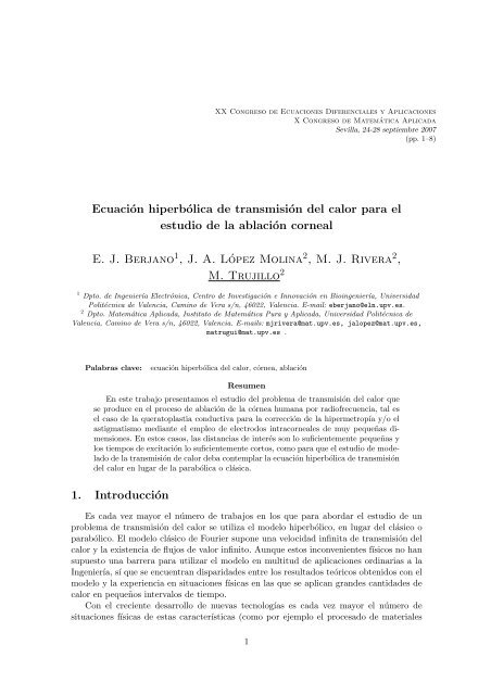
XX Congreso <strong>de</strong> Ecuaciones Diferenciales y Aplicaciones<br />
X Congreso <strong>de</strong> Matemática Aplicada<br />
Sevil<strong>la</strong>, 24-28 septiembre 2007<br />
(pp. 1–8)<br />
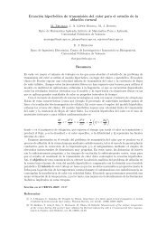
<strong>Ecuación</strong> <strong>hiperbólica</strong> <strong>de</strong> <strong>transmisión</strong> <strong>de</strong>l <strong>calor</strong> <strong>para</strong> <strong>el</strong><br />
<strong>estudio</strong> <strong>de</strong> <strong>la</strong> ab<strong>la</strong>ción corneal<br />
E. J. Berjano 1 , J. A. López Molina 2 , M. J. Rivera 2 ,<br />
M. Trujillo 2<br />
1 Dpto. <strong>de</strong> Ingeniería Electrónica, Centro <strong>de</strong> Investigación e Innovación en Bioingeniería, Universidad<br />
Politécnica <strong>de</strong> Valencia, Camino <strong>de</strong> Vera s/n, 46022, Valencia. E-mail: eberjano@<strong>el</strong>n.upv.es.<br />
2 Dpto. Matemática Aplicada, Instituto <strong>de</strong> Matemática Pura y Aplicada, Universidad Politécnica <strong>de</strong><br />
Valencia, Camino <strong>de</strong> Vera s/n, 46022, Valencia. E-mails: mjrivera@mat.upv.es, jalopez@mat.upv.es,<br />
matrugui@mat.upv.es .<br />
Pa<strong>la</strong>bras c<strong>la</strong>ve: ecuación <strong>hiperbólica</strong> <strong>de</strong>l <strong>calor</strong>, córnea, ab<strong>la</strong>ción<br />
Resumen<br />
En este trabajo presentamos <strong>el</strong> <strong>estudio</strong> <strong>de</strong>l problema <strong>de</strong> <strong>transmisión</strong> <strong>de</strong>l <strong>calor</strong> que<br />
se produce en <strong>el</strong> proceso <strong>de</strong> ab<strong>la</strong>ción <strong>de</strong> <strong>la</strong> córnea humana por radiofrecuencia, tal es<br />
<strong>el</strong> caso <strong>de</strong> <strong>la</strong> queratop<strong>la</strong>stia conductiva <strong>para</strong> <strong>la</strong> corrección <strong>de</strong> <strong>la</strong> hipermetropía y/o <strong>el</strong><br />
astigmatismo mediante <strong>el</strong> empleo <strong>de</strong> <strong>el</strong>ectrodos intracorneales <strong>de</strong> muy pequeñas dimensiones.<br />
En estos casos, <strong>la</strong>s distancias <strong>de</strong> interés son lo suficientemente pequeñas y<br />
los tiempos <strong>de</strong> excitación lo suficientemente cortos, como <strong>para</strong> que <strong>el</strong> <strong>estudio</strong> <strong>de</strong> mo<strong>de</strong><strong>la</strong>do<br />
<strong>de</strong> <strong>la</strong> <strong>transmisión</strong> <strong>de</strong> <strong>calor</strong> <strong>de</strong>ba contemp<strong>la</strong>r <strong>la</strong> ecuación <strong>hiperbólica</strong> <strong>de</strong> <strong>transmisión</strong><br />
<strong>de</strong>l <strong>calor</strong> en lugar <strong>de</strong> <strong>la</strong> <strong>para</strong>bólica o clásica.<br />
1. Introducción<br />
Es cada vez mayor <strong>el</strong> número <strong>de</strong> trabajos en los que <strong>para</strong> abordar <strong>el</strong> <strong>estudio</strong> <strong>de</strong> un<br />
problema <strong>de</strong> <strong>transmisión</strong> <strong>de</strong>l <strong>calor</strong> se utiliza <strong>el</strong> mo<strong>de</strong>lo hiperbólico, en lugar <strong>de</strong>l clásico o<br />
<strong>para</strong>bólico. El mo<strong>de</strong>lo clásico <strong>de</strong> Fourier supone una v<strong>el</strong>ocidad infinita <strong>de</strong> <strong>transmisión</strong> <strong>de</strong>l<br />
<strong>calor</strong> y <strong>la</strong> existencia <strong>de</strong> flujos <strong>de</strong> valor infinito. Aunque estos inconvenientes físicos no han<br />
supuesto una barrera <strong>para</strong> utilizar <strong>el</strong> mo<strong>de</strong>lo en multitud <strong>de</strong> aplicaciones ordinarias a <strong>la</strong><br />
Ingeniería, sí que se encuentran disparida<strong>de</strong>s entre los resultados teóricos obtenidos con <strong>el</strong><br />
mo<strong>de</strong>lo y <strong>la</strong> experiencia en situaciones físicas en <strong>la</strong>s que se aplican gran<strong>de</strong>s cantida<strong>de</strong>s <strong>de</strong><br />
<strong>calor</strong> en pequeños intervalos <strong>de</strong> tiempo.<br />
Con <strong>el</strong> creciente <strong>de</strong>sarrollo <strong>de</strong> nuevas tecnologías es cada vez mayor <strong>el</strong> número <strong>de</strong><br />
situaciones físicas <strong>de</strong> estas características (como por ejemplo <strong>el</strong> procesado <strong>de</strong> materiales<br />
1
E. J. Berjano, J. A. López Molina, M. J. Rivera, M. Trujillo<br />
mediante pulsos <strong>de</strong> láser o <strong>la</strong> irradiación <strong>el</strong>ectromagnética <strong>de</strong> sólidos). En estos casos <strong>el</strong><br />
empleo <strong>de</strong>l mo<strong>de</strong>lo hiperbólico subsana los errores <strong>de</strong>l clásico. El mo<strong>de</strong>lo hiperbólico supone<br />
una v<strong>el</strong>ocidad finita <strong>de</strong> <strong>transmisión</strong> <strong>de</strong>l <strong>calor</strong> y <strong>la</strong> existencia <strong>de</strong> flujos <strong>de</strong> valor finito. La<br />
ecuación <strong>hiperbólica</strong> <strong>de</strong>l <strong>calor</strong> en <strong>el</strong> caso <strong>de</strong> materiales isótropos es (ver [3])<br />
∂T<br />
∂t (x, t) + τ ∂2 <br />
T<br />
1<br />
(x, t) = α ∆T (x, t) + Q(x, t) + τ<br />
∂t2 ρc<br />
∂Q<br />
<br />
(x, t) , (1)<br />
∂t<br />
don<strong>de</strong> T es <strong>la</strong> temperatura, x y t <strong>la</strong> variables espacial y temporal, respectivamente, τ <strong>el</strong><br />
parámetro <strong>de</strong> r<strong>el</strong>ajación, ρ <strong>la</strong> <strong>de</strong>nsidad, c <strong>el</strong> <strong>calor</strong> específico, α <strong>la</strong> difusividad y Q <strong>la</strong>s fuentes<br />
internas <strong>de</strong> <strong>calor</strong>.<br />
Estamos interesados en <strong>el</strong> <strong>estudio</strong> <strong>de</strong>l problema <strong>de</strong> <strong>transmisión</strong> <strong>de</strong>l <strong>calor</strong> que se produce<br />
en <strong>el</strong> proceso <strong>de</strong> ab<strong>la</strong>ción <strong>de</strong> <strong>la</strong> córnea humana mediante radiofrecuencia, tal es <strong>el</strong> caso <strong>de</strong><br />
<strong>la</strong> queratop<strong>la</strong>stia conductiva <strong>para</strong> <strong>la</strong> corrección <strong>de</strong> <strong>la</strong> hipermetropía y/o <strong>el</strong> astigmatismo<br />
mediante <strong>el</strong> empleo <strong>de</strong> <strong>el</strong>ectrodos intracorneales <strong>de</strong> dimensiones muy pequeñas. En estos<br />
casos, <strong>la</strong>s distancias <strong>de</strong> interés son lo suficientemente pequeñas, y los tiempos <strong>de</strong> excitación<br />
lo suficientemente cortos, como <strong>para</strong> que <strong>el</strong> <strong>estudio</strong> <strong>de</strong> mo<strong>de</strong><strong>la</strong>do <strong>de</strong> <strong>la</strong> <strong>transmisión</strong> <strong>de</strong><br />
<strong>calor</strong> <strong>de</strong>ba contemp<strong>la</strong>r <strong>la</strong> ecuación <strong>hiperbólica</strong>. Así, <strong>el</strong> objetivo <strong>de</strong> esta comunicación<br />
es obtener <strong>la</strong> solución analítica <strong>de</strong>l problema <strong>de</strong> ab<strong>la</strong>ción en <strong>la</strong> cornea bajo <strong>el</strong> punto <strong>de</strong><br />
vista <strong>de</strong>l mo<strong>de</strong>lo hiperbólico y com<strong>para</strong>r<strong>la</strong> con <strong>la</strong> obtenida con <strong>el</strong> mo<strong>de</strong>lo <strong>para</strong>bólico. El<br />
interés <strong>de</strong> este trabajo se basa en que los mo<strong>de</strong>los matemáticos propuestos hasta <strong>la</strong> fecha<br />
<strong>para</strong> <strong>la</strong> predicción <strong>de</strong> <strong>la</strong> temperatura corneal durante <strong>el</strong> calentamiento con radiofrecuencia<br />
no contemp<strong>la</strong>n <strong>la</strong> transferencia <strong>de</strong> <strong>calor</strong> con v<strong>el</strong>ocidad finita. El mo<strong>de</strong>lo que presentamos<br />
permitirá una mejor estimación <strong>de</strong> <strong>la</strong> temperatura, y por lo tanto, una mejora en <strong>la</strong><br />
comprensión <strong>de</strong> los fenómenos biofísicos implicados en estas terapias.<br />
2. P<strong>la</strong>nteamiento <strong>de</strong>l problema<br />
Con objeto <strong>de</strong> po<strong>de</strong>r abordar <strong>el</strong> problema <strong>de</strong> forma analítica hemos consi<strong>de</strong>rado un<br />
mo<strong>de</strong>lo que supone una simplificación <strong>de</strong>l escenario real. En concreto hemos consi<strong>de</strong>rado<br />
un <strong>el</strong>ectrodo activo esférico <strong>de</strong> radio 45 micras, incrustado en <strong>el</strong> tejido corneal que se<br />
supone <strong>de</strong> extensión infinita. En un punto en <strong>el</strong> infinito se situaría <strong>el</strong> <strong>el</strong>ectrodo dispersivo.<br />
Es natural en <strong>el</strong> problema que vamos a estudiar <strong>el</strong> empleo <strong>de</strong> coor<strong>de</strong>nadas esféricas<br />
en <strong>la</strong> ecuación (1), siendo todas <strong>la</strong>s variables in<strong>de</strong>pendientes <strong>de</strong> los ángulos esféricos. La<br />
fuente <strong>de</strong> <strong>calor</strong> viene dada por <strong>la</strong> expresión<br />
Q(r, t) =<br />
P r0<br />
H(t) ,<br />
4πr4 don<strong>de</strong> H(t) es <strong>la</strong> función <strong>de</strong> Heavisi<strong>de</strong>, P <strong>la</strong> energía aplicada y r0 <strong>el</strong> radio <strong>de</strong>l <strong>el</strong>ectrodo.<br />
Así, <strong>la</strong> ecuación <strong>de</strong> gobierno <strong>de</strong>l problema es<br />
<br />
∂2T 2 ∂T<br />
−α (r, t) +<br />
∂r2 r ∂r<br />
<br />
(r, t) + ∂T<br />
siendo k <strong>la</strong> conductividad térmica<br />
∂t (r, t) + τ ∂2T P α r0<br />
(r, t) =<br />
∂t2 4 π k r4 <br />
α = k<br />
<br />
ρc y δ(t) <strong>la</strong> distribución <strong>de</strong> Dirac.<br />
2<br />
<br />
<br />
H(t) + τδ(t) , (2)
<strong>Ecuación</strong> <strong>hiperbólica</strong> <strong>de</strong>l <strong>calor</strong> en <strong>la</strong> ab<strong>la</strong>ción corneal<br />
Las condiciones <strong>de</strong> iniciales y <strong>de</strong> contorno son<br />
T (r, 0) = T0 ,<br />
lím<br />
r→∞ T (r, t) = T0 ,<br />
∂T<br />
(r, 0) = 0 ∀r > r0<br />
∂t<br />
<br />
τ ρ0 c r0 1 ∂T<br />
3 k τ ∂t (r0, t) + ∂2T ∂t2 (r0,<br />
<br />
t) = ∂T<br />
∂r (r0, t) ∀ t > 0 . (3)<br />
Para obtener <strong>la</strong> última condición <strong>de</strong> (3), junto con <strong>la</strong> expresión <strong>de</strong>l flujo hiperbólico (ver<br />
[3]), se ha hecho una simplificación adicional consistente en suponer que <strong>la</strong> temperatura<br />
<strong>de</strong>l <strong>el</strong>ectrodo es constante en todos sus puntos, con lo que <strong>el</strong> <strong>calor</strong> que entra en él por<br />
unidad <strong>de</strong> tiempo se pue<strong>de</strong> calcu<strong>la</strong>r mediante <strong>la</strong> fórmu<strong>la</strong> <strong>el</strong>emental<br />
4πr<br />
ρ0c0<br />
3 0 ∂T<br />
3 ∂t (r0, t) ,<br />
siendo c0 y ρ0 <strong>el</strong> <strong>calor</strong> específico y <strong>la</strong> <strong>de</strong>nsidad <strong>de</strong>l <strong>el</strong>ectrodo. Adimensionalizamos <strong>el</strong> problema<br />
utilizando <strong>la</strong>s siguientes variables<br />
ρ := r<br />
r0<br />
; ξ =<br />
α t<br />
r 2 0<br />
; λ =<br />
α τ<br />
r 2 0<br />
; V (ρ, ξ) =<br />
4 π k r0<br />
P<br />
<br />
T r0 ρ, r2 0 ξ<br />
<br />
− T0<br />
α<br />
don<strong>de</strong> T0 es <strong>la</strong> temperatura ambiente. La formu<strong>la</strong>ción <strong>de</strong>l problema adimensional es<br />
V (ρ, 0) = 0 ,<br />
<br />
∂2V 2<br />
− +<br />
∂ρ2 ρ<br />
lím V (ρ, ξ) = 0 ,<br />
ρ→∞<br />
<br />
∂V<br />
+<br />
∂ρ<br />
∂V<br />
∂ξ + λ ∂2V 1<br />
=<br />
∂ξ2 ρ4 <br />
<br />
H(ξ) + λ δ(ξ)<br />
∂V<br />
(ρ, 0) = 0<br />
∂ξ<br />
∀ρ > 1 (5)<br />
∂V<br />
∂ξ (1, ξ) + λ ∂2V ∂ξ2 3 ∂V<br />
(1, ξ) = (1, ξ)<br />
m ∂ρ<br />
∀ ξ > 0 , (6)<br />
siendo m = ρ0 c0<br />
ρc . Tomando transformadas <strong>de</strong> Lap<strong>la</strong>ce L(ρ, s) := Lξ[V (ρ, ξ](ρ, s) respecto<br />
a ξ obtenemos<br />
<br />
∂2L 2<br />
− +<br />
∂ρ2 ρ<br />
<br />
∂L<br />
+ (s + λ s<br />
∂ρ<br />
2 ) L = 1<br />
ρ4 <br />
1<br />
+ λ<br />
s<br />
lím<br />
ρ→∞ L(ρ, s) = 0 , (s + λs2 )L(1, s) = 3<br />
m<br />
;<br />
(4)<br />
(7)<br />
∂L<br />
(1, s). (8)<br />
∂ρ<br />
Utilizando <strong>la</strong> nueva función z(ρ, s) := ρ L(ρ, s) y <strong>el</strong> método <strong>de</strong> variación <strong>de</strong> <strong>la</strong>s constantes<br />
llegamos a <strong>la</strong> solución general <strong>de</strong> (7)<br />
√<br />
A(s) ρ e<br />
ρ<br />
<br />
1<br />
L = −<br />
2 ρ 1 e<br />
+ λ<br />
A(s) s 1<br />
−√A(s) u<br />
u3 <br />
du + M1(s)<br />
<br />
1<br />
+<br />
2 √<br />
ρ A(s) u<br />
1 e<br />
+ λ<br />
A(s) s u3 <br />
e<br />
du + M2(s)<br />
−√A(s) ρ<br />
, (9)<br />
ρ<br />
1<br />
3
E. J. Berjano, J. A. López Molina, M. J. Rivera, M. Trujillo<br />
don<strong>de</strong> A(s) = s + λ s2 y M1(s) y M2(s) son funciones que verifican <strong>la</strong>s condiciones <strong>de</strong><br />
contorno (8)<br />
√<br />
∞ A(s) u e<br />
+ λ<br />
1 u3 1<br />
M1(s) =<br />
2 <br />
1<br />
du<br />
A(s) s<br />
M2(s) = − e2 √ A(s)<br />
2 <br />
1 mA(s) − 3 A(s) + 3<br />
+ λ<br />
A(s) s mA(s) + 3 ∞ e<br />
A(s) + 3<br />
−√A(s) u<br />
u3 du.<br />
Introduciendo <strong>el</strong> valor <strong>de</strong> estas funciones en (9), <strong>la</strong> temperatura adimensional será <strong>la</strong><br />
transformada inversa <strong>de</strong> Lap<strong>la</strong>ce<br />
V (ρ, ξ) : = L −1<br />
<br />
1 1<br />
s<br />
+ λ<br />
2 ρ s √<br />
A(s) ρ ∞<br />
e<br />
e<br />
<br />
A(s) ρ<br />
−√A(s) u<br />
u3 du + e−√A(s) ρ<br />
<br />
A(s)<br />
√<br />
ρ A(s) u e<br />
×<br />
u3 du − e 2 √ A(s) mA(s) − 3A(s) + 3<br />
mA(s) + 3 ∞ e<br />
A(s) + 3<br />
−√A(s) u<br />
u3 <br />
du<br />
1<br />
= L −1 [F1] + L −1 [F2] − L −1 [F3]. (10)<br />
Así, tenemos que calcu<strong>la</strong>r <strong>la</strong> transformada inversa <strong>de</strong> F1, F2 y F3. En primer lugar<br />
L −1 [F1] = L −1<br />
√<br />
A(s)ρ e<br />
2ρ ∞<br />
1<br />
e<br />
+ λ<br />
A(s) s ρ<br />
−√A(s)u u3 <br />
du<br />
<br />
∞<br />
= L −1<br />
√ <br />
A(s)(ρ−u)<br />
1 e<br />
+ λL<br />
s A(s)<br />
−1<br />
√ <br />
A(s)(ρ−u) e<br />
du<br />
=<br />
A(s) 2ρu3 ρ<br />
y por <strong>el</strong> teorema <strong>de</strong> tras<strong>la</strong>ción <strong>de</strong> <strong>la</strong>s transformadas <strong>de</strong> Lap<strong>la</strong>ce y <strong>la</strong> fórmu<strong>la</strong> (36) <strong>de</strong> <strong>la</strong><br />
sección 5.6 <strong>de</strong>l capítulo 5 <strong>de</strong> [2]<br />
∞<br />
= H<br />
ρ<br />
ξ − √ <br />
ξ<br />
− 1 <br />
λ(u − ρ) λe 2λ I0 ξ2 − λ(u − ρ) 2<br />
2λ<br />
ξ<br />
<br />
v<br />
− 1 <br />
+ √ e 2 λ I0 v2 − λ(u − ρ) 2 dv<br />
λ(u−ρ) 2λ<br />
<br />
du<br />
2 √ =<br />
λ ρu3 ρ+ √λ<br />
ξ <br />
ξ<br />
− 1 <br />
= λe 2λ I0 ξ2 − λ(u − ρ) 2<br />
ρ<br />
2λ<br />
ξ<br />
<br />
v<br />
− 1 <br />
+ e 2 λ I0 v2 − λ(u − ρ) 2 dv<br />
2λ<br />
<br />
du<br />
2 √ . (11)<br />
λ ρu3 √ λ(u−ρ)<br />
Procediendo <strong>de</strong> forma análoga al cálculo <strong>de</strong> <strong>la</strong> inversa <strong>de</strong> F1 obtenemos<br />
L −1 ρ <br />
[F2] = H ξ −<br />
1<br />
√ <br />
λ(ρ − u)<br />
<br />
ξ<br />
− 1 <br />
λ e 2 λ I0 ξ2 − λ(ρ − u) 2<br />
2λ<br />
ξ<br />
<br />
v<br />
− 1 du<br />
+ e 2λ I0 v2 − λ(ρ − u) 2 dv<br />
2λ<br />
2 √ =<br />
λ ρ u3 √ λ(ρ−u)<br />
4<br />
1<br />
1
= H<br />
<strong>Ecuación</strong> <strong>hiperbólica</strong> <strong>de</strong>l <strong>calor</strong> en <strong>la</strong> ab<strong>la</strong>ción corneal<br />
<br />
ρ − ξ<br />
ρ<br />
√ − 1<br />
λ ρ− ξ<br />
<br />
ξ<br />
− 1<br />
λ e 2 λ I0<br />
√ 2λ<br />
λ<br />
<br />
<br />
ξ2 − λ(ρ − u) 2<br />
ξ<br />
<br />
v<br />
− 1 du<br />
+ √ e 2λ I0 v2 − λ(ρ − u) 2 dv<br />
λ(ρ−u) 2λ<br />
2 √ λ ρ u3 ρ <br />
ξ<br />
ξ<br />
− 1 <br />
+ H √λ − ρ + 1 λ e 2 λ I0 ξ2 − λ(ρ − u) 2<br />
1<br />
2λ<br />
ξ<br />
<br />
v<br />
− 1 du<br />
+ √ e 2λ I0 v2 − λ(ρ − u) 2 dv<br />
λ(ρ−u) 2λ<br />
2 √ λ ρ u3 don<strong>de</strong> I0(z) <strong>de</strong>nota <strong>la</strong> función modificada <strong>de</strong> Bess<strong>el</strong> <strong>de</strong> or<strong>de</strong>n 0.<br />
El cálculo <strong>de</strong> L−1 [F3] resulta ser <strong>el</strong> más complicado y sutil <strong>de</strong>l artículo. Para <strong>el</strong>lo se<br />
utiliza <strong>el</strong> teorema <strong>de</strong> convolución en <strong>la</strong> forma<br />
1 <br />
1<br />
− e<br />
+ λ<br />
√ A(s)(u+ρ−2)<br />
<br />
A(s)<br />
L −1 ∞<br />
[F3] = L<br />
1<br />
−1<br />
mA(s) − 3<br />
s A(s) + 3<br />
mA(s) + 3 du<br />
A(s) + 3 2ρ u3 <br />
∞<br />
= L −1<br />
<br />
e−√ <br />
A(s)(u+ρ−2)<br />
∗ L<br />
A(s)<br />
−1<br />
1 <br />
+ λ<br />
s <br />
6<br />
1 −<br />
A(s)<br />
mA(s) + 3 <br />
du<br />
.<br />
A(s) + 3 2ρu3 La primera inversa que aparece en <strong>la</strong> expresión anterior es<br />
G(ρ, ξ, u) : = L −1<br />
<br />
= H<br />
= H<br />
<br />
e−√ <br />
A(s)(u+ρ−2)<br />
<br />
A(s)<br />
− ξ<br />
2λ<br />
<br />
1 <br />
ξ2 − λ(u + ρ − 2) 2<br />
2λ<br />
(12)<br />
ξ − √ λ u + ρ − 2 e √ I0<br />
λ<br />
<br />
ξ − √ λ u + ρ − 2 <br />
G1(ρ, ξ, u) . (13)<br />
Para calcu<strong>la</strong>r <strong>la</strong> segunda inversa<br />
L −1<br />
1 <br />
+ λ<br />
s <br />
6<br />
1 −<br />
A(s)<br />
mA(s) + 3 <br />
A(s) + 3<br />
= 1 + λδ(ξ) − L −1<br />
1 <br />
6<br />
+ λ<br />
s A(s)<br />
mA(s) + 3 <br />
A(s) + 3<br />
utilizamos <strong>la</strong> fórmu<strong>la</strong> <strong>de</strong> Bromwich, mediante <strong>el</strong> circuito habitual en <strong>el</strong> caso <strong>de</strong> tener puntos<br />
<strong>de</strong> ramificación. En nuestro caso tales puntos son s = 0 y s = −1/λ y a<strong>de</strong>más existen dos<br />
polos simples<br />
s1 = 1<br />
<br />
−m − m<br />
2λm<br />
2 + 2λ 9 − 6m + √ 81 − 108m <br />
s2 = 1<br />
<br />
−m − m<br />
2λm<br />
2 + 2λ 9 − 6m − √ 81 − 108m <br />
.<br />
5
E. J. Berjano, J. A. López Molina, M. J. Rivera, M. Trujillo<br />
interiores al contorno <strong>de</strong> Bromwich. Obsérvese que s1 y s2 son números reales si 0 ≤ m < 3<br />
4 .<br />
Como <strong>la</strong>s situaciones prácticas más frecuentes están cubiertas con este caso, a partir <strong>de</strong><br />
ahora supondremos que <strong>el</strong> valor <strong>de</strong> m está en este intervalo. L<strong>la</strong>mando<br />
r1 = 1<br />
√ 2m<br />
<br />
9 − 6m + √ 81 − 108m ; r2 = 1<br />
√ 2m<br />
<br />
9 − 6m − √ 81 − 108m<br />
y utilizando <strong>el</strong> teorema <strong>de</strong> los residuos se obtiene<br />
R(ξ) : = L −1<br />
1 <br />
6<br />
+ λ<br />
s A(s)<br />
mA(s) + 3 <br />
2<br />
= −12 e<br />
A(s) + 3<br />
k=1<br />
sk ξ (1 + λ sk)r2 k<br />
sk(1 + 2λ sk)(2rkm − 3)<br />
− 6<br />
0<br />
π − 1<br />
√<br />
s ξ 1 + λ s m(s + λs2 ) + 3 −s − λs2 e<br />
s (m(s + λs<br />
λ<br />
2 ) + 3) 2 − (s + λs2 ds .<br />
)<br />
De (13) se tiene que<br />
G(ρ, ξ, u) ∗ 1 + λ δ(ξ) − R(ξ) ξ<br />
= G(ρ, ξ − v, u)(1 + λδ(v) − R(v) dv<br />
y por tanto<br />
L −1 ∞<br />
[F3] =<br />
1<br />
= H<br />
+<br />
<br />
ξ<br />
λG(ρ, ξ, u) +<br />
ξ<br />
√λ − ρ + 1<br />
ξ− √ λ(u+ρ−2)<br />
0<br />
0<br />
ξ<br />
= λG(ρ, ξ, u) + G(ρ, ξ − v, u) 1 − R(v) dv<br />
0<br />
ξ<br />
√λ −ρ+2<br />
1<br />
0<br />
G(ρ, ξ − v, u) 1 − R(v) <br />
du<br />
dv<br />
2ρu3 G1(ρ, ξ, u) 1 − R(v) dv<br />
(λ G1(ρ, ξ, u)<br />
<br />
du<br />
. (14)<br />
2ρu3 Concluyendo, <strong>la</strong> temperatura adimensional que queríamos calcu<strong>la</strong>r V (ρ, ξ, λ, m) se obtiene<br />
a partir <strong>de</strong> (10), (11), (12) y (14).<br />
3. Com<strong>para</strong>ción con <strong>el</strong> mo<strong>de</strong>lo <strong>para</strong>bólico<br />
Para com<strong>para</strong>r los resultados anteriores con los obtenidos con <strong>el</strong> mo<strong>de</strong>lo clásico <strong>de</strong><br />
Fourier calcu<strong>la</strong>mos <strong>la</strong> temperatura <strong>para</strong>bólica TF (r, t, m) <strong>para</strong> <strong>el</strong> mismo problema. Utilizando<br />
<strong>la</strong>s mismas variables adimensionales ρ y ξ, <strong>la</strong> temperatura adimensional <strong>de</strong> Fourier<br />
VF (ρ, ξ, m) es <strong>la</strong> solución <strong>de</strong>l problema<br />
V (ρ, 0) = 0 ,<br />
−<br />
lím V (ρ, ξ) = 0 ,<br />
ρ→∞<br />
<br />
∂2V 2<br />
+<br />
∂ρ2 ρ<br />
<br />
∂V<br />
+<br />
∂ρ<br />
∂V<br />
∂ξ<br />
= 1<br />
ρ 4<br />
∂V<br />
(ρ, 0) = 0 ∀ρ > 1<br />
∂ξ<br />
∂V 3<br />
(1, ξ) =<br />
∂ξ m<br />
6<br />
∂V<br />
(1, ξ) ∀ t > 0 .<br />
∂ρ
<strong>Ecuación</strong> <strong>hiperbólica</strong> <strong>de</strong>l <strong>calor</strong> en <strong>la</strong> ab<strong>la</strong>ción corneal<br />
Utilizando los mismos métodos que en <strong>el</strong> caso hiperbólico obtenemos (si 0 ≤ m < 3<br />
4 )<br />
∞ 1<br />
VF (ρ, t, m) =<br />
1 2ρu3 ⎛<br />
⎞<br />
(u−ρ)2<br />
ξ −<br />
⎝<br />
e 4v<br />
√ dv⎠<br />
du<br />
0 πv<br />
1<br />
2ρu3 ⎛<br />
<br />
ξ<br />
⎝ 1 − 6<br />
∞ (3 − my) e<br />
π<br />
−y(ξ−v)<br />
<br />
√ dy<br />
y(m2y2 + (9 − 6m)y + 9)<br />
∞<br />
−<br />
1<br />
0<br />
4. Resultados y conclusiones<br />
0<br />
⎞<br />
(u+ρ−2)2<br />
− e 4v<br />
√ ⎠ dv .<br />
πv<br />
En <strong>la</strong>s simu<strong>la</strong>ciones empleamos <strong>la</strong> características <strong>el</strong>éctricas y técnicas <strong>de</strong> <strong>la</strong> córnea <strong>de</strong><br />
un trabajo previo [1] y <strong>el</strong> tiempo <strong>de</strong> r<strong>el</strong>ajación térmica <strong>de</strong> 0,1 s. Suponemos un <strong>el</strong>ectrodo<br />
<strong>de</strong> p<strong>la</strong>tino [4]. La potencia aplicada fue <strong>de</strong> 30 mW durante 600 ms y <strong>la</strong> temperatura inicial<br />
35 ◦ C.<br />
La figura 1 muestra que al comienzo <strong>de</strong>l calentamiento con <strong>la</strong> ecuación <strong>para</strong>bólica se<br />
obtienen valores más bajos <strong>de</strong> temperatura que con <strong>la</strong> <strong>hiperbólica</strong>, lo cual es altamente r<strong>el</strong>evante<br />
en <strong>la</strong>s aplicaciones quirúrgicas. Des<strong>de</strong> <strong>el</strong> punto <strong>de</strong> vista matemático, es significativa<br />
<strong>la</strong> presencia <strong>de</strong> singu<strong>la</strong>rida<strong>de</strong>s <strong>de</strong> <strong>la</strong> solución localizadas a lo <strong>la</strong>rgo <strong>de</strong> <strong>la</strong> recta (en variables<br />
adimensionales) ξ = √ λ(ρ − 1), que refleja <strong>la</strong> naturaleza <strong>hiperbólica</strong> <strong>de</strong> <strong>la</strong> ecuación <strong>de</strong><br />
gobierno (2).<br />
90<br />
80<br />
70<br />
60<br />
50<br />
40<br />
T<br />
t0.01<br />
t0.03<br />
t0.05<br />
t0.01<br />
t0.03<br />
t0.05<br />
0.00006 0.00008 0.0001 0.00012 0.00014 0.00016 0.00018 r<br />
Figura 1: Temperaturas <strong>de</strong> <strong>la</strong> córnea (<strong>hiperbólica</strong> trazo continuo, Fourier discontinuo)<br />
<strong>de</strong>s<strong>de</strong> r = 45 10 −6 m hasta r = 185 10 −6 m en diferentes tiempos.<br />
Agra<strong>de</strong>cimientos<br />
Este trabajo ha sido financiado parcialmente por <strong>el</strong> MEC y <strong>la</strong> FEDER, Proyecto<br />
MTM2004-02262 y <strong>la</strong> red <strong>de</strong> investigación MTM2006-26627-E, <strong>el</strong> ”P<strong>la</strong>n Nacional <strong>de</strong> Investigación<br />
Científica, Desarrollo e Innovación Tecnológica <strong>de</strong>l Ministerio <strong>de</strong> Educación y<br />
Ciencia”<strong>de</strong> España (TEC 2005-04199/TCM) y <strong>el</strong> Programa <strong>de</strong> Apoyo a <strong>la</strong> Investigación y<br />
Desarrollo (PAID-04-07) <strong>de</strong> <strong>la</strong> UPV.<br />
7
Referencias<br />
E. J. Berjano, J. A. López Molina, M. J. Rivera, M. Trujillo<br />
[1] E. J. Berjano, J. L. Alio & J. Saiz, Mo<strong>de</strong>ling for radio-frequency conductive keratop<strong>la</strong>sty: implications<br />
for the maximum temperature reached in the cornea, Physiol. Meas. 26, (2005), 157-172.<br />
[2] A. Erdélyi, M. F. Oberhettinger & F. G. Tricomi, Tables of Integral Transforms. Vol. I and II,<br />
McGraw-Hill, New York, 1954.<br />
[3] M. N. Özi¸sik & D. T. Tzou, On the wave theory in heat conduction, ASME Journal of Heat Transfer,<br />
116, (1994) 526-535.<br />
[4] D. Panescu, J. G. Whayne, S. D. Fleishman, M. S. Mirotznik, D. K. Swanson & J. G. Webster Threedimensional<br />
finite analysis of current <strong>de</strong>nsity and temperature distributions during radio-frequency<br />
ab<strong>la</strong>tion, IEEE Trans. Biomed. Eng., 42, (1995), 879-890.<br />
8