Ecuación hiperbólica de transmisión del calor para el estudio de la ...

E. J. Berjano, J. A. López Molina, M. J. Rivera, M. Trujillo
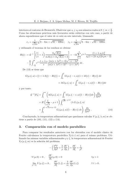
interiores al contorno de Bromwich. Obsérvese que s1 y s2 son números reales si 0 ≤ m < 3
4 .
Como las situaciones prácticas más frecuentes están cubiertas con este caso, a partir de
ahora supondremos que el valor de m está en este intervalo. Llamando
r1 = 1
√ 2m
9 − 6m + √ 81 − 108m ; r2 = 1
√ 2m
9 − 6m − √ 81 − 108m
y utilizando el teorema de los residuos se obtiene
R(ξ) : = L −1
1
6
+ λ
s A(s)
mA(s) + 3
2
= −12 e
A(s) + 3
k=1
sk ξ (1 + λ sk)r2 k
sk(1 + 2λ sk)(2rkm − 3)
− 6
0
π − 1
√
s ξ 1 + λ s m(s + λs2 ) + 3 −s − λs2 e
s (m(s + λs
λ
2 ) + 3) 2 − (s + λs2 ds .
)
De (13) se tiene que
G(ρ, ξ, u) ∗ 1 + λ δ(ξ) − R(ξ) ξ
= G(ρ, ξ − v, u)(1 + λδ(v) − R(v) dv
y por tanto
L −1 ∞
[F3] =
1
= H
+
ξ
λG(ρ, ξ, u) +
ξ
√λ − ρ + 1
ξ− √ λ(u+ρ−2)
0
0
ξ
= λG(ρ, ξ, u) + G(ρ, ξ − v, u) 1 − R(v) dv
0
ξ
√λ −ρ+2
1
0
G(ρ, ξ − v, u) 1 − R(v)
du
dv
2ρu3 G1(ρ, ξ, u) 1 − R(v) dv
(λ G1(ρ, ξ, u)
du
. (14)
2ρu3 Concluyendo, la temperatura adimensional que queríamos calcular V (ρ, ξ, λ, m) se obtiene
a partir de (10), (11), (12) y (14).
3. Comparación con el modelo parabólico
Para comparar los resultados anteriores con los obtenidos con el modelo clásico de
Fourier calculamos la temperatura parabólica TF (r, t, m) para el mismo problema. Utilizando
las mismas variables adimensionales ρ y ξ, la temperatura adimensional de Fourier
VF (ρ, ξ, m) es la solución del problema
V (ρ, 0) = 0 ,
−
lím V (ρ, ξ) = 0 ,
ρ→∞
∂2V 2
+
∂ρ2 ρ
∂V
+
∂ρ
∂V
∂ξ
= 1
ρ 4
∂V
(ρ, 0) = 0 ∀ρ > 1
∂ξ
∂V 3
(1, ξ) =
∂ξ m
6
∂V
(1, ξ) ∀ t > 0 .
∂ρ