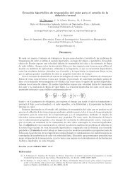
Ecuación hiperbólica de transmisión del calor para el estudio de la ...

Ecuación hiperbólica del calor en la ablación corneal
Las condiciones de iniciales y de contorno son
T (r, 0) = T0 ,
lím
r→∞ T (r, t) = T0 ,
∂T
(r, 0) = 0 ∀r > r0
∂t
τ ρ0 c r0 1 ∂T
3 k τ ∂t (r0, t) + ∂2T ∂t2 (r0,
t) = ∂T
∂r (r0, t) ∀ t > 0 . (3)
Para obtener la última condición de (3), junto con la expresión del flujo hiperbólico (ver
[3]), se ha hecho una simplificación adicional consistente en suponer que la temperatura
del electrodo es constante en todos sus puntos, con lo que el calor que entra en él por
unidad de tiempo se puede calcular mediante la fórmula elemental
4πr
ρ0c0
3 0 ∂T
3 ∂t (r0, t) ,
siendo c0 y ρ0 el calor específico y la densidad del electrodo. Adimensionalizamos el problema
utilizando las siguientes variables
ρ := r
r0
; ξ =
α t
r 2 0
; λ =
α τ
r 2 0
; V (ρ, ξ) =
4 π k r0
P
T r0 ρ, r2 0 ξ
− T0
α
donde T0 es la temperatura ambiente. La formulación del problema adimensional es
V (ρ, 0) = 0 ,
∂2V 2
− +
∂ρ2 ρ
lím V (ρ, ξ) = 0 ,
ρ→∞
∂V
+
∂ρ
∂V
∂ξ + λ ∂2V 1
=
∂ξ2 ρ4
H(ξ) + λ δ(ξ)
∂V
(ρ, 0) = 0
∂ξ
∀ρ > 1 (5)
∂V
∂ξ (1, ξ) + λ ∂2V ∂ξ2 3 ∂V
(1, ξ) = (1, ξ)
m ∂ρ
∀ ξ > 0 , (6)
siendo m = ρ0 c0
ρc . Tomando transformadas de Laplace L(ρ, s) := Lξ[V (ρ, ξ](ρ, s) respecto
a ξ obtenemos
∂2L 2
− +
∂ρ2 ρ
∂L
+ (s + λ s
∂ρ
2 ) L = 1
ρ4
1
+ λ
s
lím
ρ→∞ L(ρ, s) = 0 , (s + λs2 )L(1, s) = 3
m
;
(4)
(7)
∂L
(1, s). (8)
∂ρ
Utilizando la nueva función z(ρ, s) := ρ L(ρ, s) y el método de variación de las constantes
llegamos a la solución general de (7)
√
A(s) ρ e
ρ
1
L = −
2 ρ 1 e
+ λ
A(s) s 1
−√A(s) u
u3
du + M1(s)
1
+
2 √
ρ A(s) u
1 e
+ λ
A(s) s u3
e
du + M2(s)
−√A(s) ρ
, (9)
ρ
1
3