Solución del Control de Informática Gráfica - Noviembre 2010 ... - DAC

Solución del Control de Informática Gráfica - Noviembre 2010
Informática Gráfica, Curso 2010-2011 Control Noviembre
Miguel A. Otaduy
1 Ejercicio de Curvas
Transformaciones Geométricas, Curvas y Superficies
Control del 5 de Noviembre de 2010
1.1 Se ha de diseñar una curva cerrada que interpole 4 puntos con continuidad
C1 Ejercicio 1. (5 puntos)
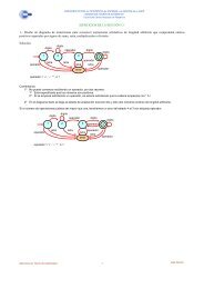
Apartado 1.a Se ha de diseñar una curva cerrada que interpole 4 puntos con continuidad
C
y con el menor grado posible. Como se muestra en la
figura, los puntos a interpolar son p0(t = 0) = (1, 0); p1(t = 1) = (2, 1);
p2(t = 2) = (1, 2); p3(t = 3) = (0, 1); y vuelta a p0(t = 4) = (1, 0).
1 y con el menor grado posible. Como se muestra en la figura, los puntos a interpolar
son p0 (t = 0) = (1, 0); p1 (t = 1) = (2, 1); p2 (t = 2) = (1, 2); p3 (t = 3) = (0, 1); y vuelta a
p0 (t = 4) = (1, 0).
p3 (t = 3) = (0,1)
p2 (t = 2) = (1,2)
p0 (t = 0, t = 4) = (1,0)
p1 (t = 1) = (2,1)
Nota: para obtener los coeficientes hay que resolver un sistema de ecuaciones. Será
Nota: suficiente para obtener con dejar los coeficientes ese sistema indicado, hay queno resolver hay por un qué sistema resolverlo. de ecuaciones. Será suficiente
con
Apartado
dejar ese
1.b
sistema
La curva
indicado,
del apartado
no hay
anterior
por qué
carece
resolverlo.
de una propiedad deseada. ¿Cuál es?
Decisión Indica delotros tipo posibles de curva: tipos de curvas con los que sí se obtendría esa propiedad, ¿pero qué
Decidiremos propiedad el tipo se perdería de curva en en ese función caso? de las propiedades a cumplir:
1. Ha de interpolar. (Quedan descartadas Bézier y B-splines.)
2. Ha de ser del menor grado posible. (Entre las curvas que interpolan, la de menor grado
posible es la spline.)
3. Ha de tener continuidad C 1 . (Este nivel de continuidad se puede obtener con una spline
cuadrática.)
Análisis del problema:
Una vez que hemos optado por la spline cuadrática, analizaremos su diseño. La curva spline
viene dividida en tramos (4 tramos en nuestro caso), y en cada tramo utilizaremos un polinomio
de grado 2 x(t) para definir la coordenada x, y un polinomio de grado 2 y(t) para definir la
coordenada y. Las coordenadas x e y se pueden tratar completamente por separado.
Para la coordenada x, por cada tramo tendremos 3 coeficientes a calcular, es decir, un total
de 12 incógnitas. Vamos a analizar cuántas condiciones de interpolación y continuidad podemos
formular para así calcular las incógnitas. La interpolación de los 5 puntos, {p0(t = 0), p1(t =
1), p2(t = 2), p3(t = 3), p0(t = 4)}, define 2 condiciones de interpolación por tramo, es decir 8

condiciones. La continuidad de la primera derivada en los 4 puntos de unión de tramos define 4
condiciones más. Por lo tanto, tenemos 12 condiciones para 12 incógnitas, y el problema se puede
resolver de manera exacta. En una curva abierta no habríamos tenido suficientes condiciones, pero
la condición de continuidad en el punto donde se cierra la curva permite definir perfectamente el
problema.
Este análisis de ecuaciones e incógnitas se podría hacer también para la coordenada y.
Definiciones de los polinomios y sus derivadas en cada tramo:
Primer tramo:
Segundo tramo:
Tercer tramo:
Cuarto tramo:
x = x10t 2 + x11t + x12
y = y10t 2 + y11t + y12
x = x20t 2 + x21t + x22
y = y20t 2 + y21t + y22
x = x30t 2 + x31t + x32
y = y30t 2 + y31t + y32
x = x40t 2 + x41t + x42
y = y40t 2 + y41t + y42
Condiciones de interpolación:
Primer tramo:
Segundo tramo:
x ′ = 2x10t + x11
y ′ = 2y10t + y11
x ′ = 2x20t + x21
y ′ = 2y20t + y21
x ′ = 2x30t + x31
y ′ = 2y30t + y31
x ′ = 2x40t + x41
y ′ = 2y40t + y41
x(0) = 1 ⇒ x12 = 1 x(1) = 2 ⇒ x10 + x11 + x12 = 2
y(0) = 0 ⇒ y12 = 0 y(1) = 1 ⇒ y10 + y11 + y12 = 1
x(1) = 2 ⇒ x20 + x21 + x22 = 2 x(2) = 1 ⇒ 4x20 + 2x21 + x22 = 1
y(1) = 1 ⇒ y20 + y21 + y22 = 1 y(2) = 2 ⇒ 4y20 + 2y21 + y22 = 2
Tercer tramo:
x(2) = 1 ⇒ 4x30 + 2x31 + x32 = 1 x(3) = 0 ⇒ 9x30 + 3x31 + x32 = 0
y(2) = 2 ⇒ 4y30 + 2y31 + y32 = 2 y(3) = 1 ⇒ 9y30 + 3y31 + y32 = 1
Cuarto tramo:
x(3) = 0 ⇒ 9x40 + 3x41 + x42 = 0 x(4) = 1 ⇒ 16x40 + 4x41 + x42 = 1
y(3) = 1 ⇒ 9y40 + 3y41 + y42 = 1 y(4) = 0 ⇒ 16y40 + 4y41 + y42 = 0

Condiciones de continuidad de derivadas:
Primer y segundo tramos:
Segundo y tercer tramos:
Tercer y cuarto tramos:
Cuarto y primer tramos:
Sistema de ecuaciones completo en x:
Sistema de ecuaciones completo en y:
x ′ (1) ⇒ 2x10 + x11 = 2x20 + x21
y ′ (1) ⇒ 2y10 + y11 = 2y20 + y21
x ′ (2) ⇒ 4x20 + x21 = 4x30 + x31
y ′ (2) ⇒ 4y20 + y21 = 4y30 + y31
x ′ (3) ⇒ 6x30 + x31 = 6x40 + x41
y ′ (3) ⇒ 6y30 + y31 = 6y40 + y41
x ′ (4) = x ′ (0) ⇒ 8x40 + x41 = x11
y ′ (4) = y ′ (0) ⇒ 8y40 + y41 = y11
x12 = 1
x10 + x11 + x12 = 2
x20 + x21 + x22 = 2
4x20 + 2x21 + x22 = 1
4x30 + 2x31 + x32 = 1
9x30 + 3x31 + x32 = 0
9x40 + 3x41 + x42 = 0
16x40 + 4x41 + x42 = 1
2x10 + x11 = 2x20 + x21
4x20 + x21 = 4x30 + x31
6x30 + x31 = 6x40 + x41
8x40 + x41 = x11

y12 = 0
y10 + y11 + y12 = 1
y20 + y21 + y22 = 1
4y20 + 2y21 + y22 = 2
4y30 + 2y31 + y32 = 2
y30 + 3y31 + y32 = 1
9y40 + 3y41 + y42 = 1
16y40 + 4y41 + y42 = 0
2y10 + y11 = 2y20 + y21
4y20 + y21 = 4y30 + y31
6y30 + y31 = 6y40 + y41
8y40 + y41 = y11
1.2 La curva del apartado anterior carece de una propiedad deseada. Identifica
esa propiedad. Indica otros posibles tipos de curvas con los que
sí se obtendría esa propiedad, e identifica qué propiedad se perdería
en ese caso.
La spline cuadrática carece de control local. Esto implica que cambiar un punto de control
afecta a toda la curva.
Se podrían usar curvas cúbicas (p.ej. Hermite). En ese caso se perdería la propiedad de grado
mínimo, pasando a ser 3, con el consiguiente riesgo de oscilaciones. Si se quiere usar Hermite,
hay que tener cuidado, porque no se puede hacer una simple asignación de parámetros x = t. El
problema es que la curva es cerrada. Si se quiere usar Hermite, hay que hacer el diseño de x(t) e
y(t) por separado, igual que con la spline cuadrática, pero definiendo distintas condiciones sobre
las derivadas.
Se podrían usar B-splines cuadráticas. En ese caso se perdería la propiedad de interpolación.
Se podría conseguir interpolación en los extremos asignando nodos de la B-spline de la manera
adecuada, pero en los puntos de control interiores sólo se conseguiría aproximación.

2 Ejercicio de Transformaciones
Informática Gráfica, Curso 2010-2011 Control Noviembre
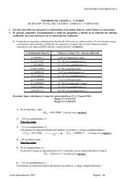
2.1 El Ejercicio rectángulo 2. (5 puntos) con textura de tetera de la imagen de la izquierda se ha
de transformar para que esté posicionado como en la imagen de la
El rectángulo con textura de tetera de la imagen de la izquierda se ha de transformar para
derecha. que esté posicionado La posición como en del la imagen centrode dela la derecha. textura La posición es en ambas del centro imágenes de la
(2.5, textura 2.5, es en 0), ambas y elimágenes rectángulo (2.5, 2.5, de0), lay textura el rectángulo está de colocado la textura está en colocado ambas en imágenes
ambas imágenes en el en plano el plano normal al vector (1, 1, (1, 0), 1, pero 0), la orientación pero la orientación y la escala han y la
escala cambiado. han cambiado.
X
A = (3,2,1)
D = (2,3,1)
(5,0,0) (0,5,0)
Z
B = (3,2,-1) C = (2,3,-1)
Y
D’ = (4,1,1)
A’ = (4,1,-1)
C’ = (1,4,1)
B’ = (1,4,-1)
Nota: Utilizar dibujos que ayuden a aclarar los distintos pasos efectuados. No es
Nota: necesario utilizarefectuar dibujoslas que multiplicaciones ayuden a aclarar entre los matrices distintos al expresar pasos efectuados. la transformación No esfinal, necesario
efectuar es las suficiente multiplicaciones con expresar entre cada matriz matrices y dejar al expresar el producto laindicado. transformación final, es suficiente
con expresar cada matriz y dejar el producto indicado.
Análisis del problema:
Para posicionar la textura como en la imagen final, hay dos transformaciones clave que se deben
aplicar: rotación de 90 grados alrededor del eje XY, y escalado. Para realizar estas dos operaciones
clave, realizaremos otra serie de transformaciones auxiliares: Por un lado, como el eje XY no
es uno de los ejes cartesianos, primero alinearemos el eje XY con uno de los ejes cartesianos,
realizaremos la rotación de 90 grados sobre ese eje, y luego desharemos la rotación inicial. Por
otro lado, como el escalado se ha de realizar respecto al origen, primero trasladaremos la textura
para centrarla en el origen de coordenadas, realizaremos el escalado allí, y luego desharemos la
traslación.
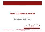
La secuencia de transformaciones seleccionada ha sido:
X
(5,0,0) (0,5,0)
1. R1: Rotar -45 grados alrededor del eje Z para alinear el eje XY con el eje X.
2. T2: Trasladar al origen.
3. R3: Rotar 90 grados alrededor del eje X.
4. S4: Escalar.
5. T5: Deshacer la traslación T2. T5 = T −1
2 .
6. R6: Deshacer la rotación R1. R6 = R −1
1 .
Z
Y

La transformación completa es:
M = R6T5S4R3T2R1
Hay muchas otras opciones para resolver el problema:
• Se puede alinear el eje XY con el eje Y en lugar del X.
• Se puede rotar para alinear antes de trasladar al origen.
• Se puede trasladar un vértice de la textura al origen en lugar de su centro, pero entonces hay
que tener cuidado al deshacer esta traslación. El escalado hace que la traslación final no sea
simplemente la inversa de la inicial.
Otras cuestiones importantes a tener en cuenta son que el escalado se ha de realizar en el origen,
no se puede escalar en el lugar donde se encuentra la textura. Y los escalados no son uniformes y
se han de calcular.
Rotación R1:
Rotación de -45 grados alrededor del eje Z:
R1 =
⎛
⎜
⎝
cos −45 − sin −45 0 0
sin −45 cos 45 0 0
0 0 1 0
0 0 0 1
⎞
⎟
⎠ =
⎛
⎜
⎝
(2)/2 (2)/2 0 0
− (2)/2 (2)/2 0 0
0 0 1 0
0 0 0 1
Traslación T2:
El punto (2.5, 2.5, 0) queda en (2.5 (2), 0, 0) después de la primera rotación. Se ha de
trasladar ese punto al origen:
T2 =
⎛
⎜
⎝
1 0 0 −2.5 (2)
0 1 0 0
0 0 1 0
0 0 0 1
Rotación R3:
Rotación de 90 grados alrededor del eje X:
⎛
1 0 0
⎞
0
⎜
R3 = ⎜ 0
⎝ 0
cos 90
sin 90
− sin 90
cos 90
0 ⎟
0 ⎠
0 0 0 1
=
⎛
1 0 0
⎞
0
⎜ 0
⎝ 0
0
1
−1
0
0 ⎟
0 ⎠
0 0 0 1
Escalado S4:
La textura original tiene tamaño 2 en el lado ancho y (2) en el lado estrecho. La textura final
tiene tamaño 3 (3) en el lado ancho y 2 en el lado estrecho. Dada la orientación actual de la
textura, requiere un escalado de (2) en el eje Z y 3/2 (2) en el eje Y. En el eje X se deja como
está (escalado 1).
⎛
⎞
S4 =
⎜
⎝
1
0
0
3/2
0 0
0
(2)
0
0
(2)
0
0
0 0 0 1
⎞
⎟
⎠
⎟
⎠
⎞
⎟
⎠

Traslación T5:
. Se consigue cambiando de signo al vector de traslación:
T5 = T −1
2
Rotación R6:
R6 = R −1
1 = RT 1 :
R6 =
T5 =
⎛
⎜
⎝
⎛
⎜
⎝
1 0 0 2.5 (2)
0 1 0 0
0 0 1 0
0 0 0 1
⎞
⎟
⎠
(2)/2 − (2)/2 0 0
(2)/2 (2)/2 0 0
0 0 1 0
0 0 0 1
⎞
⎟
⎠