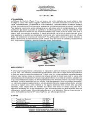
introducción a la mecánica analítica - fisica.ru

Enrique Cantera del Río Introducción a la Mecánica Analítica 18
S
S
1
2
:
( T1
− T3
) • dr
1 = 0 ⇒ T1
= T3
( T4
− T5
) • ( dr
4 − dr
3)
= 0⇒T4
= T5
:
Con estos resultados podemos aplicar la 2ª Ley de Newton al sistema y
obtener este sistema de ecuaciones
a + a = −(
a + a ); T = T ;
5
1
4
1
T = 2T
;
4
4
T − m g = m a ;
4
4
4
1
T − m g = m a ;
1
5
4
1
5
5
T − m g = m a ;
6 ecuaciones y 6 incógnitas que resuelven el problema. Note el lector que la
condición de equilibrio de las fuerzas de ligadura del principio de D´Alembert
también permite escribir el equilibrio de momentos para los subsistemas
S : r1
× T + r 2 × T + r 3 × T = 0
1
2
1
S : − r 3 × T + r 4 × T + r 5 × T = 0
3
y esto debe ser compatible con las conclusiones anteriores. Acto seguido
planteamos el Lagrangiano del sistema para resolver el problema según la
mecánica analítica
2
4
2 2 2
( m v + m v + m v ) − ( mgh + mgh mgh )
1
L = 1 1 4 4 5 5
1 4 +
2
de las restricciones geométricas, expresadas en términos de velocidades y
alturas, tenemos, en una dimensión:
v4
+ v5
+ 2v1
= 0
h + h + 2h
= h
4
donde h0 es una constante. Eliminando v1 y h1 en el Lagrangiano tenemos
5
2 2
1 ⎛ v
⎞
4 + v5
v4v5
2 2 ⎛ h0
− h4
− h5
⎞
L = ⎜
⎜m1
+ m1
+ m4v4
+ m5v5
⎟ − ⎜m1
g(
) + m4gh4
+ m5gh5
⎟
2 ⎝ 4 2
⎠ ⎝ 2
⎠
y las ecuaciones de Euler-Lagrange resultan
d ⎛ ∂L
⎞ ∂L
m1
m1
⎛ m1
⎞
− ≡ a + m + a = ⎜ − m ⎟g
dt ⎜
v ⎟
4(
4)
5(
)
4
⎝ ∂ 4 ⎠ ∂h4
4
4 ⎝ 2 ⎠
d ⎛ ∂L
⎞ ∂L
m1
m1
⎛ m1
⎞
− ≡ a + m + a = ⎜ − m ⎟g
dt ⎜
v ⎟
5(
5)
4(
)
5
⎝ ∂ 5 ⎠ ∂h5
4
4 ⎝ 2 ⎠
El lector puede comprobar que el sistema de ecuaciones obtenido
anteriormente por medio del principio de D´Alembert conduce a este mismo
resultado. En este ejemplo vemos las ecuaciones de Euler-Lagrange aplicadas
a un caso en que las fuerzas de ligadura producen un trabajo no nulo
individualmente, aunque nulo en conjunto. La justificación física de las
condiciones de equilibrio aplicadas a los dos subsistemas es que se consideran
1
0
3
5
1
5
1
5
5