El Control Robusto y el espacio de parámetros

EL CONTROL ROBUSTO
Y
EL ESPACIO DE PARÁMETROS
Roberto Hernández, Fernando Morilla
U.N.E.D.

RESULTADOS DE PUNTOS EXTREMOS
Teorema de Kharitonov, , 1978: intervalo de polinomios.
1 2
2
n
PI(, s q)
= q0 + qs
1
+ q2s + L + qns
n
− +
K
n i i i
q= ( q , q , , q ) ∈R , q ∈[ q , q ]
Necesario y suficiente: 4 polinomios distinguidos.
− +
i i i
0 < q ≤ q ≤ q
− − +
1 0 1 2 2 +
3 3 −
4 4 −
5 5 +
6 6
K ( s) = q + q s+ q s + q s + q s + q s + q s + ...;
+ + −
2 0 1 2 2 −
3 3 +
4 4 +
5 5 −
6 6
K ( s) = q + q s+ q s + q s + q s + q s + q s + ...;
+ − −
3 0 1 2 2 +
3 3 +
4 4 −
5 5 −
6 6
K ( s) = q + q s+ q s + q s + q s + q s + q s + ...;
− + +
4 0 1 2 2 −
3 3 −
4 4 +
5 5 +
6 6
K ( s) = q + q s+ q s + q s + q s + q s + q s + ...;
Olbrot, , 1983. Barmish.
CONTROL ROBUSTO: modelo de perturbaciones.
Estructuradas: se establecen en los parámetros de la planta.

∀n
• y se evita el mallado clásico
• Extensión a otros casos: discreto, comportamiento robusto, ...
■ POLITOPOS
RESULTADOS DE PUNTOS EXTREMOS
psq (, ) = s + a()
qs
Los coeficientes dependen de forma afín lineal de q
n
n−1
∑
i=
0
i
i
Teorema de la Arista, Teorema de Rantzer
ANÁLISIS: TEORÍA MADURA
(Barmish, 1993)
(Ackermann, 1993)
OBJETIVO: RESULTADOS PARA EL PROBLEMA DE DISEÑO

RESULTADOS DE PUNTOS EXTREMOS
Paradigma de intervalo de plantas:
⎧⎪
N (, s b)
P= Psab (, , ): Psab (, , ) = , N (, sb) ∈N, D(, sa)
∈D
⎪⎩
p
I ⎨
p
I P
I
Dp(, s a)
ut ()
+
-
Cs () =
Nc()
s
D () s
c
Cs () P (, sab , )
I
y()
t
⎫⎪
⎬
⎪⎭
δ ()= s N () s N (, s b) + D () s D (, s a)
I
c p c p
Politopo

RESULTADOS DE PUNTOS EXTREMOS
Resultados previos:
Ghosh, 1985: Controladores positivos, 4 polinomios.
Chapellat-Bhattacharyya, 1989: 32 aristas distinguidas.
Hollot y Yang, 1990: Controladores de 1er orden. Todas
las plantas extremas.
Barmish et al., 1992: Controladores de 1er orden. 16 plantas
de Kharitonov.
Djaferis, 1993: 64 polinomios virtuales.

RESULTADOS DE PUNTOS EXTREMOS
Hernández
ndez et al., 1995: 32 polinomios virtuales.
Se construyen en función n del controlador y de los polinomios de
Kharitonov del numerador y del denominador de la planta.
Propiedades y conservadurismo.
Hernández
ndez et al., 1996, Hernández
ndez et al., 1998: Generalización
del menor intervalo de polinomios que contiene al politopo de
polinomios.
Hernández
ndez et al., , 1999: : Generalización de los polinomios de
Bialas, , conservadurismo.

RESULTADOS DE PUNTOS EXTREMOS
CONCLUSIÓN: RPE PARA INTERVALO DE PLANTAS.
PROBLEMA: ESTABILIZAR UN POLINOMIO.
p()
s
n
= ∑cs
i
i=
0
i
p(
s,
k)
=
∑
∀i
/ i∈A
a s
i
i
+
∑
∀i
/ i∈K
k
i
s
i
Coeficientes constantes:
Parámetros:
A
K
{ a = c c = const}
i i i
{ = ≠ }
= /
= k c / c
i
i
i
const
OBJETIVO: : Determinar K, , si existe, tal que p(s,k) sea estable
ROUTH: 2 parámetros
Necesidad de resultados en el
espacio de parámetros.

ESPACIO DE PARÁMETROS
RESULTADOS OBTENIDOS:
Condiciones necesarias y suficientes para estabilizar un polinomio
en el espacio de parámetros:
EXISTENCIA DE SOLUCIÓN.
ALGORITMO para obtener un CONJUNTO DE PARÁMETROS que
estabiliza el polinomio.
Válido para cualquier orden y cualquier nº n de parámetros.
Resuelve de forma inmediata cuando n < 12 y 4 parámetros.

ESPACIO DE PARÁMETROS
EN LA ACTUALIDAD:
ALGORITMO para obtener un CONJUNTO DE PARÁMETROS que
estabiliza el POLITOPO DE POLINOMIOS.
General.
p(
s,
k)
=
∑
∀i
/ i∈A
a s
i
i
∑
∀i
/ i∈K
b : función n lineal de los parámetros
i
+
b
i
s
i
k i
Desarrollando expresiones analíticas.
Posible resolver cualquier problema particular.

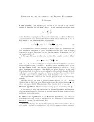
CASO REAL: DOBLE ROTOR
L h , ω h
L v , ω v
Y
X
Z

CASO REAL: DOBLE ROTOR
1) AplicaciA
plicación n de control monovariable.
Se controla el ángulo de asiento (variable controlada) con la tensión al motor principal (variable manipulada):
- manteniendo bloqueado el eje vertical o
- considerando que la tensión al motor de cola actúa como variable de perturbación.
Modelo:
( θ)
( ) ( )
G(s) o
= a s 3 2
3
+ a s a θ s a θ
2
+
1
+
o
b
θ = ángulo de asiento que depende del punto de operación.
140
120
100
b 0
80
60
40
20
0
-45 -40 -35 -30 -25 -20 -15 -10 -5 0
θ

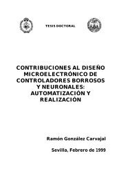
CASO REAL: DOBLE ROTOR
a 1
a1
2.55
2.5
2.45
2.4
2.35
2.3
2.25
2.2
2.15
2.1
2.05
-45 -40 -35 -30 -25 -20 -15 -10 -5 0
θ
a 0
1.75
1.7
1.65
1.6
1.55
1.5
1.45
1.4
1.35
-45 -40 -35 -30 -25 -20 -15 -10 -5 0
θ
o
Modelo de incertidumbre: intervalo de plantas
( ) ∈[ ]
b θ 18.427, 137.9447
o
( ) ∈ [ ] a1( θ) ∈[ 2.0535, 2.5423]
a θ 1.3993, 1.7407
a2
= 1,0711 a3
= 1,4320
1
C(s) = K+ primer orden 16 p. virtuales, diseño o no conservador.
Ts
i

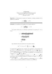
CASO REAL: DOBLE ROTOR
Planta con numerador de grado cero 8 plantas virtuales. . Solución.
k
0.01
0.005
0
Asín
k
-0.006
-0.007
-0.008
-0.009
-0.005
-0.01
-0.015
-0.02
-0.025
-0.01
-0.011
-0.012
-0.013
-0.014
-0.015
-0.016
Zona de estabilidad
Zona de estabilidad
-0.03
-5 0 5 10 15 20
Ti
x 10 4
-3 -2 -1 0 1 2 3 4
x 10 4
Ti
7 polinomios estables, y uno inestable.

CASO REAL: DOBLE ROTOR
Posible modelo conservador:
Conocimiento de la planta relación n lineal entre a 0 y a 1 .
Aproximación politópica
pica de b 0 .
Por ejemplo, si:
los ocho polinomios.
o
( ) ∈[ ]
b θ 18.427, 117.9447
k
se estabilizan
Observaciones:
1) k negativo pequeño
-0.0105
-0.011
2) Ti grande
3) Comportamiento ???
-0.0115
-0.012
Zona de estabilidad
-0.0125
-6000 -4000 -2000 0 2000 4000 6000 8000 10000 12000
Ti

CASO REAL: DOBLE ROTOR
Un parámetro más: m
PID académico:
Diseño o conservador: 32 p. v. (16)
K
= + s P I D
s
I
C(s) K
P+ K
D
, K,K,K > 0
Diseño o no conservador (8 vértices v
+ aristas)
2.5
2
kd=2;
1.5
Zona de estabilidad
de los 8 vértices
kp
1
0.5
0
-0.5
-40 -20 0 20 40 60 80 100
ki

CASO REAL: DOBLE ROTOR
Aristas: casi toda la zona estabiliza las aristas.
1)
KD = 2;K
P=1;KI
= 5;
800
Conjunto de valores
600
400
200
0
-200
-400
-12000 -10000 -8000 -6000 -4000 -2000 0 2000 4000

CASO REAL: DOBLE ROTOR
60
69.75
40
20
0
-20
69.7
69.65
69.6
-40
69.55
-60
69.5
-800 -600 -400 -200 0 200 400 600 800 1000
618.5 619 619.5 620 620.5 621 621.5 622
2)
3)
KD = 2;K
P=1.4;KI
= 0.1;
KD = 2; K
P=0.01; KI
= 2.5;

CASO REAL: DOBLE ROTOR
Comportamiento: D-estabilidad.
El intervalo de plantas puede convertirse en politopo:
‣ Conservador en el modelo
‣ Conservador en el diseño o (menor coste computacional)
Control multivariable: : más m s parámetros, más m s grado de los polinomios
característicos.

OTROS ÁMBITOS
Control Predictivo – politopos de plantas.
Resultados de análisis:
GPC δ(s) es un politopo de polinomios, aplicación RPE
Mean level, Dead beat
CRHPC menos robusto que GPC
Influencia del polinomio T en δ(s)
Dinámicas rápidas r
y lentas: Generalización n del Teorema de
Kharitonov intervalos de polinomios que pueden disminuir de grado.

REFERENCIAS
• Ackermann J., in co-operation with Barlett A., Kaesbauer B., Sienel W., Steinhauser R., “Robust
Control. System with Uncertain Physical Parameters”, , Springer-Verlag, 1993.
• Barmish B.R., “New tools for Robustness of Linear Systems”, , Macmillan Publishing Company.
1993.
• Ghosh B.K., “Some New Results on the Simultaneous Stabilizability of a Family of Single Input,
Single Output Systems”, , Systems and Control Letters, vol. 6, pp. 39-45, 1985.
• Chapellat H., Bhattacharyya S.P., ”A A Generalization of Kharitonov’s s Theorem: Robust Stability
of Interval Plants”, , IEEE Transations on Automatic Control, vol. AC-34, # 3, pp. 306-311, 1989.
• Hollot C.V., Yang F., ” Robust Stabilization of Interval Plants using Lead or Lag Compensators”,
Systems and Control Letters, 14, pp. 9-12, 1990; Proc. of IEEE Conference on Decision and
Control, Diciembre 1989, Tampa, Fl, 1990.
• Barmish B.R., Hollot C.V., Kraus J.F., Tempo R., “Extreme Point Results for Robust
Stabilization of Interval Plants with First Order Compensators”, , IEEE Transactions on
Automatic Control, vol. AC 37, pp.707-714.
• Djaferis T.E., “To Stabilize an Interval Plant Family it Suffices to Simultaneously Stabilize Sixty-
four Polynomials”, , IEEE Transactions on Automatic Control, vol. 38, # 5, pp. 760-764, 1993.

REFERENCIAS
• Hernández
ndez et al., 1995. “On the Sixty-four Polynomials of Djaferis to Stabilize an Interval Plant”,
IEEE Transactions on Automatic Control, Diciembre 1995
• Hernández
ndez et al., 1996. “Comparison between the Thirty-two Virtual Vertices and the Ghosh
Polynomials to Stabilize an Interval plant”, 13 th Triennial World Congress, San Francisco, IFAC
1996
• Hernández
ndez et al., 1998. “ On the Thirty-two Virtual Polynomials to Stabilize an Interval Plant”,
IEEE Transactions on Automatic Control, Octubre 1998
• Hernández
ndez et al., , 1999. “Comparison between the Extreme Point Results to Stabilize an Interval
Plant”, 14 th Triennial World Congress, Beijing, IFAC 1999
• “Kharitonov´s Theorem Extension to Interval Polynomials Which Can Drop in Degree: A
Nyquist approach”, IEEE Transactions on Automatic Control, Diciembre 1995
Hernández R, Dormido S., “Kharitonov’s Theorem Extension for Interval Polynomials which
Can Drop in Degree: A Nyquist Approach”, IEEE Transactions on Automatic Control, vol. 41, #
7, pp. 1-4, Julio 1996.