Introduction au calcul scientifique pour les EDP de la ... - Inria

More documents

Recommendations

Info

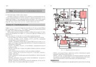
La mise en équationLoi de conservation : ∂θ + div ⃗q = 0.∂tLoi de conduction : ⃗q = −σ∇θ.Si on élimine ⃗q le problème à résoudre s’écrit:⎧Trouver θ(x, t) : Ω×]0, T [−→ R tel que:∂θ⎪⎨ ∂t − div( σ∇θ) = 0, x ∈ Ω, t > 0,σ ∂θ∂n = q l, (−⃗q · n = q l ) x ∈ Γ 1 , t > 0,θ = θ l , x ∈ Γ 0 , t > 0,⎪⎩θ(x, 0) = θ 0 (x), x ∈ Ω.Nature du problème⎧Trouver θ(x, t) : Ω×]0, T [−→ R tel que:∂θ⎪⎨ ∂t − div( σ∇θ) = 0, x ∈ Ω, t > 0,σ ∂θ∂n = q l, x ∈ Γ 1 , t > 0,θ = θ l , x ∈ Γ 0 , t > 0,⎪⎩θ(x, 0) = θ 0 (x), x ∈ Ω.Le temps faisant partie explicitement des variables duproblème, on a affaire à un problème d’évolution.Tant mathématiquement que numériquement,les variables x et t jouent un rôle différent.Introduction au calcul scientifique pour les EDP de la physique. – p.5/27Introduction au calcul scientifique pour les EDP de la physique. – p.6/27Nature du problème⎧Trouver θ(x, t) : Ω×]0, T [−→ R tel que:∂θ⎪⎨ ∂t − div( σ∇θ) = 0, x ∈ Ω, t > 0,σ ∂θ∂n = q l, x ∈ Γ 1 , t > 0,θ = θ l , x ∈ Γ 0 , t > 0,⎪⎩θ(x, 0) = θ 0 (x), x ∈ Ω.L’équation de la chaleur est le prototype des équationsparaboliques qui modélisent les phénomènes de diffusion.Elles interviennent aussi en mécanique des fluides (milieuxporeux, diffusion de polluants), ou en finance (Black-Scholes).Ces équations seront abordées au cours 8.Les difficultés de l’analyse mathématique.Vu de très loin, le problème peut être mis sous la forme:Trouver u ∈ V tel que A u = doù V est un espace vectoriel (espace de fonctions), A est unopérateur linéaire, le vecteur u est la fonction inconnue θ et dreprésente les données (θ 0 , θ l , q l ).Cela ressemble à un système linéaire.Les différences majeures, sources de difficultés, sont:L’espace fonctionnel V est de dimension infinie.L’opérateur A est un opérateur différentiel (non continudans des topologies classiques).De ce fait, les questions d’existence et d’unicité de la solutionsont très délicates.Introduction au calcul scientifique pour les EDP de la physique. – p.6/27Introduction au calcul scientifique pour les EDP de la physique. – p.7/27
Notion de problème bien posé.Notion de problème bien posé.Soit (S, ‖ · ‖ S ) et (D, ‖ · ‖ D ) deux espaces vectoriels normés etF une application (non nécessairement linéaire) de S dans Douvert de D. On dira que le problème:(P ) Trouver u ∈ S tel que F (u) = dest bien posé au sens de Hadamard si:Pour tout d dans D, (P ) admet une solution et une seule.Cette solution dépend continument de la donnée d:d n → d dans D =⇒ u n → u dans SAttention, la notion de problème bien posé n’est pasintrinsèque. Elle est liée au choix des espaces S et Det surtout au choix des normes ‖ · ‖ S et ‖ · ‖ D .On dit aussi que le problème est stable en norme ‖ · ‖ Spar rapport à la norme ‖ · ‖ D .La notion de stabilité du problème continu est un pré-requisquasiment indispensable en vue de l’approximation numérique.Dans le cas F linéaire , D = D et la condition de continuité setraduit par l’existence d’une constante C telle que:‖u‖ S ≤ C ‖d‖ D .Introduction au calcul scientifique pour les EDP de la physique. – p.8/27Introduction au calcul scientifique pour les EDP de la physique. – p.9/27Stabilité L 2 du problème de Cauchy.L’estimation a priori.On admet ici le résultat d’existence et unicité pour notreproblème modèle et on va s’intéresser à un résultat de stabilité.On va se restreindre à θ l = q l = 0 auquel cas la seule donnéeest θ 0 (problème de Cauchy).On va établir le résultat de stabilité:∀ t > 0,‖θ(t)‖ L 2 (Ω) ≤ ‖θ 0 ‖ L 2 (Ω).Le résultat va apparaître comme une estimation a priori, c’est àdire une estimation qu’on est capable d’obtenir sans connaîtreexplicitement la solution.Introduction au calcul scientifique pour les EDP de la physique. – p.10/27On multiplie l’équation par θ et on intègre sur Ω:∫∂θΩ ∂t∫Ωθ dx − div ( σ∇θ) θ dx = 0On remarque que:∫Ω∂θ∂t θ dx = ∫Ω∂∂t( θ2 )dx = 1 ∫d2 2 dtΩθ 2 dx.On utilise la formule de Green (intégration par parties):∫− div ( ∫∫σ∇θ) θ dx = σ|∇θ| 2 ∂θdx − σ∂n θ dγΩ(θ s’annule sur Γ 0 , ∂θ∂n sur Γ 1.)ΩΓIntroduction au calcul scientifique pour les EDP de la physique. – p.11/27
Page 4 and 5: L’estimation a priori.L’estimat
Page 6 and 7: Construction d’opérateurs aux di
Page 9 and 10: L’analyse numérique.C’est une

Introduction au calcul scientifique pour les EDP de la ... - Inria

You also want an ePaper? Increase the reach of your titles

Delete template?

Save as template?