Diameter of Opportunistic Mobile Networks - Paris Research ...

3.1.2 Continuous-time modelIn the discrete-time model above, for any pair ofnodes (u, v) the set of indices t such that edge (u, v)is in E t is a sequence of integers in N separated by geometricrandom variables. A natural generalization ofthe model to a continuous time setting is then to assumethat, for any pairs of nodes (u, v), the times ofcontact are separated by exponential random variables.In other words, this process of time instants constitutesa Poisson process.A random temporal network (in continuous time) is aprocess of graphs { G t = (V, E t ) | t ∈ R + } such that:• N (u,v) = { t | (u, v) ∈ E t } is a Poisson processwith rate λ/(N − 1).• Processes in the collection { N (u,v) | (u, v) } aremutually independent.This model may use either directed or undirected edges.3.1.3 Paths in long contact case/short contact caseA path from u to v in a temporal network is a sequenceu = u 0 ❀ t1 u 1 ❀ · · · ❀ t ku k = v such that:(i) (u i−1 , u i ) ∈ E ti for all i = 1, . . .,k,(ii) t i+1 ≥ t i for all i = 1, . . . , k.We assume that all contacts have a fixed durationthat is either one time slot (in the discrete time model)or negligible (in the continuous time model). To modelthe impact of a limited local bandwidth, or local latency,on the properties of paths, we introduce two cases.We define the long contact case as the model whereany number of edges may be used in a single time slot, asallowed by the definition of a path found above. In otherwords we assume that a single time slot is sufficientlylong to exchange across several contacts.On the contrary, we define the short contact case asthe model where only one contact may be used in asingle time slot. In other words, we require that allpaths verify, in addition to the conditions above:(ii ′ ) t i+1 ≥ t i + 1 for all i = 1, . . . , k.3.2 Phase transitionIn this section, we first prove a result on the expectednumber of paths between two nodes, when delay andhops are constrained. This result is then used to describea phase transition for the appearance of paths ina random temporal network.3.2.1 Expected number of paths with constraintsWe describe now our main analytical results, whichcharacterize the expected number of paths with constraintson both delay and hop-number. A source uand a destination v are fixed in advance and withoutloss of generality we assume that the packet is ready tobe sent at the source at time t = 0.Since we are interested in large networks, with a constantcontact rate per node, we let N go to infinity andlimit the time and the number of hops allowed in thepaths by a slowly increasing function of N.Lemma 1. Let us denote the maximum time t N andmaximum hops k N of a path allowed in the network.We assume that they are given as a function of N by:{tN = τ · ln(N),(1)k N = γ · t N = γ · τ · ln(N),where τ and γ are two positive constants.Let us denote by Π N the number of paths from u tov under the above constraints. Then, as N grows large- for short contacts, E[Π N ] = Θ−1+τ(γ(Nln(λ)+h(γ)))where h : x ∈ [0; 1] ↦→ −xln(x) − (1 − x)ln(1 − x).- for long contacts, E[Π N ] = Θ−1+τ(γ(Nln(λ)+g(γ)))where g : x ∈ [0; 1] ↦→ (1 + x)ln(1 + x) − xln(x).Proof. This proof follows from the memoryless propertyof geometric and exponential distributions. Wefirst estimate the probability of success of a path whosenodes are fixed in advance. The expectation is thenthis probability multiplied by the number of possiblecombinations. Stirling formula is used to complete theargument. It can be found in [12].We have, as a direct consequence of Lemma 1.Corollary 1. Under the assumption above we have,in the short contact case{E[ΠN ] → 0 if 1/τ > γ ln(λ) + h(γ)E[Π N ] → ∞ if 1/τ < γ ln(λ) + h(γ).The first result implies that, when 1/τ > γ ln(λ)+h(γ):P [ There exists a path with constraints (1) ] → 0All these results holds for the long contact case whenreplacing the function h by g.Proof. The first results follows directly from theproperties of the expectation found above. The lastresult is a consequence from the Markov inequality:P [Π N ≥ 1] ≤ E[Π N ] .3.2.2 Phase transition in the short contact caseThe results from the previous section prove that, dependingon the values of the two constant numbers τand γ, as well as the contact rate λ, one of the two followingstatements holds: either there almost surely doesnot exist a path satisfying the logarithmic bound (1); orthe number of paths that satisfy these conditions growson average to infinity with N. Moreover, one can tell3

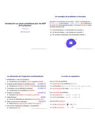
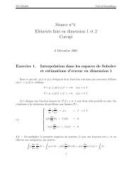
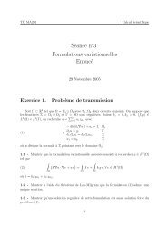
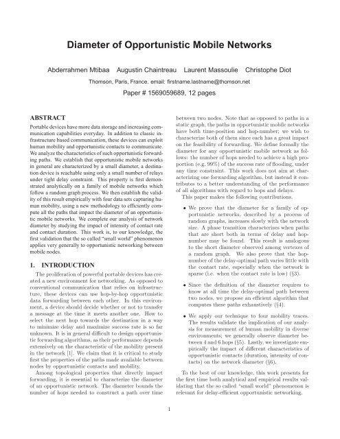
γ ln(λ) +h(γ)1.210.80.60.40.200λ = 1.5λ = 1.0λ = 0.50.2M = ln(1 + λ)γ = λ1+λ0.4γ0.60.8Figure 1: Phase transition (short contact case)which statement holds simply by comparing the valuesof 1/τ and γ ln(λ) + h(γ).This result might be interpreted as follows. Note thatthe short contact case implies γ ≤ 1. The functionγ ∈ [0; 1] ↦→ γ ln(λ) + h(γ) admits a maximum, that isgiven by M = ln(λ + 1) and this maximum is attainedwhen γ = λ1+λ. This is illustrated on Figure 1 where thevalue of this function of γ was plotted for three differentvalues of λ. We can deduce the following dichotomy:• If τ < 1/M = 1/ ln(1 + λ), then 1/τ is alwayslarger than γ ln(λ) + h(γ) for any value of γ. As aconsequence, almost surely there does not exist apath with delay less τ ln(N) when N is large.• If τ > 1/ ln(1+λ), then the super-critical conditionfrom Corollary 1 is verified for γ ∈ [γ 1 ; γ 2 ], anλinterval which contains1+λ. As a consequence,the average number of paths with delay τ ln(N)and γτ ln(N) hops is unbounded for large N,The delay-optimal path corresponds to the criticalvalue of τ for which a path is likely to be found. From aheuristic standpoint, we then expect the delay-optimalln(N)ln(1+λ)path to have delay t ≈ . When τ approachesthis critical value, the interval of possible values for γbecomes small, and centered around λ1+λ. Hence, we expectthat the delay optimal path has hop-number givenλ ln(N)by k ≈(1+λ)·ln(1+λ). As an example, when λ = 0.5, weexpect a delay growing with N as t ≈ 2.47 · ln(N) andwe expect a number of hops k ≈ 1.64 · ln(N).3.2.3 Phase transition in the long contact caseIn the long contact case, the expected number ofpaths with delay and hop constraints, for large N, becomeslarge if 1/τ < γ ln(λ) + g(γ). In contrast with1the short contact case, the properties of this function ofγ change with the value of λ (see Figure 2). As a result,we look at the cases λ < 1 and λ > 1 separately.γ ln(λ) +g(γ)3.532.521.510.5000.5λ = 1.5λ = 1.0λ = 0.5M = − ln(1 − λ)1γγ = λ1−λ1.5Figure 2: Phase transition (long contact case)• When λ < 1, the result is very similar to the shortcontact case. The function of γ admits a maximumM = − ln(1 − λ), attained when γ = λ1−λ .Following the same heuristic as the short contactcase, we expect the delay-optimal path to haveln(N)2λln(N)−(1−λ)·ln(1−λ) hops.delay t ≈−ln(1−λ) and k ≈As an example, when λ = 0.5, we expect a delayt ≈ 1.69 · ln(N) and the same number of hops.• When λ > 1, we notice a difference with the shortcontact case, since the function of γ is increasingand unbounded. In that case, for any τ, even anarbitrary small constant, some paths exist with adelay less than τ ln(N).To compute the hop-numbers of these paths, weproceed as follows. Since 1/τ is large, γ shouldthen be sufficiently large to satisfy the conditionof the corollary. The function of γ is then close toits asymptote γ ↦→ 1+γ ln(λ). We deduce that the1−τsmallest value of γ verifying the condition isτ ln(λ) ,hence k = γτ ln(N) given by k ≈ ln(N)/ln(λ).This last regime should not come as a surprise: in astatic random graph, there exists a phase transitionwhen λ approaches 1. In particular, when λ is greaterthan 1, there almost surely exists a unique connectedcomponent with a large size (see Theorem 5.4 p.109 in[6]). In our model, since the long contact case allowsone to use any number of hops during the same timeslot, this property implies that there does exist pathsfor any arbitrarily small τ. In other words, although4

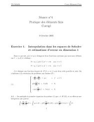
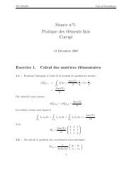
the network is still changing with time, it is essentially“almost-simultaneously connected”.3.3 Impact of the contact rateWe have seen above that the value of the contactrate λ impacts qualitatively the phase transition in thelong contact case, as λ becomes larger than 1. Moregenerally, when λ is less than 1, it has a direct impacton the delay of the paths present in a random temporalnetwork. We note in particular that as λ gets small,the minimum value of τ for which a path may exist(respectively 1/ ln(1+λ) and −1/ ln(1−λ) for the shortand the long contact case) becomes large.In contrast with delay, the hop-number of a pathvaries little as λ changes. In particular, when λ becomessmall, the hop-number for the delay-optimal pathin both short and long contact cases no longer dependson λ and it converges to ln(N).kln(N)5432100.001long-contactshort-contact0.010.1λFigure 3: Hop-number of the delay-optimal pathseen as a function of the contact rateOne may think of the following explanation for thisresult: As λ decreases, the network is essentially completelydisconnected except occasionally for one or severaldisjoint pairs of nodes. Therefore, if we rescale timeby merging periodically a fixed number of time slots together,the network appears to be very similar (a fewdisjoint pairs of nodes) except for an appropriate scalingof the contact rate. As a consequence, decreasingλ linearly increases the time needed to create a path,but is unlikely to impact the actual hop-number of thispath. The analysis above makes this intuition rigorous.We summarize our results in Figure 3. The y-axisrepresents the estimate of the hop-number for the delayoptimalpath, normalized by ln(N). We see that in bothdense and sparse regimes, short and long contacts arein good agreement. They differ only near the critical110value λ = 1, where the long contact case has a singularity.This singularity is not likely to occur in practiceas bandwidth limits the hops in a single time slot.3.4 DiscussionsWe have studied the properties of random temporalnetworks, as they become large. We have shown thata source destination pair admits on average many forwardingpaths using a small number of hops and over ashort number of time-slots (i.e. both grow as the logarithmof the network size). Note that the delay of theoptimal paths depends heavily on the contact rate betweenthe nodes. On the other hand, the hop-numberof these paths seems rather insensitive to changes inthe contact rate λ, with the only exception of the longcontactcase around the value λ = 1.Inspired by these results, one may compute the diameterof a network using the paths with an optimal delay,and deduce that temporal networks generally havea small diameter, for almost any contact rate. However,our model is based on several important simplificationsthat may impact in general the delay and hop-numberof paths in opportunistic networks:• Homogeneity: We have assumed that nodes contactothers uniformly at random. In practice thisis not true as people tend to come close to eachother according to their habits and the communitiesof interest that they share.• Inter-contact time statistics: Since we assumethat contacts between nodes follow Bernoulli orPoisson Processes, the distribution of time betweentwo contacts of a pair is light tailed. Previous experimentshave shown that this assumption holdsonly at the timescale of days and weeks [1, 7].It is nevertheless possible to extend all of the resultswe have obtained so far to contacts describedby a renewal process with general inter-contacttime distribution with finite variance. We expectthis to have a major impact on the delay of a path,but a relatively small impact on hop-number.• Stationarity: This model does not include periodicdiurnal cycles in the variation of the contactrate that are typically found in human mobility.The network may change from a highly mobile anddense subset of contacts into a sparse and slowlyvarying subset of contacts. Again, we expect thiseffect to impact the delay of paths in temporalnetwork, but not much their hop-number.In the rest of this article, after having formally definedthe diameter of any temporal network, we estimate itsvalue for mobility traces where in general none of theseassumptions holds. Our goal is to demonstrate that thefundamental insight brought up by this simple modeltranslate in practice into similar qualitative trends.5

4. NETWORK DIAMETER DEFINITIONAND MEASUREMENT METHODIn this section, we first formalize our definition of networkdiameter. We then describe an algorithm to studyefficiently and exhaustively the properties of delay optimalpaths in opportunistic networks. This algorithmis instrumental to study the diameter found in largetraces, as done in the next section. It is one of thecontributions of this work.4.1 Definition of diameterThe diameter of a network is an upper bound on thenumber of intermediate hops needed to find at leastone path between any two nodes. What is essentiallynew in a temporal network is that one has to specifywhether this path should also satisfy a condition on itstime characteristics. Inspired by the results from theprevious section, we define the diameter such that werequire this path to be almost always optimal.For k ∈ N ∪ {∞}, and t ≥ 0 let Π(t, k) be 1 if thereexists a path that uses at most k hops and succeeds todeliver a packet within t seconds, let Π(t, k) be 0 otherwise.This variable depends on the source, destination,and starting time of the packet. For ε > 0, we definethe (1 − ε)-diameter as the integer k such that∀t ≥ 0 , P [Π(t, k) = 1] ≥ (1 − ε) · P [Π(t, ∞) = 1] ,and k is the minimum number that verifies it.This expression can be interpreted in two ways: in astochastic model of a stationary homogeneous network,like the one we studied in §3, the probability is chosenaccording to the distribution of the random variablesΠ(t, k) seen at any time between any two nodes. In amobility data set, we consider the empirical probabilitycombining uniformly observations for all sources, destinationsand starting times. In both case, this expressionstates that, for any delay-constraint, it is almostas likely to find a successful paths within k hops thanwith any more hops.One may think of this definition as an example of“competitive analysis” since the success ratio (i.e., theprobability to find a path within t seconds and at mostk hops) is not described in absolute term, but insteadis compared with an optimal strategy. It helps the definitionto adapt to variable environments. However,it requires one to know beforehand the performance ofthe delay-optimal paths at all time, which is why weformally describe in the rest of this section how theycan be extracted from traces.4.2 Paths in temporal networksEach data set may be seen as a temporal network.More precisely we represent it as a graph where edgesare all labeled with a time interval, and there may bemultiple edges between two nodes. A vertex representsa device. An edge from device u to device v, with label[t beg ; t end ], represents a contact, where u sees v duringthis time interval. The set of edges of this graph thereforeincludes all the contacts recorded by each device.Paths associated with a sequence of contacts:We intend to characterize and compute in an efficientway all the sequences of contacts that are available totransport a message in the network. Note that we allowsimultaneous contacts to be used, as in the long contactcase defined in §3.1. It is possible to include a positivetransmission delay in all these definitions, we expectthat the diameter will be smaller in that case.A sequence (e i = (v i−1 , v i , [t begi ; t endi ])) i=1,...,n of contactsis valid if it can be associated with a time respectingpath from v 0 to v n . In other words, it isvalid if there exists a non-decreasing sequence of timest 1 ≤ t 2 ≤ . . . ≤ t n such that t begi ≤ t i ≤ t endi for all i.An equivalent condition is given by:∀i = 1, . . .,n, t endi≥ maxj

made with a single contact, but sequences with multiplecontacts, like Figure 4 (a), might not verify EA ≤ LD.∞del(t)EA 4 > LD 4(v 1, v 2)EA 2(v 0, v 1)LD 2EA 2 LD 2EA 1 LD 1(v 0, v 1, v 2)LD EA(a)EA 1 LD 1EA LD(b)EA 3 < LD 3EA 2 = LD 2Figure 4: Two examples of concatenation4.3 Delay-optimal pathsSo far we have been describing a method to characterizewhen a sequence of contacts supports a timerespectingpath, and when we can concatenate them.However, computing all of them in general is very costly.In this section, we formally define paths that are optimalin terms of delay, and therefore are susceptible toimpact the diameter of the network. Later, we focus oncomputing only those paths.Delivery function: As a consequence of (ii) and(iii), for a message created at v 0 at time t, if t ≤ LDthen there exists a path associated with the sequenceof contacts e, that transports this message and deliversit to v n at time max(t,EA). Otherwise, when t > LD,no path based on these contacts exists to transport themessage. The optimal delivery time of a message createdat time t, on a path using this sequence of contacts,is given by{ max(t,EA) if t ≤ LD,del(t) =∞ else.Similarly the optimal delivery time for any paths thatuse one of the sequences of contacts e 1 , . . .,e n is givenby the minimumdel(t)=min{max(t,EA k ),1 ≤ k ≤ n s.t. t ≤ LD k }(3)where, following a usual convention, the minimum of anempty set is taken equal to ∞.Optimal paths: We say that a time respecting path,leaving device v 0 at time t dep , arriving in device v n attime t arr , is strictly dominated in case there exists anotherpath from v 0 to v n with starting and ending timest ′ dep , t′ arr such that (t′ dep ≥ t dep and t ′ arr ≤ t arr), andif at least one of these inequalities is strict. A path issaid optimal if no other path strictly dominates it.According to (ii) and (iii) above, among the paths associatedwith a sequence of contacts with values (LD,EA)the optimal ones are the following: ifLD ≤ EA, this is thepath starting at time LD and arriving at time EA. Otherwise,when LD > EA, all paths that start and arrive atthe message generation time t ∈ [EA;LD] are optimal.EA 1 < LD 1LD 1LD 2LD 3LD 4time tFigure 5: Example of a delivery function, andthe corresponding pairs of values (LD i ,EA i ) i=1,2,3,4 .An example of delivery function is shown in Figure 5.Note that the value of the delivery function (y-axis) maybe infinite. Pairs (LD 1 ,EA 1 ) to (LD 3 ,EA 3 ) satisfy EA ≤LD, they may correspond to direct source-destinationcontacts, or sequence of contacts that all intersect atsome time; the fourth pair verifies LD 4 < EA 4 , hence itdoes not correspond to a contemporaneous connectivity.The message needs to leave the source before LD 4 , andremains for sometime in an intermediate device beforebeing delivered later at time EA 4 .4.4 Efficient computation of optimal pathsWe construct the set of optimal paths, and deliveryfunction for all source-destination pairs, as an inductionon the set of contacts in the traces. We representthe delivery function for a given source-destination pairby a list of pairs of value (LD,EA). The key element inthe computation is that only a subset of these pairs isneeded to characterize the function del. This subsetcorresponds to the number of discontinuities of the deliveryfunction, and the number of optimal paths thatcan be constructed with different contact sequences.We use the following observation: We assume thatthe values (LD k ,EA k ) k=1,...,n , used to compute the deliveryfunction as in (3), are increasing in their firstcoordinate. Then, as k = n, n − 1, . . ., we note that thek th pair can always be removed, leaving the functiondel unchanged, unless this pair verifies:EA k = min { EA l | l ≥ k } . (4)In other words, a list such that all pairs verify this conditiondescribes all optimal paths, and the functiondel,using a minimum amount of information.As a new contact is added to the graph, new sequencesof contacts can be constructed thanks to theconcatenation rule (fact (iv) shown above). This createsa new set of values (LD,EA) to include in the list7

of different source-destination pairs. This inclusion canbe done so that only the values corresponding to anoptimal path are kept, following condition (4).We show that our method can also be used to identifyall paths that are optimal inside certain classes, forinstance the class of paths with at most k hops. Thiscan be done by computing all the optimal paths associatedwith sequences of at most k contacts, starting withk = 1, and using concatenation with edges on the rightto deduce the next step.Compared with previous generalized Dijkstra’s algorithm[5], this algorithm computes directly representationof paths for all starting times. That is essentialto have an exhaustive search for paths, and estimatethe diameter of a network at any time-scale. We foundalgorithm UW2 in [14] to be the closest to ours. Wehave introduced here an original specification througha concise representation of optimal paths which makesit feasible to analyze long traces with hundred thousandsof contacts. Recently we have found that anotheralgorithm has been developed independently to studyminimum delay in DTN [18]. It works as follows: apacket is created for any beginning and end of contacts;a discrete event simulator is used to simulate flooding;the results are then merged using linear extrapolation.5. EMPIRICAL RESULTSIn this section we present first our data sets. Thenwe analyze the characteristics of optimal paths in opportunisticnetworks using the methodology describedin the previous section.5.1 Mobility data setsWe use four experimental data sets. Three have beencollected by the Haggle Project [1]. They include twoexperiments conducted during conferences, Infocom05,Infocom06, and one experiment conducted in Hong-Kong.The fourth data set has been collected by the MIT RealityMining Project [2]. Table 1 summarizes importantcharacteristics of these data sets.In the Haggle experiments, people were asked to carryan experimental device (i.e., an iMote) with them at alltimes. These devices log all contacts between experimentaldevices (i.e., called here internal contacts) usinga periodic scanning every t seconds, where t is calledgranularity. In addition, they log contacts with otherexternal Bluetooth devices (i.e., external contacts) thatthey meet opportunistically (e.g., cell phones, PDAs,laptops).In Infocom05, Infocom06 the experimental deviceswere distributed to students attending the conferencefor several consecutive days. The largest experiment isInfocom06 with 78 participants. By default we are presentinghere results for internal contacts only; resultswith internal and external contacts are very similar.In Hong-Kong, people carrying the experimental deviceswere chosen carefully in a Hong Kong bar to avoidsocial relationships between them. These people returnedthe iMote at the same bar a week later. As aconsequence, there are only few internal contacts, whichis why we are presenting here results with both internaland external contacts.Note that we may not collect all opportunistic encountersbetween participants of the experiment, becauseof the time between two scans, hardware limitations,software parameters, and interference [13]. Forthe same reasons, it is also possible that some contactsappear shorter than they are. In addition, we do nothave access to the contact history of the external devicesand, as consequence, we miss some of the directcontacts between them as well. We examine the impactof this “sampling” effect in §6.The Reality Mining data set includes records fromBluetooth contacts and GSM base stations for a groupof cell-phones distributed to 100 MIT students during 9months. We only show results from the Bluetooth dataset. We also made the same observations on the GSMdata set, as well as other publicly available data sets,including traces from campus WLAN in Dartmouth [4]and UCSD [11].5.2 Preliminary observationsFigure 6 shows the sequence of contacts with anyother device in the course of the experiment (for sixrepresentative participants (y-axis) of Infocom05). Thenext time the device will be in range of any other device(z-axis) is plotted as a function of time (x-axis). Thediagonal represents a period of uninterrupted contact.The steps correspond to period with no contact at all.Time of Next Contactinf12am12am12am12amnode 36403435393712amFigure 6: Time to contact any other device, forsix participants during Infocom05.Extended periods of high connectivity, where the deviceis always in reach of one or several devices alternate12amTime12am8

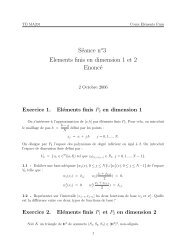
Experimental data set Infocom05 Infocom06 Hong-Kong Reality Mining BTDuration (days) 3 4 5 246Granularity (seconds) 120 120 120 300Number of experimental Devices 41 78 37 100Number of internal Contacts 22,459 182,951 560 54,667Rate of contact (only internal contacts) 1.10 1.70 8.6 ×10 −3 15 ×10 −3Number of external Devices 223 4,649 831 N/ANumber of external Contacts 1,173 11,630 2,507 N/ARate of contact (incl. external contacts) 1.39 2.53 98 ×10 −3 N/ATable 1: Characteristics of the four experimental data setswith periods of complete disconnection that are mostoften corresponding to night time.10.1Reality MiningHong KongInfocom05Infocom06pair in Hong Kong, the delivery function when pathswith different number of hops (i.e. intermediate relays)are used.Arrival Timeinf12amCCDF0.0112am12am12am0.00112am1e-041min 2min 10min1hour 3h 12hContact durationFigure 7: Distribution of contact duration12amsingle hophops = 234inf12am12am12am12am12amDeparture Time12amFigure 7 plots distributions of contact duration forthe four data sets. This figure shows that contact durationvary a lot in all traces (from a couple of minutes upto several hours). Above 75% of contacts (143,502 contacts)in Infocom06 are only one slot long (i.e. 2 minutes).This can be partly explained by the samplingeffect mentioned in §5.1. However we still find around0.4% (765 contacts) that are longer than one hour. Thishas two important consequences: First, a path computationtechnique should be able to handle contacts ofdifferent sizes represented as intervals of times, ratherthan relying on a discrete time representation of thedata set. Second, one should consider whether contactsthat are short are actually useful to carry data, andwhat are the implications of this limitation. We discussthese points further in §6.2.5.3 Properties of Delay-optimal PathsFollowing the methodology described earlier, we computethe sequence of optimal paths found between anysource and destination in the network, varying the maximumnumber of hops in a path between 1 and 4, andinfinity. Figure 8 shows, for a given source-destinationFigure 8: Example of a delivery function, fora given source-destination pair during Hong-Kong, for paths with various number of hops.In the example shown here, there is no path from thesource to the destination when using paths with lessthan 3 hops. When 4 hops can be used, the number ofoptimal paths increases to 5. We see on this figure thatthere is no optimal path with more than 4 hops, as thedelivery function is identical when the maximum hop isset to four or infinity. Similar results were obtained forInfocom05 and can be found in [12].5.3.1 Distribution of delayFrom the sequence of delay-optimal paths we deducethe delay obtained by the optimal path at all time. Wecombine all the observations of a trace uniformly amongall sources, destinations, and for every starting time (inseconds). We present this aggregated sample of observationsvia its empirical CDF in Figure 9, where themaximum hop-number varies between 1, 4 or 6, and infinity.Note that the value of the CDF for a given timet is equal to the probability to successfully find a path9

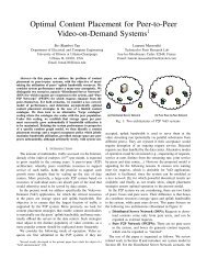
1110.10.10.1P[Delay < D ]0.01P[Delay < D ]0.01P[Delay < D ]0.010.001unlimited hops5 hops4 hops3 hops2 hopssingle hop0.001unlimited hops5 hops4 hops3 hops2 hopssingle hop0.001unlimited hops5 hops4 hops3 hops2 hopssingle hop2 min10 min1 hour 3 h 6 h1 day2 min 10 min1 hour 3 h 6 h 1 day2 min 10 min1 hour 3 h 6 hDelay DDelay DDelay D(a) Original data set(b) 10% of contacts remaining(c) 1% of contacts remainingFigure 10: Empirical CDF of minimum delay when contacts are removed randomly (Infocom06)diameter of the network, which remains under 5 hops.Moreover, as contacts are removed the improvement introducedby using several intermediate hops becomesless important at small time-scale, and remains importantat large time-scale. This confirms the intuitionthat improvement at small time scales is related to highcontact rate values (as seen in §5.3.1).observe that the diameter decreases with delay for highcontact rate. In contrast, the diameter increases withdelay when the contact rate is low. In between, we findan intermediate regime where the diameter might belarger for a narrow range of time. We conjecture this isbecause the network remains connected but lacks shortcutsbetween far-away nodes.6.2 Contact durationWe now remove each contact if it lasts less than t seconds,where t is a fixed threshold. Figure 11 presentsthe empirical CDF of the minimal delay after we removecontacts that last less than 2, 10 and 30 minutes(respectively 75%, 92% and 99% of contacts removed).Contacts that are less than 2 minutes are those with adevice seen during a single scan. When these contactsare removed, the success probability is divided by twoat any time scale, but all the results we have obtainedremain.Interestingly the diameter changes when we only keepcontacts that last more than 10 minutes. First notethat the probability to find a path with delay less than10 minutes remains above 5%, while it was 2% when wehad removed 90% of contacts randomly. In other words,keeping only the longest contacts maintain more availablepaths within a small delay. However this comes atthe cost of an increased diameter.One explanation for this phenomenon is that contactsare with different types: long contacts with less mobilenodes, or familiar people, and short contact where peopleare met that are belonging to any other part of thegroup. This result suggests that opportunistic schemeshave to take advantage of short contacts (less than 10minutes), not only because there are many, but alsobecause those may help to keep the diameter small.As a summary, Figure 12 plots the diameter (withconfidence level 99%) for each delay separately. As suggestedbefore by a comparison between data sets, we7. CONCLUSIONThis work establishes the existence of the so-called“small-world” phenomenon in opportunistic mobile networks.In particular, we have shown both analyticallyand empirically that the network diameter, that we defineas a general bound on the number of hops neededto successfully transmit a message under constraineddelay, is generally small compared to the number ofdevices in the network. From a theoretical perspective,we have proved that the diameter grows slowly with thenetwork size in a simple random case. We have also analyzedmultiple human contact traces and observed thatthe network diameter generally varies between 3 and6 hops, for networks containing from 40 up to a hundredof nodes. This result holds for sparse and densenetworks, and the diameter varies only a little whencontacts are removed.This result has important impacts on how to designforwarding algorithms in opportunistic networks. Inparticular, it indicates that messages can be discardedafter a few number of hops without occurring more thana marginal performance cost.We now describe some important future extensionsfor this work. First, note that Corollary 1 proves thatthe expected number of paths becomes large under supercriticalcondition, but it does not prove that a pathexist almost surely. Proving this last result is more difficult,and beyond the scope of this paper as the classicalconcentration method known as “second moment”(e.g. p.54 in [6]) does not apply. Second, this paper11

1110.10.10.1P[Delay < D ]P[Delay < D ]P[Delay < D ]0.010.010.010.0012 min10 min1 hourunlimited hops5 hops4 hops3 hops2 hopssingle hop3 h6 h1 day0.0012 min10 min1 hourunlimited hops7 hops5 hops4 hops3 hops2 hopssingle hop3 h6 h1 day0.0012 min10 min1 hourunlimited hops5 hops4 hops3 hops2 hopssingle hop3 h6 hDelay DDelay DDelay D(a) contact durations > 2mn(b) contact durations > 10mn(c) contact durations > 30mnFigure 11: Empirical CDF of minimum delay when short contacts are removed (Infocom06)Hops needed (sucess rate > 99%flooding)7654321010min1hourDelay DInfocom06Contacts>10mnContacts>30mnFigure 12: Diameter as a function of delayproves that short paths generally exist between any twonodes, but it does not indicate whether these paths canbe found efficiently by a distributed algorithm usinglocal information in the nodes. This topic has been addressedon static graphs with a more complex model [9],but the extension of these results to temporal networksremains an open problem. Third, we wish to study theimpact of the heterogeneity of contact rates among thenodes.8. REFERENCES[1] A. Chaintreau, P. Hui, J. Crowcroft, C. Diot, J. Scott, andR. Gass. Impact of human mobility on opportunisticforwarding algorithms. IEEE Trans. Mob. Comp.,6(6):606–620, 2007.[2] N. Eagle and A. Pentland. Reality mining: Sensingcomplex social systems. Journal of Personal andUbiquitous Computing, 10(4):255–268, 2005.[3] M. Grossglauser and D. Tse. Mobility increases thecapacity of ad hoc wireless networks. IEEE/ACM Trans.on Net., 10(4):477–486, 2002.[4] T. Henderson, D. Kotz, and I. Abyzov. The changingusage of a mature campus-wide wireless network. In3h12hProceedings of ACM MobiCom, 2004.[5] S. Jain, K. Fall, and R. Patra. Routing in a delay tolerantnetwork. In Proceedings of ACM SIGCOMM, 2004.[6] S. Janson, T. ̷Luczak, and A. Ruciński. Random Graphs.John Wiley & Sons, 2000.[7] T. Karagiannis, J.-Y. Le Boudec, and M. Vojnovic. Powerlaw and exponential decay of inter contact times betweenmobile devices. Technical Report MSR-TR-2007-24,Microsoft Research Cambridge, 2007.[8] D. Kempe, J. Kleinberg, and A. Kumar. Connectivity andinference problems for temporal networks. In Proceedingsof ACM STOC, 2000.[9] J. Kleinberg. The small-world phenomenon: Analgorithmic perspective. 2000.[10] J. Leskovec, J. Kleinberg, and C. Faloutsos. Graphs overtime: densification laws, shrinking diameters and possibleexplanations. In Proceeding of ACM SIGKDD, 2005.[11] M. McNett and G.M. Voelker. Access and mobility ofwireless PDA users. SIGMOBILE Mob. Comput.Commun. Rev., 7(4):55–57, 2003.[12] A. Mtibaa, A. Chaintreau, L. Massoulié, and C. Diot. Thediameter of opportunistic mobile networks. TechnicalReport CR-PRL-2007-07-0001, Thomson, 2007.available online at http://www.thlab.net[13] E. Nordström, C. Diot, R. Gass, and P. Gunningberg.Experiences from measuring human mobility usingbluetooth inquiring devices. In Proceedings of WorkshopACM MobiEval, 2007.[14] A. Orda and R. Rom. Shortest-path and minimum-delayalgorithms in networks with time-dependent edge-length.J. ACM, 37(3):607–625, 1990.[15] M. Papadopouli and H. Schulzrinne. Seven degrees ofseparation in mobile ad hoc networks. In Proceedings ofIEEE GLOBECOM, 2000.[16] V. Srinivasan, M. Motani, and W. Tsang Ooi. Analysisand implications of student contact patterns derived fromcampus schedules. In Proceedings of ACM MobiCom, 2006.[17] J. Su, A. Goel, and E. de Lara. An empirical evaluation ofthe student-net delay tolerant network. In Proceedings ofIEEE Mobiquitous, 2006.[18] X. Zhang, J. Kurose, B. N. Levine, D. Towsley, andH. Zhang. Study of a bus-based disruption tolerantnetwork: Mobility modeling and impact on routing.Technical Report 07-12, UMass CMPSCI, 2007.[19] W. Zhao, M. Ammar, and E. Zegura. A message ferryingapproach for data delivery in sparse mobile ad hocnetworks. In Proceedings of ACM MobiHoc, 2004.12