Introduction au calcul scientifique pour les EDP de la ... - Inria
Introduction au calcul scientifique pour les EDP de la ... - Inria
Introduction au calcul scientifique pour les EDP de la ... - Inria
- No tags were found...

You also want an ePaper? Increase the reach of your titles
YUMPU automatically turns print PDFs into web optimized ePapers that Google loves.
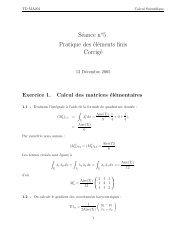
La mise en équationLoi <strong>de</strong> conservation : ∂θ + div ⃗q = 0.∂tLoi <strong>de</strong> conduction : ⃗q = −σ∇θ.Si on élimine ⃗q le problème à résoudre s’écrit:⎧Trouver θ(x, t) : Ω×]0, T [−→ R tel que:∂θ⎪⎨ ∂t − div( σ∇θ) = 0, x ∈ Ω, t > 0,σ ∂θ∂n = q l, (−⃗q · n = q l ) x ∈ Γ 1 , t > 0,θ = θ l , x ∈ Γ 0 , t > 0,⎪⎩θ(x, 0) = θ 0 (x), x ∈ Ω.Nature du problème⎧Trouver θ(x, t) : Ω×]0, T [−→ R tel que:∂θ⎪⎨ ∂t − div( σ∇θ) = 0, x ∈ Ω, t > 0,σ ∂θ∂n = q l, x ∈ Γ 1 , t > 0,θ = θ l , x ∈ Γ 0 , t > 0,⎪⎩θ(x, 0) = θ 0 (x), x ∈ Ω.Le temps faisant partie explicitement <strong>de</strong>s variab<strong>les</strong> duproblème, on a affaire à un problème d’évolution.Tant mathématiquement que numériquement,<strong>les</strong> variab<strong>les</strong> x et t jouent un rôle différent.<strong>Introduction</strong> <strong>au</strong> <strong>calcul</strong> <strong>scientifique</strong> <strong>pour</strong> <strong>les</strong> <strong>EDP</strong> <strong>de</strong> <strong>la</strong> physique. – p.5/27<strong>Introduction</strong> <strong>au</strong> <strong>calcul</strong> <strong>scientifique</strong> <strong>pour</strong> <strong>les</strong> <strong>EDP</strong> <strong>de</strong> <strong>la</strong> physique. – p.6/27Nature du problème⎧Trouver θ(x, t) : Ω×]0, T [−→ R tel que:∂θ⎪⎨ ∂t − div( σ∇θ) = 0, x ∈ Ω, t > 0,σ ∂θ∂n = q l, x ∈ Γ 1 , t > 0,θ = θ l , x ∈ Γ 0 , t > 0,⎪⎩θ(x, 0) = θ 0 (x), x ∈ Ω.L’équation <strong>de</strong> <strong>la</strong> chaleur est le prototype <strong>de</strong>s équationsparaboliques qui modélisent <strong>les</strong> phénomènes <strong>de</strong> diffusion.El<strong>les</strong> interviennent <strong>au</strong>ssi en mécanique <strong>de</strong>s flui<strong>de</strong>s (milieuxporeux, diffusion <strong>de</strong> polluants), ou en finance (B<strong>la</strong>ck-Scho<strong>les</strong>).Ces équations seront abordées <strong>au</strong> cours 8.Les difficultés <strong>de</strong> l’analyse mathématique.Vu <strong>de</strong> très loin, le problème peut être mis sous <strong>la</strong> forme:Trouver u ∈ V tel que A u = doù V est un espace vectoriel (espace <strong>de</strong> fonctions), A est unopérateur linéaire, le vecteur u est <strong>la</strong> fonction inconnue θ et dreprésente <strong>les</strong> données (θ 0 , θ l , q l ).Ce<strong>la</strong> ressemble à un système linéaire.Les différences majeures, sources <strong>de</strong> difficultés, sont:L’espace fonctionnel V est <strong>de</strong> dimension infinie.L’opérateur A est un opérateur différentiel (non continudans <strong>de</strong>s topologies c<strong>la</strong>ssiques).De ce fait, <strong>les</strong> questions d’existence et d’unicité <strong>de</strong> <strong>la</strong> solutionsont très délicates.<strong>Introduction</strong> <strong>au</strong> <strong>calcul</strong> <strong>scientifique</strong> <strong>pour</strong> <strong>les</strong> <strong>EDP</strong> <strong>de</strong> <strong>la</strong> physique. – p.6/27<strong>Introduction</strong> <strong>au</strong> <strong>calcul</strong> <strong>scientifique</strong> <strong>pour</strong> <strong>les</strong> <strong>EDP</strong> <strong>de</strong> <strong>la</strong> physique. – p.7/27
Notion <strong>de</strong> problème bien posé.Notion <strong>de</strong> problème bien posé.Soit (S, ‖ · ‖ S ) et (D, ‖ · ‖ D ) <strong>de</strong>ux espaces vectoriels normés etF une application (non nécessairement linéaire) <strong>de</strong> S dans Douvert <strong>de</strong> D. On dira que le problème:(P ) Trouver u ∈ S tel que F (u) = <strong>de</strong>st bien posé <strong>au</strong> sens <strong>de</strong> Hadamard si:Pour tout d dans D, (P ) admet une solution et une seule.Cette solution dépend continument <strong>de</strong> <strong>la</strong> donnée d:d n → d dans D =⇒ u n → u dans SAttention, <strong>la</strong> notion <strong>de</strong> problème bien posé n’est pasintrinsèque. Elle est liée <strong>au</strong> choix <strong>de</strong>s espaces S et Det surtout <strong>au</strong> choix <strong>de</strong>s normes ‖ · ‖ S et ‖ · ‖ D .On dit <strong>au</strong>ssi que le problème est stable en norme ‖ · ‖ Spar rapport à <strong>la</strong> norme ‖ · ‖ D .La notion <strong>de</strong> stabilité du problème continu est un pré-requisquasiment indispensable en vue <strong>de</strong> l’approximation numérique.Dans le cas F linéaire , D = D et <strong>la</strong> condition <strong>de</strong> continuité setraduit par l’existence d’une constante C telle que:‖u‖ S ≤ C ‖d‖ D .<strong>Introduction</strong> <strong>au</strong> <strong>calcul</strong> <strong>scientifique</strong> <strong>pour</strong> <strong>les</strong> <strong>EDP</strong> <strong>de</strong> <strong>la</strong> physique. – p.8/27<strong>Introduction</strong> <strong>au</strong> <strong>calcul</strong> <strong>scientifique</strong> <strong>pour</strong> <strong>les</strong> <strong>EDP</strong> <strong>de</strong> <strong>la</strong> physique. – p.9/27Stabilité L 2 du problème <strong>de</strong> C<strong>au</strong>chy.L’estimation a priori.On admet ici le résultat d’existence et unicité <strong>pour</strong> notreproblème modèle et on va s’intéresser à un résultat <strong>de</strong> stabilité.On va se restreindre à θ l = q l = 0 <strong>au</strong>quel cas <strong>la</strong> seule donnéeest θ 0 (problème <strong>de</strong> C<strong>au</strong>chy).On va établir le résultat <strong>de</strong> stabilité:∀ t > 0,‖θ(t)‖ L 2 (Ω) ≤ ‖θ 0 ‖ L 2 (Ω).Le résultat va apparaître comme une estimation a priori, c’est àdire une estimation qu’on est capable d’obtenir sans connaîtreexplicitement <strong>la</strong> solution.<strong>Introduction</strong> <strong>au</strong> <strong>calcul</strong> <strong>scientifique</strong> <strong>pour</strong> <strong>les</strong> <strong>EDP</strong> <strong>de</strong> <strong>la</strong> physique. – p.10/27On multiplie l’équation par θ et on intègre sur Ω:∫∂θΩ ∂t∫Ωθ dx − div ( σ∇θ) θ dx = 0On remarque que:∫Ω∂θ∂t θ dx = ∫Ω∂∂t( θ2 )dx = 1 ∫d2 2 dtΩθ 2 dx.On utilise <strong>la</strong> formule <strong>de</strong> Green (intégration par parties):∫− div ( ∫∫σ∇θ) θ dx = σ|∇θ| 2 ∂θdx − σ∂n θ dγΩ(θ s’annule sur Γ 0 , ∂θ∂n sur Γ 1.)ΩΓ<strong>Introduction</strong> <strong>au</strong> <strong>calcul</strong> <strong>scientifique</strong> <strong>pour</strong> <strong>les</strong> <strong>EDP</strong> <strong>de</strong> <strong>la</strong> physique. – p.11/27
L’estimation a priori.L’estimation a priori.On multiplie l’équation par θ et on intègre sur Ω:∫∂θ∂t∫Ωθ dx − div ( σ∇θ) θ dx = 0ΩOn remarque que:∫Ω∂θ∂t θ dx = ∫Ω∂∂t( θ2 )dx = 1 ∫d2 2 dtΩθ 2 dx.On obtient par conséquent l’i<strong>de</strong>ntité:∫ ∫1 dθ 2 dx + σ|∇θ| 2 dx = 0.2 dtCompte tenu <strong>de</strong> <strong>la</strong> positivité <strong>de</strong> σ il vient:∫1 dθ 2 dx ≤ 0,2 dtΩΩΩOn utilise <strong>la</strong> formule <strong>de</strong> Green (intégration par parties):∫− div ( ∫σ∇θ) θ dx = σ|∇θ| 2 dxΩ(θ s’annule sur Γ 0 , ∂θ∂n sur Γ 1.)Ω<strong>Introduction</strong> <strong>au</strong> <strong>calcul</strong> <strong>scientifique</strong> <strong>pour</strong> <strong>les</strong> <strong>EDP</strong> <strong>de</strong> <strong>la</strong> physique. – p.11/27dont on déduit:∀ t > 0,∫∫θ(x, t) 2 dx ≤ θ 0 (x) 2 dxΩΩ<strong>Introduction</strong> <strong>au</strong> <strong>calcul</strong> <strong>scientifique</strong> <strong>pour</strong> <strong>les</strong> <strong>EDP</strong> <strong>de</strong> <strong>la</strong> physique. – p.12/27Approximation numérique.Métho<strong>de</strong> <strong>de</strong>s différences finies: le principe.On va se p<strong>la</strong>cer en dimension 1:Ω =]0, L[, Γ 0 = {0}, Γ 1 = {L}.Le problème à résoudre s’écrit:⎧Trouver u(x, t) :]0, L[×]0, T [−→ IR tel que:∂u⎪⎨ ∂t − ∂ ( ∂u σ ) = 0, x ∈ ]0, L[, t > 0,∂x ∂xσ ∂u∂x (L, t) = q l(t), t > 0,u(0, t) = θ l (t), t > 0,⎪⎩u(x, 0) = u 0 (x),x ∈ ]0, L[.L’idée est <strong>de</strong> <strong>calcul</strong>er (une approximation <strong>de</strong>) <strong>la</strong> solution <strong>au</strong>xpoints d’une grille <strong>de</strong> <strong>calcul</strong> suffisamment fine.Pour ce<strong>la</strong>, on se donne un pas <strong>de</strong> discrétisation en espace∆x = L/(J + 1) > 0 et un pas <strong>de</strong> discrétisation en temps∆t > 0 et on va chercher à <strong>calcul</strong>er:u n j ∼ u(x j , t n ), x j = j∆x, t n = n∆t.L’espoir est que, lorsque ∆x et ∆t tendront vers 0, l’erreurcommisee n j = u n j − u(x j , t n ).tendra (en un sens à préciser) vers 0.<strong>Introduction</strong> <strong>au</strong> <strong>calcul</strong> <strong>scientifique</strong> <strong>pour</strong> <strong>les</strong> <strong>EDP</strong> <strong>de</strong> <strong>la</strong> physique. – p.13/27<strong>Introduction</strong> <strong>au</strong> <strong>calcul</strong> <strong>scientifique</strong> <strong>pour</strong> <strong>les</strong> <strong>EDP</strong> <strong>de</strong> <strong>la</strong> physique. – p.14/27
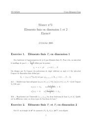
Métho<strong>de</strong> <strong>de</strong>s différences finies.Métho<strong>de</strong> <strong>de</strong>s différences finies: le principe.Points <strong>de</strong> <strong>calcul</strong>: x j = j ∆x, 0 ≤ j ≤ J + 1, t n = n∆t, n ≥ 0.Pour produire <strong>les</strong> équations définissant <strong>les</strong> inconnuesdiscrètes, l’idée est d’écrire (<strong>de</strong> façon approchée) l’<strong>EDP</strong> àrésoudre en chaque point intérieur <strong>de</strong> <strong>la</strong> grille <strong>de</strong> <strong>calcul</strong>.¡u n jt n∆tPour ce<strong>la</strong> il f<strong>au</strong>t définir <strong>de</strong>s approximations d’opérateursdifférentiels ne faisant appel qu’<strong>au</strong>x valeurs discrètes:ce sont <strong>les</strong> opérateurs <strong>au</strong>x différences.Les équations manquantes sont fournies par <strong>la</strong> prise encompte <strong>de</strong>s conditions initia<strong>les</strong> et <strong>de</strong>s conditions <strong>au</strong>x limites.Après discrétisation, on est ramené à <strong>la</strong> résolution d’unproblème posé en dimension finie, traitable sur ordinateur.0 L∆xx j<strong>Introduction</strong> <strong>au</strong> <strong>calcul</strong> <strong>scientifique</strong> <strong>pour</strong> <strong>les</strong> <strong>EDP</strong> <strong>de</strong> <strong>la</strong> physique. – p.15/27<strong>Introduction</strong> <strong>au</strong> <strong>calcul</strong> <strong>scientifique</strong> <strong>pour</strong> <strong>les</strong> <strong>EDP</strong> <strong>de</strong> <strong>la</strong> physique. – p.16/27Construction d’opérateurs <strong>au</strong>x différences.Construction d’opérateurs <strong>au</strong>x différences.L’idée <strong>de</strong> base est <strong>de</strong> revenir à <strong>la</strong> définition d’une dérivéef ′ f(x + h) − f(x) f(x + h) − f(x − h)(x) = lim, = lim, ...h→0 hh→0 2hApproximation <strong>de</strong> ∂u∂t (x j, t n ).∂u∂t (x j, t n ) ∼ un+1 j − u n j∆tC’est une approximation décentrée à droite,l’erreur <strong>de</strong> troncatured’ordre 1 carε n j = u(x j, t n+1 ) − u(x j , t n )− ∂u∆t∂t (x j, t n )(Taylor) = ∆t ∂ 2 u2 ∂t (x j, t n ) + O(∆t 2 )2<strong>Introduction</strong> <strong>au</strong> <strong>calcul</strong> <strong>scientifique</strong> <strong>pour</strong> <strong>les</strong> <strong>EDP</strong> <strong>de</strong> <strong>la</strong> physique. – p.17/27<strong>Introduction</strong> <strong>au</strong> <strong>calcul</strong> <strong>scientifique</strong> <strong>pour</strong> <strong>les</strong> <strong>EDP</strong> <strong>de</strong> <strong>la</strong> physique. – p.17/27
Construction d’opérateurs <strong>au</strong>x différences.Approximation <strong>de</strong> ∂ ( ∂u) σ (xj , t n ).∂x ∂xConstruction d’opérateurs <strong>au</strong>x différences.Supposons connu v n j+ 1 2= v(x j+1 , t n ), v = σ ∂u2∂x .On réalise alors une approximation centrée, d’ordre 2 avec:∂ ( ∂u) σ (xj , t n ) = ∂v v n − v n∂x ∂x ∂x (x j, t n j+) ∼1 j− 1 22∆xOn fait alors l’approximation (centrée):v n j+ 1 2u n j+1 − u n j∼ σ j+12 ∆x<strong>pour</strong> aboutir à:∂∂x( ∂u) σ (xj , t n ) ∼ 1 (∂x ∆xσ j+12( un j+1 − u n j∆x) − σ j−1 ( un j − u n )j−1)2 ∆x<strong>Introduction</strong> <strong>au</strong> <strong>calcul</strong> <strong>scientifique</strong> <strong>pour</strong> <strong>les</strong> <strong>EDP</strong> <strong>de</strong> <strong>la</strong> physique. – p.18/27<strong>Introduction</strong> <strong>au</strong> <strong>calcul</strong> <strong>scientifique</strong> <strong>pour</strong> <strong>les</strong> <strong>EDP</strong> <strong>de</strong> <strong>la</strong> physique. – p.18/27Construction d’opérateurs <strong>au</strong>x différences.Le schéma numériqueLorsque σ est constant on a fait l’approximation:Pour n ≥ 0 et 1 ≤ j ≤ J − 1:σ ∂2 u∂x (x j, t n ) ∼ σ un j+1 − 2u n j + u n j−12 ∆x 2qui est une approximation d’ordre 2 ainsi que le montrel’estimation <strong>de</strong> l’erreur <strong>de</strong> troncature:ε n j = σ u(x j+1, t n ) − 2u(x j , t n ) + u(x j−1 , t n )∆x 2∣ = σ ∆x2 ∂ 4 u12 ∂x (x j, t n ) + O(∆x 4 )4− σ ∂2 u∂x 2 (x j, t n )u n+1j− u n j∆t⎧⎪⎨⎪⎩− 1 (∆xσ j+12( un j+1 − u n j∆xPour 1 ≤ j ≤ J − 1: u 0 j = u 0,j .Pour n ≥ 0: u n 0 = u n l .Pour n ≥ 0:) − σ j−1 ( un j − u n )j−1) = 0.2 ∆xu n J − un J−1∆x= q n l .<strong>Introduction</strong> <strong>au</strong> <strong>calcul</strong> <strong>scientifique</strong> <strong>pour</strong> <strong>les</strong> <strong>EDP</strong> <strong>de</strong> <strong>la</strong> physique. – p.19/27<strong>Introduction</strong> <strong>au</strong> <strong>calcul</strong> <strong>scientifique</strong> <strong>pour</strong> <strong>les</strong> <strong>EDP</strong> <strong>de</strong> <strong>la</strong> physique. – p.20/27
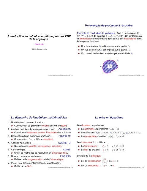
¢¢¢¢¢¥¥¥¥¥Le schéma numériqueMise en oeuvre du schéma numérique.Pour n ≥ 0 et 1 ≤ j ≤ J − 1:On construit <strong>la</strong> grille <strong>de</strong> <strong>calcul</strong>.u n+1j= u n j + ∆t∆x 2 (σ j+12)(u n j+1 − u n j ) − σ j−1 (u n j − u n j−1) = 0.2⎧⎪⎨⎪⎩Pour 1 ≤ j ≤ J − 1: u 0 j = u 0,j .Pour n ≥ 0: u n 0 = u n l .Pour n ≥ 0: u n J = un J−1 + ∆x qn l .∆tIl s’agit d’un schéma explicite.∆x<strong>Introduction</strong> <strong>au</strong> <strong>calcul</strong> <strong>scientifique</strong> <strong>pour</strong> <strong>les</strong> <strong>EDP</strong> <strong>de</strong> <strong>la</strong> physique. – p.20/27<strong>Introduction</strong> <strong>au</strong> <strong>calcul</strong> <strong>scientifique</strong> <strong>pour</strong> <strong>les</strong> <strong>EDP</strong> <strong>de</strong> <strong>la</strong> physique. – p.21/27Mise en oeuvre du schéma numérique.Mise en oeuvre du schéma numérique.On prend en compte <strong>les</strong> condition initiale et <strong>de</strong> Dirichlet.Supposons <strong>la</strong> solution <strong>calcul</strong>ée jusqu’à l’instant t n .§ § § § § § § § § §£ £ £ £ £ £ £ £ £ ££ £ £ £ £ £ £ £ £ £§ § § § § § § § § §£ £ £ £ £ £ £ £ £ ££ £ £ £ £ £ £ £ £ £∆t§ § § § § § § § § §¦ ¦ ¦ ¦ ¦ ¦ ¦ ¦ ¦ ¦t n+1t n¦ ¦ ¦ ¦ ¦ ¦ ¦ ¦ ¦ ¦£ £ £ £ £ £ £ £ £ £¥¤ ¤ ¤ ¤ ¤ ¤ ¤ ¤ ¤ ¤ ¤¢¡¡¡¡¡¡¡¡¡¡¡∆x<strong>Introduction</strong> <strong>au</strong> <strong>calcul</strong> <strong>scientifique</strong> <strong>pour</strong> <strong>les</strong> <strong>EDP</strong> <strong>de</strong> <strong>la</strong> physique. – p.21/27<strong>Introduction</strong> <strong>au</strong> <strong>calcul</strong> <strong>scientifique</strong> <strong>pour</strong> <strong>les</strong> <strong>EDP</strong> <strong>de</strong> <strong>la</strong> physique. – p.21/27
L’analyse numérique.C’est une branche <strong>de</strong>s mathématiques qui s’est développéeavec l’avènement <strong>de</strong>s ordinateurs.L’analyse numérique <strong>de</strong>s équations <strong>au</strong>x dérivées partiel<strong>les</strong> estl’art <strong>de</strong> maîtriser le passage du continu <strong>au</strong> discret.Montrer que le problème approché est bien posé:existence et unicité <strong>de</strong> u h .Montrer <strong>la</strong> convergence : u h → u quand h → 0.La stabilité : borne uniforme du type ‖u h ‖ ≤ C.La consistance : approximation <strong>de</strong>s équations.Un exemple <strong>de</strong> schéma instable.Revenons à notre problème modèle. Pour améliorer <strong>la</strong>précision <strong>de</strong> notre métho<strong>de</strong> on peut penser à utiliser uneapproximation centrée <strong>de</strong> <strong>la</strong> dérivée en temps.u n+1j− u n−1j2∆t− 1 (∆xσ j+12( un j+1 − u n j∆x) − σ j−1 ( un j − u n )j−1) = 0.2 ∆xUn tel schéma se révèle inconditionnellement instable.Obtenir <strong>de</strong>s estimations d’erreur: ‖u − u h ‖ ≤ ? .En principe : stabilité + consistance =⇒ convergence.<strong>Introduction</strong> <strong>au</strong> <strong>calcul</strong> <strong>scientifique</strong> <strong>pour</strong> <strong>les</strong> <strong>EDP</strong> <strong>de</strong> <strong>la</strong> physique. – p.22/27<strong>Introduction</strong> <strong>au</strong> <strong>calcul</strong> <strong>scientifique</strong> <strong>pour</strong> <strong>les</strong> <strong>EDP</strong> <strong>de</strong> <strong>la</strong> physique. – p.23/27Autres exemp<strong>les</strong>.Problèmes stationnaires elliptiques.Nous faisons l’hypothèse que quand t → +∞:⎧⎨ θ l (x, t) → θ ∞ l (x) x ∈ Γ 0⎩q l (x, t) → q ∞ l (x) x ∈ Γ 1On peut démontrer <strong>la</strong> convergence vers un état stationnaireθ(x, t) → θ ∞ (x),t → +∞,où θ ∞ : Ω → R est solution du problème <strong>au</strong>x limites:Autres exemp<strong>les</strong>.Problèmes stationnaires elliptiques.On peut démontrer <strong>la</strong> convergence vers un état stationnaireθ(x, t) → θ ∞ (x),t → +∞,où θ ∞ : Ω → R est solution du problème <strong>au</strong>x limites:⎧−div ( σ∇θ ∞) = 0, dans Ω,⎪⎨θ ∞ = θ l , sur Γ 0 ,⎪⎩ σ ∂θ∞∂n = q l, sur Γ 0 .<strong>Introduction</strong> <strong>au</strong> <strong>calcul</strong> <strong>scientifique</strong> <strong>pour</strong> <strong>les</strong> <strong>EDP</strong> <strong>de</strong> <strong>la</strong> physique. – p.24/27<strong>Introduction</strong> <strong>au</strong> <strong>calcul</strong> <strong>scientifique</strong> <strong>pour</strong> <strong>les</strong> <strong>EDP</strong> <strong>de</strong> <strong>la</strong> physique. – p.24/27
Autres exemp<strong>les</strong>.Problèmes stationnaires elliptiques.Autres exemp<strong>les</strong>.Problèmes hyperboliques linéaires. (Cours 9 et 10)⎧⎪⎨⎪⎩−div ( σ∇θ ∞) = 0, dans Ω,θ ∞ = θ l , sur Γ 0 ,σ ∂θ∞∂n = q l, sur Γ 0 .La propagation du son dans un flui<strong>de</strong> est régie par l’équation<strong>de</strong>s on<strong>de</strong>s acoustiques:1ρ 0 c 2 0∂ 2 p∂t 2 − div( 1ρ 0∇p ) = f,où l’inconnue p désigne <strong>la</strong> (variation <strong>de</strong>) pression, ρ 0 désigne <strong>la</strong><strong>de</strong>nsité du flui<strong>de</strong>, c 0 <strong>la</strong> célérité du son et f un terme source.Ce problème est le prototype <strong>de</strong>s problèmes elliptiques qu’onrecontre <strong>au</strong>ssi en mécanique <strong>de</strong>s soli<strong>de</strong>s et <strong>de</strong>s flui<strong>de</strong>s(phénomènes d’equilibre), en électrostatique,...Seront étudiés dans <strong>les</strong> cours 2,3,4,5.Au même titre que l´équation <strong>de</strong> transport, l’équation <strong>de</strong>son<strong>de</strong>s est le prototype <strong>de</strong> l’équation hyperbolique linéairequi décrit <strong>de</strong>s phénomènes <strong>de</strong> propagation.On rencontre <strong>au</strong>ssi ce type d’équation en électromagnétisme(Maxwell) ou en mécanique du soli<strong>de</strong> (é<strong>la</strong>stodynamique).<strong>Introduction</strong> <strong>au</strong> <strong>calcul</strong> <strong>scientifique</strong> <strong>pour</strong> <strong>les</strong> <strong>EDP</strong> <strong>de</strong> <strong>la</strong> physique. – p.24/27<strong>Introduction</strong> <strong>au</strong> <strong>calcul</strong> <strong>scientifique</strong> <strong>pour</strong> <strong>les</strong> <strong>EDP</strong> <strong>de</strong> <strong>la</strong> physique. – p.25/27Problèmes <strong>de</strong> type Fredholm.Autres exemp<strong>les</strong>.Si le terme source est harmonique en temps:f(x, t) = f ∞ (x) exp iωtoù <strong>la</strong> pulsation ω > 0 est donnée, on <strong>au</strong>ra le comportement entemps long:p(x, t) ∼ p ∞ (x) exp iωt,t → +∞.où p ∞ est solution <strong>de</strong> l’équation <strong>de</strong> Helmholtz:−div ( 1 ) ω 2∇p ∞ − pρ 0 ρ 0 c 2 ∞ = f ∞ (x).0C’est le prototype du problème elliptique non coercif mais <strong>de</strong>type Fredholm, traité dans <strong>les</strong> cours 6 et 7.<strong>Introduction</strong> <strong>au</strong> <strong>calcul</strong> <strong>scientifique</strong> <strong>pour</strong> <strong>les</strong> <strong>EDP</strong> <strong>de</strong> <strong>la</strong> physique. – p.26/27Autres exemp<strong>les</strong>.Problèmes hyperboliques non linéaires.Ces modè<strong>les</strong> interviennent <strong>pour</strong> <strong>la</strong> <strong>de</strong>scription <strong>de</strong>sphénomènes <strong>de</strong> propagation non linéaire, surtout enmécanique <strong>de</strong>s flui<strong>de</strong>s (propagation <strong>de</strong>s chocs, on<strong>de</strong>s<strong>de</strong> détente,...) mais <strong>au</strong>ssi <strong>pour</strong> <strong>la</strong> modélisation du trafficroutier (modélisation <strong>de</strong>s bouchons).En dimension 1, l’équation modèle est (f : R → R):f(u) = <strong>au</strong>f(u) = u 2 /2∂u∂t + ∂ f(u) = 0, x ∈ R, t > 0.∂x: équation <strong>de</strong> transport.: équation <strong>de</strong> Burgers.Cette équation sera traitée <strong>au</strong>x cours 11 et 12.<strong>Introduction</strong> <strong>au</strong> <strong>calcul</strong> <strong>scientifique</strong> <strong>pour</strong> <strong>les</strong> <strong>EDP</strong> <strong>de</strong> <strong>la</strong> physique. – p.27/27