1.1 Generalit`a dei controllori PID - Dipartimento di Ingegneria dell ...
1.1 Generalit`a dei controllori PID - Dipartimento di Ingegneria dell ...
1.1 Generalit`a dei controllori PID - Dipartimento di Ingegneria dell ...

Create successful ePaper yourself
Turn your PDF publications into a flip-book with our unique Google optimized e-Paper software.
I Controllori <strong>PID</strong> (ver. 1.0)<br />
<strong>1.1</strong> Generalità <strong>dei</strong> <strong>controllori</strong> <strong>PID</strong><br />
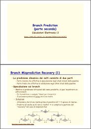
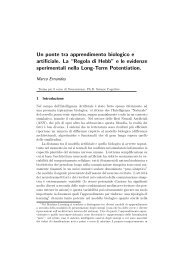
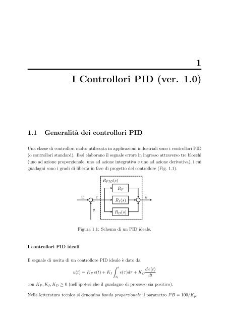
Una classe <strong>di</strong> <strong>controllori</strong> molto utilizzata in applicazioni industriali sono i <strong>controllori</strong> <strong>PID</strong><br />
(o <strong>controllori</strong> standard). Essi elaborano il segnale errore in ingresso attraverso tre blocchi<br />
(uno ad azione proporzionale, uno ad azione integrativa e uno ad azione derivativa), i cui<br />
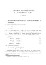
guadagni sono i gra<strong>di</strong> <strong>di</strong> libertà in fase <strong>di</strong> progetto del controllore (Fig. <strong>1.1</strong>).<br />
I <strong>controllori</strong> <strong>PID</strong> ideali<br />
w<br />
−<br />
y<br />
e<br />
R<strong>PID</strong>(s)<br />
RP<br />
RI(s)<br />
RD(s)<br />
Figura <strong>1.1</strong>: Schema <strong>di</strong> un <strong>PID</strong> ideale.<br />
Il segnale <strong>di</strong> uscita <strong>di</strong> un controllore <strong>PID</strong> ideale è dato da:<br />
u(t) = KP e(t) + KI<br />
t<br />
t0<br />
u<br />
de(t)<br />
e(τ)dτ + KD<br />
dt<br />
con KP,KI,KD ≥ 0 (nell’ipotesi che il guadagno <strong>di</strong> processo sia positivo).<br />
Nella letteratura tecnica si denomina banda proporzionale il parametro PB = 100/Kp.<br />
1
2 I Controllori <strong>PID</strong> (ver. 1.0)<br />
La funzione <strong>di</strong> trasferimento <strong>di</strong> un <strong>PID</strong> ideale è:<br />
R<strong>PID</strong>(s) = KP + KI<br />
s + KDs = KDs2 + KPs + KI<br />
. (<strong>1.1</strong>)<br />
s<br />
Una forma alternativa alla (<strong>1.1</strong>) più utilizzata in pratica è la seguente:<br />
R<strong>PID</strong>(s) = KP<br />
<br />
1 + 1<br />
<br />
+ TDs = KP<br />
TIs<br />
TI = KP/KI ←→ costante <strong>di</strong> tempo integrale (o <strong>di</strong> reset).<br />
TD = KD/KP ←→ costante <strong>di</strong> tempo derivativa.<br />
Realizzazione causale <strong>dei</strong> <strong>controllori</strong> <strong>PID</strong><br />
<br />
TITDs2 <br />
+ TIs + 1<br />
TIs<br />
(1.2)<br />
Poiché le funzioni <strong>di</strong> trasferimento (<strong>1.1</strong>)-(1.2) non sono proprie, risultano irrealizzabili in<br />
pratica.<br />
Per ottenere una funzione <strong>di</strong> trasferimento propria si aggiunge un polo ad alta frequenza<br />
al blocco derivatore ottenendo:<br />
R r <strong>PID</strong>(s) = KP<br />
<br />
1 + 1<br />
TIs<br />
TDs<br />
+<br />
1 + TD<br />
N s<br />
<br />
= KP + KI<br />
s<br />
+ KDs<br />
1 + KD<br />
KP N s.<br />
La costante positiva N è scelta in modo tale che il polo s = −N/TD sia fuori dalla banda<br />
del controllo (N = 5 ÷ 20).<br />
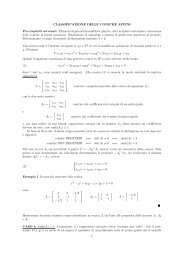
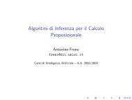
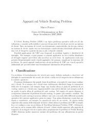
In Fig. <strong>1.1</strong> sono riportate le risposte in frequenza <strong>dell</strong>e funzioni <strong>di</strong> trasferimento <strong>di</strong> un<br />
<strong>PID</strong> ideale e reale.<br />
In genere, nel seguito faremo riferimento sempre alla forma ideale.<br />
Casi particolari<br />
Casi particolari sono i regolatori P, PI e PD.<br />
RP = KP<br />
RPI(s) = KPs + KI<br />
s<br />
= KP<br />
1 + TIs<br />
TIs
1.2 Aspetti realizzativi <strong>dei</strong> <strong>controllori</strong> <strong>PID</strong> 3<br />
Modulo<br />
Fase<br />
70<br />
60<br />
50<br />
40<br />
30<br />
20<br />
10<br />
100<br />
50<br />
0<br />
−50<br />
10 −2<br />
−100<br />
10 −1<br />
10 0<br />
Figura 1.2: Diagramma <strong>di</strong> Bode <strong>di</strong> un controllore <strong>PID</strong> ideale (−) e reale (− −).<br />
10 1<br />
10 2<br />
R i P ID<br />
R r P ID<br />
R i P ID<br />
R r P ID<br />
RPD(s) = KP + KDs = KP(1 + TDs)<br />
I regolatori <strong>PID</strong> ideali hanno un polo nell’origine e 2 zeri in<br />
z1,2 = −TI ± TI(TI − 4TD)<br />
2TITD<br />
Al variare <strong>dei</strong> parametri, i due zeri possono essere complessi, reali <strong>di</strong>stinti o reali coinci-<br />
denti (se Ti = 4TD). Spesso, per semplificare la taratura, si preferisce avere 2 zeri reali<br />
coincidenti.<br />
1.2 Aspetti realizzativi <strong>dei</strong> <strong>controllori</strong> <strong>PID</strong><br />
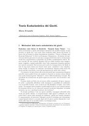
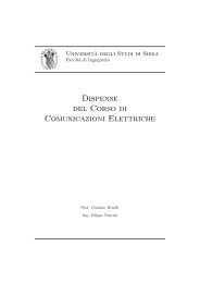
Poiché il riferimento in un sistema controllato può contenere segnali a gra<strong>di</strong>no o comunque<br />
segnali con rapida variazione, negli istanti in cui si ha una variazione, il blocco derivatore<br />
fornisce un contributo al segnale <strong>di</strong> attuazione molto elevato. Si usa allora sottoporre ad<br />
azione derivativa l’uscita y piuttosto che il segnale <strong>di</strong> errore e (Fig. 1.2b).<br />
Vale che:<br />
• I poli ad anello chiuso <strong>dell</strong>e due configurazioni sono gli stessi.<br />
10 3
4 I Controllori <strong>PID</strong> (ver. 1.0)<br />
R<strong>PID</strong>(s)<br />
RP<br />
d<br />
RP<br />
d<br />
w e<br />
−<br />
RI<br />
u<br />
G(s)<br />
y w e<br />
−<br />
RI<br />
u<br />
−<br />
G(s)<br />
y<br />
RD<br />
R<strong>PID</strong>(s)<br />
RD<br />
a b<br />
Figura 1.3: Controllore <strong>PID</strong> con azione derivativa sul segnale <strong>di</strong> errore (a), e sull’uscita<br />
(b).<br />
• Le funzioni <strong>di</strong> trasferimento S(s) = Y (s)/D(s) e Q(s) = U(s)/D(s) sono identiche<br />
nelle due configurazioni.<br />
Infatti, nel caso <strong>di</strong> Fig. 1.2a si ha:<br />
Y (s) = R<strong>PID</strong>(s)G(s)<br />
1<br />
W(s) +<br />
1 + R<strong>PID</strong>(s)G(s) 1 + R<strong>PID</strong>(s)G(s) D(s)<br />
U(s) =<br />
R<strong>PID</strong>(s)<br />
[W(s) − D(s)] ,<br />
1 + R<strong>PID</strong>(s)G(s)<br />
mentre per quanto riguarda il caso in Fig. 1.2b, risulta:<br />
Y (s) =<br />
U(s) =<br />
RPI(s)G(s)<br />
1<br />
W(s) +<br />
1 + R<strong>PID</strong>(s)G(s) 1 + R<strong>PID</strong>(s)G(s) D(s)<br />
RPI(s)<br />
R<strong>PID</strong>(s)<br />
W(s) −<br />
1 + R<strong>PID</strong>(s)G(s) 1 + R<strong>PID</strong>(s)G(s) D(s).<br />
• F(s) = Y (s)/W(s) ha sempre guadagno unitario e S(s) ha uno zero nell’origine;<br />
quin<strong>di</strong> il sistema riesce ancora ad inseguire un riferimento a gra<strong>di</strong>no senza errori e<br />
garantire la reiezione <strong>dei</strong> <strong>di</strong>sturbi costanti.<br />
Esempio <strong>1.1</strong><br />
G(s) =<br />
5<br />
(s + 1) 2 (s + 3) .<br />
Consideriamo un R<strong>PID</strong> con: KP = 3, KI = 2, KD = 1 (TI = 3/2, TD = 1/3), ovvero<br />
R<strong>PID</strong>(s) =<br />
L(s) = R<strong>PID</strong>(s)G(s) =<br />
(s + 1)(s + 2)<br />
s<br />
5 (s + 2)<br />
s(s + 1)(s + 3) ,
1.2 Aspetti realizzativi <strong>dei</strong> <strong>controllori</strong> <strong>PID</strong> 5<br />
per cui si ha:<br />
ωc 1.84rad/s , φm 40 ◦ , Km → ∞,<br />
dove con ωc denotiamo la frequenza <strong>di</strong> attraversamento degli 0dB, con φm il margine <strong>di</strong><br />
fase e con Km il margine <strong>di</strong> guadagno.<br />
Se si considera un <strong>PID</strong> reale con N = 5 (polo aggiuntivo in −N/TD = −15) si ottiene:<br />
ωc 1.92rad/s , φm 37 ◦ , Km 17dB.<br />
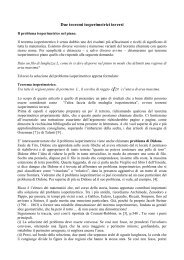
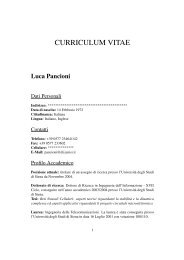
E’ interessante notare l’andamento <strong>di</strong> y ed u per le due realizzazioni (derivazione <strong>di</strong> e o<br />
<strong>di</strong> y) del controllore in corrispondenza ad un ingresso a gra<strong>di</strong>no.<br />
1.5<br />
1<br />
0.5<br />
0<br />
0 1 2 3 4 5 6 7 8 9 10<br />
Tempo (s)<br />
18<br />
16<br />
14<br />
12<br />
10<br />
8<br />
6<br />
4<br />
2<br />
0<br />
−2<br />
0 1 2 3 4 5 6 7 8 9 10<br />
Tempo (s)<br />
a b<br />
Figura 1.4: (a) Risposta al gra<strong>di</strong>no del sistema <strong>dell</strong>’esempio <strong>1.1</strong> con azione derivativa<br />
sull’errore (−) e sull’uscita (− −). (b) Relativo segnale <strong>di</strong> comando u(t) per i due casi.<br />
Scelta del valore <strong>di</strong> N<br />
Come enunciato in precedenza, la scelta <strong>di</strong> N determina la posizione del polo aggiuntivo.<br />
Poiché al crescere <strong>di</strong> N, R r <strong>PID</strong> → R<strong>PID</strong>, e |R<strong>PID</strong>(jω)| → ∞ per ω → ∞, allora per<br />
moderare l’eccitazione del comando da parte <strong>di</strong> componenti ad alta frequenza <strong>dei</strong> <strong>di</strong>sturbi<br />
in anello d, bisogna selezionare N il più basso possibile, compatibilmente con il posizionare<br />
il polo aggiuntivo fuori dalla banda del controllo.<br />
A titolo esemplificativo, vale la pena osservare gli andamenti <strong>di</strong> y e u per N = 5 e N = 30<br />
nel caso in cui il sistema <strong>di</strong> controllo <strong>dell</strong>’esempio <strong>1.1</strong> venga sottoposto ad un <strong>di</strong>sturbo
6 I Controllori <strong>PID</strong> (ver. 1.0)<br />
d a spettro costante. In Fig. 1.5 viene riportata l’uscita del sistema per le due scelte <strong>di</strong><br />
N; notare che le due uscite sono quasi perfettamente coincidenti. In Fig. 1.6 sono invece<br />
riportati i valori del comando; in questo caso si può notare come la scelta <strong>di</strong> un valore <strong>di</strong><br />
N = 5 risulti decisamente migliore.<br />
1.6<br />
1.4<br />
1.2<br />
1<br />
0.8<br />
0.6<br />
0.4<br />
0.2<br />
0<br />
−0.2<br />
0 1 2 3 4 5<br />
Tempo (s)<br />
6 7 8 9 10<br />
Figura 1.5: Andamento <strong>di</strong> w e y nell’esempio <strong>1.1</strong> con lo schema <strong>di</strong> derivazione <strong>dell</strong>’uscita<br />
per N = 5 (−) e N = 30 (− −).<br />
u<br />
10<br />
8<br />
6<br />
4<br />
2<br />
0<br />
−2<br />
−4<br />
−6<br />
−8<br />
−10<br />
0 1 2 3 4 5<br />
Tempo (s)<br />
6 7 8 9 10<br />
u<br />
10<br />
8<br />
6<br />
4<br />
2<br />
0<br />
−2<br />
−4<br />
−6<br />
−8<br />
−10<br />
0 1 2 3 4 5<br />
Tempo (s)<br />
6 7 8 9 10<br />
a b<br />
Figura 1.6: (a) Andamento del comando u per N = 5. (b) Andamento del comando u<br />
per N = 30.<br />
1.2.1 Struttura <strong>dei</strong> <strong>PID</strong> industriali<br />
Per evitare <strong>di</strong> sollecitare molto la variabile <strong>di</strong> comando, a volte anche l’azione proporzio-<br />
nale è applicata solo a y, invece che a e. In generale, in ambito industriale, i regolatori
1.3 Desaturazione <strong>dell</strong>’azione integrale (schemi anti-windup) 7<br />
<strong>PID</strong> sono strutturati in maniera flessibile, in modo da rendere agevole la loro taratura.<br />
In particolare:<br />
dove: ⎧ ⎪⎨<br />
U(s) = KPEP(s) + KI<br />
s E(s) + KDsED(s) ,<br />
⎪⎩<br />
E(s) = W(s) − Y (s)<br />
EP(s) = αW(s) − Y (s)<br />
ED(s) = βW(s) − Y (s)<br />
I parametri α e β sono scelti in modo da ottimizzare le prestazioni del sistema <strong>di</strong> controllo.<br />
Poiché l’analisi fatta in precedenza per lo schema del <strong>PID</strong> con azione derivativa sull’uscita<br />
può essere estesa a qualunque α e β, se ne deduce che al variare <strong>di</strong> α e β, mentre la<br />
posizione <strong>dei</strong> poli del sistema ad anello chiuso non varia, cambiano invece gli zeri <strong>di</strong><br />
Y (s)/W(s) e U(s)/W(s), e <strong>di</strong> conseguenza le prestazioni del sistema.<br />
1.3 Desaturazione <strong>dell</strong>’azione integrale (schemi anti-<br />
windup)<br />
Gli attuatori utilizzati nei sistemi <strong>di</strong> controllo hanno <strong>dei</strong> vincoli sull’ampiezza <strong>dell</strong>e uscite,<br />
che non possono superare <strong>dei</strong> valori massimi e minimi. Quando si utilizza un regolatore<br />
con azione integrale, è possibile che l’uscita del controllore raggiunga i suddetti vincoli; in<br />
tal caso l’azione <strong>dell</strong>’attuatore non può crescere, anche se l’errore <strong>di</strong> regolazione e(t) non<br />
è nullo.<br />
Assumiamo per como<strong>di</strong>tà <strong>di</strong> avere un compensatore puramente integrale del tipo KI/s.<br />
La situazione reale che spesso si incontra è quella riportata in Fig. 1.7 (attuatore in<br />
saturazione), in cui:<br />
Il fenomeno del wind-up<br />
⎧<br />
⎪⎨ −UM , se u(t) < −UM<br />
m(t) = u(t)<br />
⎪⎩<br />
UM<br />
, se |u(t)| ≤ UM<br />
, se u(t) > UM<br />
In presenza <strong>di</strong> saturazione, come detto in precedenza, può verificarsi che l’uscita <strong>dell</strong>’attua-<br />
tore non cresca, pur rimanendo l’errore <strong>di</strong> regolazione e(t) non nullo. Conseguentemente,<br />
il termine integrale continua a crescere, ma tale incremento non produce alcun effetto
8 I Controllori <strong>PID</strong> (ver. 1.0)<br />
w(t)<br />
−<br />
uM e(t)<br />
KI s<br />
u(t)<br />
m(t)<br />
−u M<br />
G(s)<br />
Figura 1.7: Schema in cui l’attuatore presenta una saturazione.<br />
sulla variabile <strong>di</strong> comando <strong>dell</strong>’impianto. Tale situazione, oltre a non far funzionare cor-<br />
rettamente il regolatore, rende inattivo il regolatore anche quando l’errore <strong>di</strong>minuisce o si<br />
inverte <strong>di</strong> segno; infatti, il sistema <strong>di</strong> regolazione può riattivarsi solo allorquando il segnale<br />
u(t) rientra nella zona <strong>di</strong> linearità <strong>dell</strong>a caratteristica <strong>dell</strong>’attuatore (scarica del termine<br />
integrale). Questo fenomeno si chiama comunemente carica integrale o integral wind-up.<br />
Esempio 1.2<br />
Sia data la seguente funzione <strong>di</strong> trasferimento:<br />
G(s) = 4<br />
s + 2 .<br />
Assumiamo <strong>di</strong> utilizzare un controllore integrale con KI = 1. In con<strong>di</strong>zioni <strong>di</strong> linearità<br />
risulta:<br />
ωc 1.57rad/s , φm 52 ◦ .<br />
Supponiamo adesso che l’attuatore presenti una saturazione con UM = 0.53. I risultati<br />
<strong>dell</strong>a simulazione per un ingresso a gra<strong>di</strong>no sono mostrati in Fig. 1.8.<br />
Schema <strong>di</strong> desaturazione<br />
Il problema del wind-up può essere evitato interrompendo l’azione integrale non appena<br />
l’uscita del controllore raggiunge il livello <strong>di</strong> saturazione <strong>dell</strong>’attuatore.<br />
Una possibile soluzione è riportata in Fig. 1.9.<br />
Supponiamo che il controllore <strong>PID</strong> che deve essere realizzato sia <strong>dell</strong>a forma generale<br />
R<strong>PID</strong>(s) = NR(s)<br />
DR(s) , con DR(0) = 0,<br />
in cui la con<strong>di</strong>zione DR(0) = 0 implica la presenza <strong>di</strong> un blocco integrale nel controllore.<br />
Supponiamo che sia NR(0) > 0. Allora, riferendosi allo schema riportato in Fig. 1.9, si<br />
y(t)
1.3 Desaturazione <strong>dell</strong>’azione integrale (schemi anti-windup) 9<br />
1.4<br />
1.2<br />
1<br />
0.8<br />
0.6<br />
0.4<br />
0.2<br />
0<br />
0 1 2 3 4 5 6 7 8 9 10<br />
Tempo (s)<br />
1.2<br />
1<br />
0.8<br />
0.6<br />
0.4<br />
0.2<br />
0<br />
−0.2<br />
0 1 2 3 4 5 6 7 8 9 10<br />
Tempo (s)<br />
a b<br />
Figura 1.8: (a) Risposta <strong>di</strong> un sistema in assenza (−) e in presenza (− −) <strong>di</strong> saturazione.<br />
(b) Andamento <strong>dei</strong> segnali <strong>di</strong> e(t) (−), u(t) (− −) ed m(t) (−.) in presenza <strong>di</strong> saturazione.<br />
w(t)<br />
e(t)<br />
NR(s)<br />
Γ(s)<br />
q(t) u(t)<br />
−<br />
z(t)<br />
Ψ(s)<br />
Figura 1.9: Schema <strong>di</strong> realizzazione <strong>di</strong> un controllore <strong>PID</strong> con <strong>di</strong>spositivo anti wind-up.<br />
sceglie Γ(s) in modo tale che la funzione <strong>di</strong> trasferimento<br />
Ψ(s) =<br />
u M<br />
Γ(s) − DR(s)<br />
Γ(s)<br />
sia asintoticamente stabile, strettamente propria e con guadagno unitario (Ψ(0) = 1). Si<br />
può allora osservare che:<br />
−u M<br />
m(t)<br />
G(s)<br />
• Se l’attuatore opera in regione <strong>di</strong> linearità, la funzione <strong>di</strong> trasferimento fra e(t) e<br />
m(t) coincide con la R<strong>PID</strong>(s) desiderata.<br />
• Se il segnale errore e(t) permane <strong>dell</strong>o stesso segno per un tempo elevato, allora<br />
anche q(t), in funzione <strong>dell</strong>a <strong>di</strong>namica <strong>di</strong> Γ(s), assumerà lo stesso segno; m(t) satura<br />
y(t)
10 I Controllori <strong>PID</strong> (ver. 1.0)<br />
al valore massimo UM <strong>dell</strong>’attuatore. Dato che Ψ(0) = 1, anche z(t) si assesterà al<br />
valore UM, sempre con una <strong>di</strong>namica che <strong>di</strong>pende da Γ(s). Se e(t) cambia <strong>di</strong> segno,<br />
anche q(t) cambia segno e quin<strong>di</strong> il segnale u(t) = q(t) + z(t) scende subito sotto<br />
il valore <strong>di</strong> saturazione UM, attivando il comportamento lineare <strong>dell</strong>’attuatore. Le<br />
prestazioni del sistema <strong>di</strong> desaturazione <strong>di</strong>pendono dalla scelta del polinomio Γ(s),<br />
che costituisce il nucleo del progetto del desaturatore.<br />
Esempio 1.3<br />
Facendo riferimento alle funzioni <strong>dell</strong>’esempio 1.2, assumiamo:<br />
Γ(s) = s + 8 =⇒ Ψ(s) = 8<br />
s + 8 .<br />
La risposta del sistema desaturato è riportata in Fig. <strong>1.1</strong>0.<br />
1.4<br />
1.2<br />
1<br />
0.8<br />
0.6<br />
0.4<br />
0.2<br />
0<br />
0 1 2 3 4 5 6 7 8 9 10<br />
Tempo (s)<br />
Figura <strong>1.1</strong>0: Risposta del sistema senza saturazione (-), con saturazione (–) e con<br />
saturazione e anti wind-up (-.).<br />
Specializzando il caso generale al caso PI, si ha che una scelta generale è:<br />
RPI(s) = KP s + KI<br />
s<br />
= KP<br />
1 + TI s<br />
TI s<br />
=⇒ Γ(s) = 1 + s TI
1.3 Desaturazione <strong>dell</strong>’azione integrale (schemi anti-windup) 11<br />
w(t)<br />
e(t) q(t) u(t)<br />
KP<br />
−<br />
z(t)<br />
u M<br />
1<br />
1+sTI<br />
m(t)<br />
KP sTD<br />
1+ s T D<br />
N<br />
G(s)<br />
Figura <strong>1.1</strong>1: Schema generale <strong>di</strong> anti wind-up per un controllore PI.<br />
−u M<br />
1.3.1 Meto<strong>di</strong> <strong>di</strong> taratura automatica<br />
In molte applicazioni industriali, la costruzione <strong>di</strong> un buon mo<strong>dell</strong>o <strong>dell</strong>’impianto può<br />
essere piuttosto onerosa, soprattutto a fronte <strong>di</strong> esigenze <strong>di</strong> controllo non particolarmente<br />
spinte. Per questi casi sono <strong>di</strong>sponibili <strong>dell</strong>e tecniche <strong>di</strong> taratura <strong>dei</strong> parametri del <strong>PID</strong><br />
(KP, TI e TD) che fanno riferimento a poche e semplici prove da eseguirsi sull’impianto.<br />
Il metodo più classico utilizzato è quello <strong>di</strong> Ziegler-Nichols. Analizzeremo adesso questa<br />
tecnica, sotto le ipotesi che il sistema sia asintoticamente stabile ad anello aperto e abbia<br />
guadagno positivo.<br />
Metodo <strong>di</strong> Ziegler-Nichols (in anello chiuso)<br />
Si chiude il sistema in retroazione su un controllore proporzionale. Fornendo al sistema<br />
un ingresso a gra<strong>di</strong>no, si aumenta il guadagno del controllore finché il sistema oscilla<br />
(con<strong>di</strong>zione critica <strong>di</strong> stabilità). Si in<strong>di</strong>cano con ¯ KP e ¯ T il guadagno critico e il periodo<br />
<strong>dell</strong>’oscillazione <strong>dell</strong>’uscita y(t).<br />
I parametri del regolatore P, PI o <strong>PID</strong> vengono determinati utilizzando la Tabella <strong>1.1</strong>.<br />
R<strong>PID</strong>(s) KP TI TD<br />
P 0.5 ¯ KP<br />
PI 0.45 ¯ KP 0.8 ¯ T<br />
<strong>PID</strong> 0.6 ¯ KP 0.5 ¯ T 0.125 ¯ T<br />
Tabella <strong>1.1</strong>: Tabella <strong>di</strong> Ziegler-Nichols.<br />
y(t)
12 I Controllori <strong>PID</strong> (ver. 1.0)<br />
Notare che se si pone TI = 4TD allora gli zeri del regolatore <strong>PID</strong> sono coincidenti in<br />
posizione s = −4/ ¯ T.<br />
1.4 Interpretazione frequenziale <strong>dei</strong> <strong>PID</strong><br />
La taratura <strong>dei</strong> <strong>PID</strong> col metodo <strong>di</strong> Ziegler-Nichols utilizza due quantità: ¯ KP e ¯ T. Os-<br />
serviamo che la prima quantità è esattamente il margine <strong>di</strong> guadagno (assunto finito)<br />
del sistema controllato G(s), mentre ωπ = 2π/ ¯ T è la pulsazione per cui il <strong>di</strong>agramma<br />
polare G(jω) attraversa il semiasse reale negativo. Si può quin<strong>di</strong> vedere come il control-<br />
lore venga tarato conoscendo soltanto un punto <strong>dell</strong>a risposta in frequenza del sistema<br />
G(jωπ) = −1/ ¯ KP. Per sistemi comuni, tale informazione è sufficiente per progettare<br />
<strong>controllori</strong> che garantiscano prestazioni sod<strong>di</strong>sfacenti.<br />
Esempio 1.4<br />
Consideriamo:<br />
Si può verificare che:<br />
G(s) =<br />
5<br />
(s + 1) 2 (s + 3) .<br />
ωπ = 2.65 , Km = 6.4 =⇒ ¯ KP = 6.4 , ¯ T = 2.37<br />
Dalla Tabella <strong>1.1</strong> risulta, per un controllore PI, KP = 2.88 e TI = 1.9, con i seguenti<br />
in<strong>di</strong>ci <strong>di</strong> prestazione<br />
φm 10.5 ◦ , ωc 1.81rad/s , K ′ m 1.42.<br />
Nel caso <strong>di</strong> un controllore <strong>PID</strong>, con N = 10, i parametri forniti dal metodo <strong>di</strong> Ziegler-<br />
Nichols risultano KP = 3.84, TI = <strong>1.1</strong>9, TD = 0.3 e le relative prestazioni:<br />
φm 27.6 ◦ , ωc 2.14rad/s , K ′ m 10.3.<br />
E’ utile notare come il controllore <strong>PID</strong> abbia aumentato sia il margine <strong>di</strong> guadagno che<br />
quello <strong>di</strong> fase (rispetto al PI).<br />
Valutazione <strong>dell</strong>e prestazioni <strong>di</strong> un <strong>PID</strong><br />
Analizziamo adesso le prestazioni ottenute utilizzando i criteri <strong>di</strong> taratura automatica.
1.4 Interpretazione frequenziale <strong>dei</strong> <strong>PID</strong> 13<br />
• Nell’ipotesi <strong>di</strong> utilizzare un controllore puramente proporzionale, si ottiene che<br />
KPG(jωπ) = 0.5 ¯ KPG(jωπ) = −0.5,<br />
ovvero il controllore proporzionale tarato automaticamente garantisce un margine<br />
<strong>di</strong> guadagno Km pari a 2.<br />
• Nel caso generale, fissata una frequenza ω ∗ , il <strong>di</strong>agramma polare <strong>di</strong> R<strong>PID</strong>(s)G(s)<br />
può essere mo<strong>di</strong>ficato variando i parametri del <strong>PID</strong>, secondo l’effetto in<strong>di</strong>cato in<br />
Fig. <strong>1.1</strong>2.<br />
KI<br />
jω∗G(jω ∗ )<br />
KPG(jω ∗ )<br />
*<br />
ω ∗<br />
jω ∗ KDG(jω ∗ )<br />
Figura <strong>1.1</strong>2: Effetto <strong>dei</strong> termini proporzionale, integrale e derivativo <strong>di</strong> un controllore<br />
<strong>PID</strong>.<br />
In generale si può vedere come il termine derivativo tenda a far aumentare il margine<br />
<strong>di</strong> fase, mentre l’effetto integrativo tende a ridurlo.