analisi bivariata.pdf - Dipartimento di Economia e Statistica

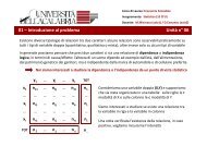
5 – Analisi statistica bivariataDati sul disastro del Titanic (tabella di contingenza)SopravvissutiClasse No Si TotaleI 122 203 325II 167 118 285III 528 178 706Personale 673 212 885Totale 1490 711 2201nij frequenze nella cella di riga i e colonna jni.totale frequenze riga i ( m arg inali riga)n.j totale frequenze colonna j ( m arg inali colonna)N totale frequenze di tabella (2201)

6 – Analisi statistica bivariataSimbologia delle tabelle doppieYy 1 y 2 y 3 ... y j ... y sx 1 n 11 n 12 n 13 ... n 1j ... n 1s n 1.Xx 2 n 21 n 22 n 23 ... n 2j ... n 2s n 2.... ... ... ... ... ... ... ... ...x i n i1 n i2 n i3 ... n ij ... n is n i.... ... ... ... ... ... ... ... ...x r n r1 n r2 n r3 ... n rj ... n rs n r.n .1 n .2 n .3 ... n .j ... n .s n

7–Analisi statistica bivariatan ij frequenze congiuntenij/Nfrequenzecongiunterelative100× n /N frequenze congiunte %ijSopravvissutiClasse No Si TotaleI 5.5 9.2 14.8II 7.6 5.4 12.9III 24.0 8.1 32.1Personale 30.6 9.6 40.2Totale 67.77 32.33 100.00il 9.2% stavanonella I classe e sonosopravvissuti

8 – Analisi statistica bivariatannijijfrequenze congiunte/ni .100× nijfrequenze relative condizionate di riga/ni. frequenze % condizionate di rigaSopravvissutiClasse No Si TotaleI 37.5 62.5 100.0II 58.6 41.4 100.0III 74.8 25.2 100.0Personale 76.0 24.0 100.0Totale 67.77 32.33 100.00il 62.5% di coloroche stavano nella Iclasse (condizione)sono sopravvissuti

9 – Analisi statistica bivariatannijijfrequenze congiunte/n.j100× nijfrequenzerelativecondizionatedicolonna/n.jfrequenze % condizionate di colonnaSopravvissutiClasse No Si TotaleI 8.2 28.6 14.8II 11.2 16.6 12.9III 35.4 25.0 32.1Personale 45.2 29.8 40.2Totale 100.00 100.00 100.00il 28,6% di coloroche sonosopravvissuti(condizione) stavanonella I classe

10 – Analisi statistica bivariata -- esempiAttenti all’interpretazione!i X = settore di attività lavorativa del capo famiglia (A = agricoltura; I = industria; S = servizi)Y = numero di figli per famigliafrequenze assolutefrequenze relativeX\Y 0 1 2 3 4 5 Tot. X\Y 0 1 2 3 4 5 Tot.A 1 2 3 4 2 1 13A 002 0.02 004 0.04 006 0.06 008 0.08 004 0.04 002 0.02 026 0.26I 1 4 9 4 1 0 19 I 0.02 0.08 0.18 0.08 0.02 0.00 0.38S 3 6 7 1 1 0 18 S 0.06 0.12 0.14 0.02 0.02 0.00 0.36Tot. 5 12 19 9 4 1 50 Tot. 0.10 0.24 0.38 0.18 0.08 0.02 1.00Distribuzioni condizionate di X|YDistribuzioni condizionate di Y|XX\Y 0 1 2 3 4 5 Tot. X\Y 0 1 2 3 4 5 Tot.A 0.20 0.17 0.16 0.44 0.50 1.00 ‐‐‐ A 0.08 0.15 0.23 0.31 0.15 0.08 1.00I 0.20 0.33 0.47 0.44 0.25 0.00 ‐‐‐ I 0.05 0.21 0.48 0.21 0.05 0.00 1.00S 060 0.60 050 0.50 037 0.37 012 0.12 025 0.25 000 0.00 ‐‐‐S 017 0.17 033 0.33 038 0.38 006 0.06 006 0.06 000 0.00 100 1.00Tot. 1.00 1.00 1.00 1.00 1.00 1.00 ‐‐‐ Tot. ‐‐‐ ‐‐‐ ‐‐‐ ‐‐‐ ‐‐‐ ‐‐‐ ‐‐‐

11 –Analisi statistica bivariata -- esempiX = tipo di coltura; Y = residui di pesticidiX\Y presenti assenti totbiologico 29 98 127Quale frequenza è correttointerpretare per capire se i prodottibiologici contengono menodconvenzionale 19485 7086 26571tot 19514 7196 26698 pesticidi?X\Y presenti assenti totbiologico 0.0011 0.0037convenzionale 0.7298 0.2654tot 1X\Y presenti assenti totbiologico 0.2283 0.7717 1convenzionale 0.7333 0.2667 1tot

12 – Analisi statistica bivariatagraficamentepresenza di pesticidi in prodotti alimentaripresentiassenticonvenzionale0.7333 0.2667biologico0.2283 0.7717

13 – Analisi statistica bivariata - esempiX= carriera scolastica; Y = consumo di droghenonconsumdroghelecitedrogheleggeredroghepesantinon droghe droghe drogheconsum lecite leggere pesantipromosso 50 186 34 11 281bocciato 11 48 21 19 9961 234 55 30 380promosso 0.132 0.489 0.089 0.029 0.739bocciato 0.029 0.126 0.055 0.050 0.2610.161 0.616 0.145 0.079 1.000nonconsumdroghelecitedrogheleggeredroghepesantinonconsumdroghelecitedrogheleggeredroghepesantipromosso 0.18 0.66 0.12 0.04 1.00bocciato 0.11 0.49 0.21 0.19 1.00promosso 0.82 0.79 0.62 0.37bocciato 0.18 0.21 0.38 0.631.00 1.00 1.00 1.00

14 – Analisi statistica bivariata - esempiconsumo di droga e carriera scolasticabocciatopromossobocciatonon consumatoredroghe lecitedroghe leggeredroghe pesanti0.18 0.210.3819%11%0.630.82 0.790.6221%037 0.3749%nondroghe lecite droghe leggere droghe pesanticonsumatore

15 – Analisi statistica bivariata - esempiconseguenzeincidentelivello di alcool nel sangue delconducentebasso medio altogravi 2 52 158 212non gravi 115 48 30 193 Freq. Assolute117 100 188 405basso medio altoconseguenzegravi 0.005005 0128 0.128 0.390 0.523incidente non gravi 0.284 0.119 0.074 0.477 Freq. Relative0.289 0.247 0.464 1conseguenzeincidentebasso medio altogravi 0.009 0.245 0.745 1non gravi 0.596 0.249 0.155 1 Distr. Condizionate Y|Xbasso medio altoconseguenzegravi 0.017 0.520 0.840incidente non gravi 0.983 0.480 0.160 Distr. Condizionate X|Y1 1 1

16 – Analisi statistica bivariata - esempilivello di alcool nel sangue e incidenticonseguenze incidenti per tassoalcolemico0.5000.4500.4000.3500.3000.2500.2000.1500.1001.0000.9000.8000.7000.6000.5000.4000.3000.2000.1000.000gravinon gravi0.0500.000bassomedioaltobasso medio altogravinon gravi

promozioni17 – Associazione tra variabili qualitative0 1-2 3 >3vodafone 120 40 260 12 432operatori tim 85 316 226 456 1083wind 7 40 10 28 85212 396 496 496 1600Freq.Assolute0 1-2 3 >3vodafone 0.075 0.025 0.163 0.008 0.270tim 0053 0.053 0198 0.198 0141 0.141 0285 0.285 0677 0.677 Freq. Relativewind 0.004 0.025 0.006 0.018 0.0530.133 0.248 0.310 0.310 1.0000 1-2 3 >3vodafone 0.28 0.09 0.60 0.03 1.00tim 0.08 0.29 0.21 0.42 1.00 Distr. Condizionate Y|Xwind 008 0.08 047 0.47 012 0.12 033 0.33 100 1.000 1-2 3 >3vodafone 0.57 0.10 0.52 0.02tim 0.40 0.80 0.46 0.92 Distr. Condizionate X|Ywind 0.03 0.10 0.02 0.061.00 1.00 1.00 1.00

18 – Analisi statistica bivariatanumero promozioni i tra operatori diversii0 1‐‐2 3 >30.600.280.090.030.420.290.210.080.080.470.120.33vodafone tim windoperatori idi telefonia tlf date dt le promozioni iofferte1.00080 0.800.600.400.200.00vodafonetimwind01‐‐23>3