Forecasting the Bankruptcy Risk on the Example of Romanian ...

More documents

Recommendations

Info

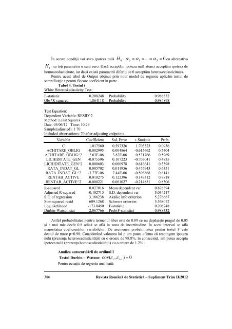
În aceste condiţii voi avea ipoteza nulă 0H : 0 1 ... 5 0cu alternativaH1 : nu toţi parametrii α sunt zero. Dacă acceptăm ipoteza nulă atunci acceptăm ipoteza dehomoscedasticitate, iar dacă există parametrii diferiţi de 0 acceptăm heteroscedasticitatea.Pentru acest tabel de Output obţinut prin noul model de regresie aplicăm testul desemnificaţie t pentru fiecare coeficient în parte.Tabel 4. Testul tWhite Heteroskedasticity Test:F-statistic 0.208248 Probability 0.988332Obs*R-squared 1.864118 Probability 0.984898Test Equation:Dependent Variable: RESID^2Method: Least SquaresDate: 05/06/12 Time: 10:29Sample(adjusted): 1 70Included observations: 70 after adjusting endpointsVariable Coefficient Std. Error t-Statistic Prob.C 1.017560 0.597326 1.703523 0.0936ACHITARE_OBLIG -0.002995 0.004864 -0.615662 0.5404ACHITARE_OBLIG^2 2.03E-06 3.82E-06 0.531766 0.5969LICHIDITATE_GEN -0.075596 0.107223 -0.705041 0.4835LICHIDITATE_GEN^2 0.000603 0.000978 0.616641 0.5398RATA_INDAT_GL 0.005702 0.011956 0.476943 0.6351RATA_INDAT_GL^2 -3.77E-06 7.44E-06 -0.506868 0.6141RENTAB_ACTIVE 0.018275 0.122396 0.149312 0.8818RENTAB_ACTIVE^2 -0.000221 0.001027 -0.214851 0.8306R-squared 0.027016 Mean dependent var 0.828394Adjusted R-squared -0.102715 S.D. dependent var 3.034217S.E. of regression 3.186238 Akaike info criterion 5.276667Sum squared resid 609.1268 Schwarz criterion 5.568072Log likelihood -173.0450 F-statistic 0.208248Durbin-Watson stat 2.067766 Prob(F-statistic) 0.988332Astfel probabilitatea pentru termenul liber este de 0.09 ce nu depăşeşte pragul de 0.05şi e mai mic decât 0.8 adică se află în zona de incertitudine. În acest interval se aflămajoritatea coeficienţilor variabilelor. De asemenea probabilitatea pentru testul F estedestul de mare p=0.98. Considerând valoarea lui p am putea afirma că respingem ipotezanulă (prezenţa heteroscedasticităţii) cu o eroare de 98.8%, în consecinţă, am putea acceptaipoteza nulă (prezenţa homoscedasticităţii) cu o eroare de 1.2% .Analiza autocorelării de ordinul ITestul Durbin – Watson: cov( ,1) 0Pentru ecuaţia de regresie analizată:t t386Revista Română de Statistică – Supliment Trim II/2012
Testul statistic DW foloseşte perechea de ipoteze:H0 : = 0 (ipoteza nulă); 1H : 0(ipoteza alternativă).Statistica DW este tabelată, valorile ei depinzând de nivelul de semnificaţieprecizat, de numărul de observaţii din eşantion şi de numărul variabilelor de influenţă dinmodelul de regresie. Aceasta, pentru un nivel de semnificaţie precizat, are două valoricritice ce se obţin din tabelele DW, d1 şi d2 .Regiunile de respingere a ipotezei nule sunt definite astfel:Dacă DW ( d 2,4 d2), nu există autocorelare;Dacă DW ( 0, d1)autocorelaţie pozitivă a erorilor;Dacă DW ( 4 d1,4)autocorelaţie negativă a erorilor;Dacă însă valoarea testului DW se află în intervalele rămase d , ) sau( 4 d2,4 d1)testul nu este concludent.( d 1 2În modelul analizat , statistica DW= 1.33. Pentru un prag de semnificaţie de 5%,un număr de 70 observaţii şi trei variabile de influenţă valorile tabelate ale statisticii sunt:d 1.49 iar d 1,74. Valoarea obţinută în model aparţine intervalului 0, d )12(1deci semanifestă fenomenul de autocorelare pozitivă a erorilor.În urma analizei datelor introduse în acest model de regresie multiplă, pentru maibune rezultate în privinţa homoscedasticităţii, autocorelării erorilor, sau normalităţiimodelului se pot introduce mai multe observaţii care să surprindă legăturile dintre ele.Aplicarea primului model pentru noul eşantion de firme a condus la următoarele rezultate:Dependent Variable: RENTAB_VENITMethod: Least SquaresDate: 05/06/12 Time: 10:47Sample: 1 30Included observations: 30RENTAB_VENIT=C(1)+C(2)*ACHITARE_OBLIG +C(3)*LICHIDITATE_GEN+C(4)* RATA_INDAT_GL +C(5)*RENTAB_ACTIVCoefficient Std. Error t-Statistic Prob.C(1) -26.02826 40.25845 -0.646529 0.5238C(2) -0.470880 0.455511 -1.033740 0.3112C(3) 0.120163 3.705339 0.032430 0.9744C(4) 0.426934 1.963538 0.217431 0.8296C(5) 0.263059 3.369060 0.078081 0.9384R-squared 0.044695 Mean dependent var -32.62267Adjusted R-squared -0.108153 S.D. dependent var 177.2346S.E. of regression 186.5728 Akaike info criterion 13.44653Sum squared resid 870235.2 Schwarz criterion 13.68006Log likelihood -196.6980 Durbin-Watson stat 2.0538993. ConcluziiŢinând seama de contextul economic actual, încercarea construirii unei funcții scorpentru previziunea falimentului întreprinderilor din România constituie o adevarataprovocare. Modelul econometric realizat este aplicat pe un eşantion de firme din diverseRevista Română de Statistică – Supliment Trim II/2012 387
Page 1 and 2: Forecasting <stron
Page 3 and 4: Jarque-Bera 891.7672 7758.419 10547
Page 5 and 6: lichiditate generală nu reprezint
Page 7 and 8: Testul Farrar-GlauberSe calculează
Page 9: ˆ este de medie nulă M 0, iar di

Forecasting the Bankruptcy Risk on the Example of Romanian ...

You also want an ePaper? Increase the reach of your titles

Delete template?

Save as template?