实验2 导数、微分、Taylor 公式2.1 实验目的理解导数、微分概念。理解 ...

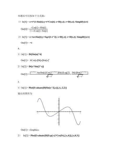
本 题 还 可 以 按 如 下 方 式 做 :
1)In[4]:= x=t*(1-Sin[t]);y=t*Cos[t]; s=D[y,t]; r=D[x,t]; Simplify[s/r]
− Cos[ t] + tSin[ t]
Out[4]=
− 1+ tCos[ t] + Sin[ t]
2)In[5]:= x=ArcSin[t];y=Sqrt[1-t^2]; s=D[y,t]; r=D[x,t]; Simplify[s/r]
Out[5]=
4.
1)In[1]:= Dt[Sin[u]^6]
Out[1]=
5
6Cos[ u]Dt[ u]Sin[ u ]
2)In[2]:= Dt[x*Sin[2^x]]
ArcSin[ t] ArcSin[ t] ArcSin[ t]
2 ArcSin[ t]Cos[2 ]D t[ t]Log[2] D t[ t]Sin[2 ]
Out[2]:=
+
2 2
1−t
1−t
5.
1)In[1]:= Plot[Evaluate[D[Sin[x^2],x]],{x,-2,2}]
输 出 的 图 形 为
3
2
1
-2 -1 1 2
-1
-2
-3
Out[1]= -Graphics-
2) In[2]:= Plot[Evaluate[D[Exp[-x]*Cos[5x],{x,4}]],{x,0,3}]