Forschung und wissenschaftliches Rechnen - Beiträge zum - GWDG

GWDG-Bericht Nr. 69 Kurt Kremer, Volker Macho (Hrsg.)
Forschung und
wissenschaftliches Rechnen
Beiträge zum
Heinz-Billing-Preis 2005
Gesellschaft für wissenschaftliche Datenverarbeitung mbH Göttingen

Forschung und
wissenschaftliches Rechnen

Titelbild:
Logo nach Paul Klee „Der Gelehrte“, Modifizierung durch I. Tarim,
Max-Planck-Institut für Psycholinguistik, Nijmegen.

GWDG-Bericht Nr. 69
Kurt Kremer, Volker Macho (Hrsg.)
Forschung und
wissenschaftliches Rechnen
Beiträge zum Heinz-Billing-Preis 2005
Gesellschaft für wissenschaftliche Datenverarbeitung
Göttingen
2006

Die Gesellschaft für wissenschaftliche Datenverarbeitung mbH Göttingen
ist eine gemeinsame Einrichtung der Max-Planck-Gesellschaft zur Förderung
der Wissenschaften e. V. und des Landes Niedersachsen. Die Max-
Planck-Gesellschaft hat diesen Bericht finanziell gefördert.
Redaktionelle Betreuung:
Volker Macho (Max-Planck-Institut fuer Polymerforschung, Mainz)
Satz:
Gesellschaft für wissenschaftliche Datenverarbeitung mbH Göttingen,
Am Faßberg, D-37077 Göttingen
Druck: klartext GmbH, D-37073 Göttingen, www.kopie.de
ISSN: 0176-2516

Inhalt
Vorwort
Kurt Kremer, Volker Macho ....................................................................... 1
Der Heinz-Billing-Preis 2005
Ausschreibung des Heinz-Billing-Preises 2005
zur Förderung des wissenschaftlichen Rechnens......................................... 5
Laudatio ...................................................................................................... 9
Patrick Jöckel, Rolf Sander:
The Modular Earth Submodel System (MESSy)....................................... 11
Nominiert für den Heinz-Billing-Preis 2005
Ewgenij Gawrilow, Michael Joswig:
Geometric Reasoning with polymake........................................................ 37
Christoph Wierling:
PyBioS - ein Modellierungs- und Simulationssystem für komplexe
biologische Prozesse ........................................................................................... 53

Weitere Beiträge für den Heinz-Billing-Preis 2005
Hans-Jörg Bibiko, Martin Haspelmath, Matthew S. Dreyer, David Gil,
Berard Comrie:
The Interactive Reference Tool for the
World Atlas of Language Structures.. ....................................................... 75
Beitrag zur Geschichte des wissenschaftlichen Rechnens
Aus den Erinnerungen von Prof. Dr. Heinz Billing................................... 85
Heinz Billing: In der Luftfahrtforschung (Auszug)............................... 87
Heinz Billing: Zurück und voran zur G1 bis G3......................................... 89
Anschriften der Autoren ..................................................................................... 105

Vorwort
Der vorliegende Band der Reihe „Forschung und wissenschaftliches
Rechnen“ enthält alle Beiträge, welche für den Heinz-Billing-Preis des
Jahres 2005 eingereicht wurden sowie zwei rückblickende Artikel von
Heinz Billing über die Anfänge des wissenschaftlichen Rechnens.
Der Hauptpreis ging in diesem Jahr an Patrick Jöckel und Rolf Sander
vom Max-Planck-Institut für Chemie für ihre Arbeit „The Modular Earth
Submodel System (MESSy) – A new approach towards Earth System
Modeling“. MESSy ermöglicht die Simulation von geophysikalischen Erdsystemmodellen,
in denen Prozesse sowohl in den Ozeanen, in der Luft und
im Wasser berücksichtigt werden und deren Rückkopplungsmechanismen
erfasst werden müssen. Mit MeSSy wird das Ziel verfolgt, ein umfassendes
Modellierungstool zu erstellen, welches sämtliche hierzu relevanten Submodell-Programme
miteinander verbinden kann. Geschrieben wurde das
Programm in Fortran-90.
Auf den zweiten Platz kam der Beitrag „Geometric Reasoning with
polymake“ von Ewgenij Gawrilow vom Institut für Mathematik der TU
Berlin sowie von Michael Joswig vom Fachbereich Mathematik der TU
Darmstadt. Polymake ist ein mathematisches Programmpaket zur Darstellung
von Polytopen und zur Berechnung ihrer Eigenschaften. Auch dieses
Programm ist in erster Linie ein Interface für eine Reihe anderer Programme,
welche Teilaspekte in Zusammenhang mit Polytopen behandeln.
Der dritte Platz ging an den Beitrag „PyBioS – ein Modellierungs- und
Simulationssystem für komplexe biologische Prozesse“ von Christoph
Wierling vom Max-Planck-Institut für Molekulare Genetik in Berlin, der
hiermit ein in Python geschriebenes, objektorientiertes und Web-basieren-
1

des Programmpaket vorstellt, welches für die Modellierung, Analyse und
Simulation von biologischen Reaktionsnetzwerken im Bereich der Systembiologie
Verwendung findet.
Zu guter Letzt möchten wir einige persönliche Erinnerungen von Prof.
Heinz Billing abdrucken, in denen er aus seiner Sicht die Entstehungsgeschichte
der so genannten „Göttinger Rechenmaschinen G1, G2 und G3“
sowie die Erfindung des Trommelspeichers beschreibt. Veröffentlicht sind
diese Erinnerungen in dem Buch „Die Vergangenheit der Zukunft“, herausgegeben
von Friedrich Genser und Johannes Hähnike. Der Nachdruck
erfolgt mit freundlicher Genehmigung des Autors und der Herausgeber.
Bedanken wollen wir uns ganz herzlich bei Günter Koch, GWDG, für
die Umsetzung der eingesandten Manuskripte in eine kompatible Druckvorlage.
Besonderer Dank gebührt Dr. Theo Plesser, der uns die Lebenserinnerungen
von Prof. Heinz Billing zusammen mit Abbildungen zur
Verfügung gestellt hat. Dank auch an die Pressestelle der MPG für die
Überlassung von Fotos.
Die Vergabe des Preises wäre ohne Sponsoren nicht möglich. Wir
danken der Firma IBM Deutschland, welche auch 2005 als Hauptsponsor
aufgetreten ist, für ihre großzügige Unterstützung.
Die hier abgedruckten Arbeiten sind ebenfalls im Internet unter der Adresse
www. billingpreis.mpg.de
zu finden.
Kurt Kremer, Volker Macho
2

Der Heinz-Billing-Preis 2005

Ausschreibung des Heinz-Billing-Preises 2005 zur
Förderung des wissenschaftlichen Rechnens
Im Jahre 1993 wurde zum ersten Mal der Heinz-Billing-Preis zur Förderung
des wissenschaftlichen Rechnens vergeben. Mit dem Preis sollen die Leistungen
derjenigen anerkannt werden, die in zeitintensiver und kreativer
Arbeit die notwendige Hard- und Software entwickeln, die heute für neue
Vorstöße in der Wissenschaft unverzichtbar sind.
Der Preis ist benannt nach Professor Heinz Billing, emeritiertes wissenschaftliches
Mitglied des Max-Planck-Institutes für Astrophysik und langjähriger
Vorsitzender des Beratenden Ausschusses für Rechenanlagen in der
Max-Planck-Gesellschaft. Professor Billing stand mit der Erfindung des
Trommelspeichers und dem Bau der Rechner G1, G2, G3 als Pionier der
elektronischen Datenverarbeitung am Beginn des wissenschaftlichen Rechnens.
Der Heinz-Billing-Preis zur Förderung des wissenschaftlichen Rechnens
steht unter dem Leitmotiv
„EDV als Werkzeug der Wissenschaft“.
Es können Arbeiten eingereicht werden, die beispielhaft dafür sind, wie
die EDV als methodisches Werkzeug Forschungsgebiete unterstützt oder
einen neuen Forschungsansatz ermöglicht hat.
5

Folgender Stichwortkatalog mag als Anstoß dienen:
– Implementierung von Algorithmen und Softwarebibliotheken
– Modellbildung und Computersimulation
– Gestaltung des Benutzerinterfaces
– EDV-gestützte Messverfahren
– Datenanalyse und Auswerteverfahren
– Visualisierung von Daten und Prozessen
Die eingereichten Arbeiten werden referiert und in der Buchreihe „Forschung
und wissenschaftliches Rechnen“ veröffentlicht. Die Jury wählt
einen Beitrag für den mit € 3000,- dotierten Heinz-Billing-Preis 2005 zur
Förderung des wissenschaftlichen Rechnens aus. Für die Beiträge auf den
Plätzen 2 und 3 werden jeweils 300,- Euro vergeben. Die Beiträge zum
Heinz-Billing-Preis, in deutscher oder englischer Sprache abgefasst, müssen
keine Originalarbeiten sein und sollten möglichst nicht mehr als fünfzehn
Seiten umfassen.
Da zur Bewertung eines Beitrages im Sinne des Heinz-Billing-Preises
neben der technischen EDV-Lösung insbesondere der Nutzen für das jeweilige
Forschungsgebiet herangezogen wird, sollte einer bereits publizierten
Arbeit eine kurze Ausführung zu diesem Aspekt beigefügt werden.
Der Heinz-Billing-Preis wird jährlich vergeben. Die Preisverleihung
findet anlässlich des 22. EDV-Benutzertreffens der Max-Planck-Institute
am 17. November 2005 in Göttingen statt.
Beiträge für den Heinz-Billing-Preis 2005 sind bis zum 30. Juni 2005
einzureichen.
Heinz-Billing-Preisträger
1993: Dr. Hans Thomas Janka, Dr. Ewald Müller, Dr. Maximilian Ruffert
Max-Planck-Institut für Astrophysik, Garching
Simulation turbulenter Konvektion in Supernova-Explosionen in
massereichen Sternen
1994: Dr. Rainer Goebel
Max-Planck-Institut für Hirnforschung, Frankfurt
- Neurolator - Ein Programm zur Simulation neuronaler Netzwerke
6

1995: Dr. Ralf Giering
Max-Planck-Institut für Meteorologie, Hamburg
AMC: Ein Werkzeug zum automatischen Differenzieren von
Fortran Programmen
1996: Dr. Klaus Heumann
Max-Planck-Institut für Biochemie, Martinsried
Systematische Analyse und Visualisierung kompletter Genome
am Beispiel von S. cerevisiae
1997: Dr. Florian Mueller
Max-Planck-Institut für molekulare Genetik, Berlin
ERNA-3D (Editor für RNA-Dreidimensional)
1998: Prof. Dr. Edward Seidel
Max-Planck-Institut für Gravitationsphysik, Albert-Einstein-
Institut, Potsdam
Technologies for Collaborative, Large Scale Simulation in Astrophysics
and a General Toolkit for solving PDEs in Science and
Engineering
1999: Alexander Pukhov
Max-Planck-Institut für Quantenoptik, Garching
High Performance 3D PIC Code VLPL:
Virtual Laser Plasma Lab
2000: Dr. Oliver Kohlbacher
Max-Planck-Institut für Informatik, Saarbrücken
BALL – A Framework for Rapid Application Development in
Molecular Modeling
2001: Dr. Jörg Haber
Max-Planck-Institut für Informatik, Saarbrücken
MEDUSA, ein Software-System zur Modellierung und Animation
von Gesichtern
2002: Daan Broeder, Hennie Brugman und Reiner Dirksmeyer
Max-Planck-Institut für Psycholinguistik, Nijmegen
NILE: Nijmegen Language Resource Environment
7

2003: Roland Chrobok, Sigurður F. Hafstein und Andreas Pottmeier
Universität Duisburg-Essen
OLSIM: A New Generation of Traffic Information Systems
2004: Markus Rampp, Thomas Soddemann
Rechenzentrum Garching der Max-Planck-Gesellschaft, Garching
A Work Flow Engine for Microbial Genome Research
2005: Patrick Jöckel, Rolf Sander
Max-Planck-Institut für Chemie, Mainz
The Modular Earth Submodel System (MESSy)
Das Kuratorium des Heinz-Billing-Preises
Prof. Dr. Heinz Billing
Emeritiertes Wissenschaftliches Mitglied des Max-Planck-Institut für
Astrophysik, Garching
Prof. Dr. Friedel Hossfeld
Forschungszentrum Jülich GmbH, Jülich
Prof. Dr. K. Ulrich Mayer
Max-Planck-Institut für Bildungsforschung, Berlin
Prof. Dr. Stefan Müller
Max-Planck-Institut für Mathematik in den Naturwissenschaften, Leipzig
Prof. Dr. Jürgen Renn
Max-Planck-Institut für Wissenschaftsgeschichte, Berlin
Prof. Dr. H. Wolfgang Spiess
Max-Planck-Institut für Polymerforschung, Mainz
8

Patrick Jöckel und Rolf Sander,
Max-Planck-Institut für Chemie, Mainz
erhalten den
Heinz-Billing-Preis 2005
zur Förderung
des wissenschaftlichen Rechnens
als Anerkennung für ihre Arbeit
The Modular Earth Submodel System (MESSy)
9

Laudatio
Der Heinz-Billing-Preis des Jahres 2005 wird für das Programmsystem The
Modular Earth Submodel System (MESSy) verliehen. Es handelt sich hierbei
um die Entwicklung einer modular strukturierten Softwareumgebung,
welche es gestattet, eine große Zahl von Modellen zur Beschreibung von
physikalischen und chemischen Prozessen der Atmosphäre zu integrieren.
Die enge raumzeitliche Kopplung luftchemischer und meteorologischer
Prozesse macht eine enge Verknüpfung der weltweit vorhandenen unterschiedlichen
Programmmodule erforderlich um eine effiziente Simulation
durchführen zu können.
Mit MESSy ist es nun möglich, Rückkopplungen zwischen den einzelnen
Prozessen zu untersuchen. Dies ist ein wichtiger Schritt zu einem geophysikalischen
Erdsystemmodell, in dem Prozesse sowohl im Ozean, an Land
und in der Luft in ihrer Wechselbeziehung effizient untersucht werden
können.
10
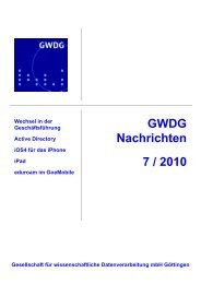
Verleihung des Heinz-Billing-Preises 2005 durch Prof. Kurt Kremer
an Patrick Jöckel (links) und Rolf Sander (rechts)

The Modular Earth Submodel System (MESSy) —
A new approach towards Earth System Modeling
Patrick Jöckel & Rolf Sander
Air Chemistry Department
Max-Planck Institute of Chemistry, Mainz, Germany
Abstract
The development of a comprehensive Earth System Model (ESM) to study the interactions between
chemical, physical, and biological processes requires coupling of the different domains
(land, ocean, atmosphere, ...). One strategy is to link existing domain-specific models with a
universal coupler, i.e. with an independent standalone program organizing the communication
between other programs. In many cases, however, a much simpler approach is more feasible. We
have developed the Modular Earth Submodel System (MESSy). It comprises (1) a modular interface
structure to connect submodels to a base model, (2) an extendable set of such submodels for
miscellaneous processes, and (3) a coding standard. In MESSy, data is exchanged between a base
model and several submodels within one comprehensive executable. The internal complexity of
the submodels is controllable in a transparent and user friendly way. This provides remarkable
new possibilities to study feedback mechanisms by two-way coupling. The vision is to ultimately
form a comprehensive ESM which includes a large set of submodels, and a base model which
contains only a central clock and runtime control. This goal can be reached stepwise, since each
process can be included independently. Starting from an existing model, process submodels can
be reimplemented according to the MESSy standard. This procedure guarantees the availability
of a state-of-the-art model for scientific applications at any time of the development. In principle,
MESSy can be implemented into any kind of model, either global or regional. So far, the MESSy
concept has been applied to the general circulation model ECHAM5 and a number of process
boxmodels.
11

Fig. 1: Process-oriented approach to establish an ESM. Each physical process is coded as a
modular entity connected via a standard interface to a common base model. The base model can
be for instance an atmosphere or ocean general circulation model (GCM), etc. At the final development
state, the base model contains hardly more than a central clock and the run control for
all modularized processes. All processes and the base model together form one comprehensive
executable. Data exchange between all processes is possible via the standard interface.
1 Introduction
The importance of environmental issues like climate change and the ozone
hole has received increased attention during the past decades. It has been
shown that the Earth (including the land, the oceans, and also the atmosphere)
is an extremely complex system. One powerful tool to investigate natural
cycles as well as potential anthropogenic effects is computer modeling. In
the early phase of the development most of the “historically grown” models
have been designed to address a few very specific scientific questions. The
codes have been continuously developed over decades, with steadily increasing
complexity. Additional processes were taken into consideration, so that
the computability was usually close to the limits of the available resources.
These historically grown model codes are now in a state associated with several
problems (see also Post and Votta, 2005):
– The code has mostly been developed by scientists, who are not necessarily
well-trained programmers. In principle every contribution follows its
developer’s unique style of programming. Coding conventions (e.g. http:
//www.meto.gov.uk/research/nwp/numerical/fortran90/f90_
standards.html) only help when strictly adhered to and when code reviews
are performed on a regular basis.
– The code has not been written to be easily extendable and adaptable to new
scientific questions.
– There has been little motivation for writing high quality code, since the
12

scientific aim had to be reached quickly. Well structured, readable code
has usually received low priority.
– Documentation lines within the code are often rare or absent.
– The code has been developed to run in a few specific configurations only,
e.g. in a particular vertical and horizontal resolution, and parameterizations
are resolution dependent.
– The code contains “hard-coded” statements, e.g. parameters implemented
explicitely as numerical values. Changes for sensitivity studies always require
recompilation.
– In many cases code developers (e.g. PhD students) are no longer available
for support and advice. If insurmountable obstacles occur, the code has to
be rewritten completely.
– Outdated computer languages (mostly Fortran77 or older) limit the full
exploitation of available hardware capacities. Therefore, the codes have
been “optimized” for specific hardware architectures, using non-standard,
vendor-specific language extensions. As a consequence, these codes are
not portable to other platforms.
– Compilers have been highly specific and error tolerant. Some even allowed
divisions by zero. Although this may seem an advantage, it must be
stressed that potentially serious code flaws are masked, which makes error
tracing extremely difficult.
The result is often a highly unreadable, undocumented “spaghetti-code”,
which inhibits an efficient further development. The same problems have to
be solved time and again. Transfering the code to a different environment
requires in many cases incommensurate efforts. Even worse than this development
aspect is the fact that those complex, non-transparent computer programs
elude more and more understanding, apart from a small, indispensable
group involved from the beginning.
2 Objectives
Any Earth System Model in general must fulfill several conditions to be consistent,
physically correct, flexible, sustainable, and extendable. To reach
these aims simultaneously, we define the following framework for the specific
implementation of MESSy:
– Modularity: Each specific process is coded as a separate, independent entity,
i.e. as a submodel, which can be switched on/off individually. This is
the consistent application of the operator splitting, which is implemented
in the models anyway.
– Standard interface: A so-called base model provides the framework to
which all submodels are connected. At the final state of development the
13

Fig. 2: Concepts of extending a GCM into a comprehensive ESM. The upper diagram shows that
in the “classical” way of development the code is handed over to the subsequent contributor
after a specific part has been finished. Parallel developments usually run into a dead end, since
different codes based on the same origin are usually no longer compatible. Furthermore, the
slowest contribution in the chain determines the overall progress. The lower diagram shows that
the new structure allows the development of all contributions in parallel, with the advantage
that the overall progress is NOT determined by the slowest contribution. At any time during
the development, a comprehensive state-of-the-art model is available (as indicated by the black
line).
base model should not contain more than a central clock for the time control
(time integration loop) and a flow control of the involved processes
(=submodels). This ultimate aim can be reached stepwise. For instance
one could start from an existing general circulation model (GCM) and
connect new processes via the standard interface. At the same time, it
is possible to modularize processes which are already part of the GCM,
and reconnect them via the standard interface. In many cases this requires
only a slightly modified reimplementation based on the existing code.
– Self-consistency: Each submodel is self-consistent, the submodel output is
uniquely defined by its input parameters, i.e., there are no interdependencies
to other submodels and/or the base model.
– Resolution independence: The submodel code is independent of the spatial
(grid) and temporal resolution (time step) of the base model. If applicable
and possible, the submodels are also independent of the dimensionality (0-
D (box), 1-D (column), 2-D, 3-D) and the horizontal (regional, global) and
vertical extent of the base model. Each process is coded for the smallest
applicable entity (box, column, column-vector, ...).
– Data flow: Exchange of data between the submodels and also between a
14

submodel and the base model is standardized.
– Soft-coding: The model code does not contain “hard-coded” specifications
which require a change of the code and recompilation after the model domain
or the temporal or spatial resolution is changed. A prominent example
is to use height or pressure for parameterizations of vertical profiles,
instead of level indices, as the latter have to be changed if the vertical resolution
of the base model is altered.
– Portability: All submodels are coded according to the language standard
of Fortran95 (ISO/IEC-1539-1). The code is free of hardware or vendorspecific
language extensions. In the rare cases where hardware specific
code is unavoidable (e.g. to circumvent compiler deficiencies), it is encapsulated
in preprocessor directives. MESSy allows for a flexible handling
on both, vector- and scalar- architectures. Compiler capabilities like automatic
vectorization (vector blocking) and inlining can be applied straightforwardly.
Last but not least, for an optimization, vector and scalar code
of the same process can coexist and switched on/off depending on the architecture
actually used.
– Multi-developer: The model system can be further developed by more than
one person at the same time without interference (see Fig. 2).
To meet the objectives described above, we have developed the Modular Earth
Submodel System (MESSy). It consists of:
1. a generalized interface structure for coupling processes coded as socalled
submodels to a so-called base model
2. an extendable set of processes coded as submodels
3. a coding standard
3 MESSy Interface Structure
The MESSy interface connects the submodels to the base model via a standard
interface. As a result, the complete model setup is organized in four
layers, as shown in Fig. 3:
1. The Base Model Layer (BML): At the final development state, this layer
comprises only a central time integration management and a run control
facility for the processes involved. In the transition state (at present) the
BML is the domain specific model with all modularized parts removed.
For instance, in case of an atmospheric model it can be a GCM.
2. The Base Model Interface Layer (BMIL), which comprises basically three
functionalities:
– The central submodel management interface allows the base model to
control (i.e. to switch and call) the submodels.
15

Fig. 3: The 4 layers of the MESSy interface structure (see Sect. 3 for a detailed description).
– The data transfer/export interface organizes the data transfer between
the submodels and the base model and between different submodels. It
is furthermore responsible for the output of results (export). Based on
the requirements of the model setup, the data can be classified according
to their use, e.g. as physical constants, as time varying physical fields,
and as tracers (i.e. chemical compounds).
– The data import interface is used for flexible (i.e. grid independent) import
of gridded initial and time dependent boundary conditions.
The BMIL therefore comprises the whole MESSy infrastructure which is
organized in so called generic submodels.
3. The Submodel Interface Layer (SMIL): This layer is a submodel-specific
interface, which collects all relevant information/data from the BMIL,
transfers them via parameter lists to the Submodel Core Layer (SMCL,
see below), calls the SMCL routines, and distributes the results from the
parameter lists back to the BMIL. Since this layer performs the data exchange
for the submodel, also the coupling between different submodels is
managed within this layer.
4. The Submodel Core Layer (SMCL): This layer comprises the self-consistent
core routines of a submodel (e.g. chemical integrations, physics, parameterizations,
diagnostic calculations), which are independent of the implementation
of the base model. Information exchange is solely performed
16

Fig. 4: Idealized flow chart of a typical MESSy setup (see Sect. 3 for details) consisting of three
submodels connected to the base model via the MESSy interface. The model simulation can be
subdivided into three phases: initialization phase, time integration phase, finalizing phase.
17

via parameter lists of the subroutines.
The user interface is implemented by using the Fortran95 namelist constructs,
and is connected to the three layers BMIL, SMIL, and SMCL.
The global switches to turn the submodels on and off are located in the
BMIL. These switches for all submodels are set by the run script.
Submodel-specific data initialization (e.g. initialization of chemical species
(=tracers)), and import of data within the time integration (e.g. temporally
changing boundary conditions) using the data import interface are handled
by the SMIL. Within the SMIL, also the coupling options from the user interface
are evaluated and applied, which control the coupling of the submodel to
the base model and to other submodels. For instance, the user has the choice
to select the submodel input from alternative sources, e.g. from results calculated
online by other submodels, or from data provided offline. Therefore,
this interface allows a straightforward implementation and management of
feedback mechanisms between various processes.
The control interface is located within the SMCL and manages the internal
complexity (and with this also the output) of the submodel. It comprises, for
instance, changeable parameter settings for the calculations, switches for the
choice of different parameterizations, etc.
A model simulation of a typical base model/MESSy setup can be subdivided
into three phases (initialization phase, time integration phase, finalizing
phase), as shown by the simplified flow chart in Fig. 4. The main control
(time integration and run control) is hosted by the base model, and therefore
the base model is also responsible for the flow of the three phases. After the
initialization of the base model, the MESSy infrastructure with the generic
submodels is initialized. At this stage the decision is made which submodels
are switched on/off.
Next, the active MESSy submodels are initialized sequentially. This initialization
is divided into two parts (not explicitly shown in Fig. 4). First, the
internal setup of all active submodels is initialized, and second the potential
coupling between all active submodels is performed. After the initialization
phase the time integration (time loop) starts, which is controlled by the base
model. All MESSy submodels are integrated sequentially according to the
operator splitting concept. At the end of the time integration, the MESSy
submodels and the MESSy infrastructure are finalized before the base model
terminates.
4 MESSy Submodels
Many submodels are now available within the MESSy system. Some of them
are completely new code whereas others have been adapted to MESSy based
18

Fig. 5: Overview of submodels currently available within MESSy
on pre-existing code. An overview of the submodels is shown in Fig. 5. In this
section we briefly present the submodels. For detailed information, please
contact the submodel maintainers. The submodel MECCA is explained in
more detail since it is the central part for the calculation of atmospheric chemistry.
Most submodels have been developed by us and by several colleagues
at our institute in Mainz. However, there are also several submodels resulting
from collaborations with other institutes. External contributions are from:
DLR: Deutsches Zentrum für Luft- und Raumfahrt, Institut für
Physik der Atmosphäre, Oberpfaffenhofen
ECMWF: European Centre for Medium-Range Weather Forecasts,
Reading, Great Britain
FFA: Ford Forschungszentrum, Aachen
JRC: Joint Research Centre, Ispra, Italy
LSCE: Laboratoire des Sciences du Climat et de l’Environnement,
France
MPI-BG: Max-Planck Institute for Biogeochemistry, Jena
MPI-MET: Max-Planck Institute for Meteorology, Hamburg
MSC: Meteorological Service of Canada
UNI-MZ: University of Mainz
UU: University of Utrecht, The Netherlands
19

4.1 AIRSEA
MAINTAINER: Andrea Pozzer
DESCRIPTION: This submodel calculates the emission (or deposition) of
various organic compounds. It is based on the two layer model for exchange
at the marine surface, with a pre-defined function for the sea water concentration
and an air concentration calculated in the model. In order to increase
the quality of the simulation, only the function for the concentrations in the
sea water has to be changed.
4.2 ATTILA
MAINTAINER: Patrick Jöckel, Michael Traub
ORIGINAL CODE: Christian Reithmeier (DLR), Volker Grewe (DLR),
Robert Sausen (DLR)
CONTRIBUTIONS: Volker Grewe (DLR), Gabriele Erhardt (DLR), Patrick
Jöckel
DESCRIPTION: The Lagrangian model ATTILA (Atmospheric Tracer Transport
In a Lagrangian Model) has been developed to treat the global-scale
transport of passive trace species in the atmosphere within the framework
of a general GCM. ATTILA runs online within a GCM and uses the GCMproduced
wind fields to advect the centroids of constant mass air parcels into
which the model atmosphere is divided. Each trace constituent is thereby represented
by a mixing ratio in each parcel. ATTILA contains state-of-the-art
parameterizations of convection and turbulent boundary layer transport.
4.3 CAM
MAINTAINER: Astrid Kerkweg
ORIGINAL CODE: Sunling Gong (MSC)
DESCRIPTION: The Canadian Aerosol Module (CAM) is a size-segregated
model of atmospheric aerosol processes for climate and air quality studies by
Gong et al. (2003). It is planned to integrate it into MESSy during the second
half of 2005.
4.4 CONVECT
MAINTAINER: Holger Tost
ORIGINAL CODE: M. Tiedtke (ECMWF), T. E. Nordeng (ECMWF)
DESCRIPTION: This submodel calculates the process of convection. It consists
of an interface to choose different convection schemes and the calculations
themselves. By now there are implemented the original ECHAM5 con-
20

vection routines with all three closures (Nordeng, Tiedtke, Hybrid) including
an update for positive definite tracers. Further schemes (ECMWF operational
scheme, Zhang-McFarlane-Hack, Bechtold) are currently being tested.
4.5 CVTRANS
MAINTAINER: Holger Tost
ORIGINAL CODE: Mark Lawrence
DESCRIPTION: The Convective Tracer Transport submodel calculates the
transport of tracers due to convection. It uses a monotonic, positive definite
and mass conserving algorithm following the bulk approach.
4.6 D14CO
MAINTAINER: Patrick Jöckel
DESCRIPTION: The cosmogenic isotope 14 C in its early state as 14 CO (carbon
monoxide) provides a natural atmospheric tracer, which is used for the
evaluation of the distribution and seasonality of the hydroxyl radical (OH)
and/or the strength, localization, and seasonality of the stratosphere to troposphere
exchange (STE) in 3-dimensional global atmospheric chemistry transport
models (CTMs) and general circulation models (GCMs).
4.7 DRADON
MAINTAINER: Patrick Jöckel
DESCRIPTION: This submodel uses 222 Rn as a tracer for diagnosing the
transport in and out of the boundary layer.
4.8 DRYDEP
MAINTAINER: Astrid Kerkweg
ORIGINAL CODE: Laurens Ganzeveld
CONTRIBUTIONS: Philip Stier (MPI-MET)
DESCRIPTION: This submodel calculates gas phase and and aerosol tracer
dry deposition according to the big leaf approach.
4.9 H2O
MAINTAINER: Christoph Brühl
ORIGINAL CODE: Christoph Brühl, Patrick Jöckel
DESCRIPTION: The H2O submodel defines H2O as a tracer, provides its
initialization in the stratosphere and the mesosphere from satellite data, and
controls the consistent feedback with specific humidity of the base model.
21

This submodel further accounts for the water vapor source of methane oxydation
in the stratosphere (and mesosphere), either by using the water vapor
tendency of a chemistry submodel (e.g. MECCA), or by using a satellite climatology
(UARS/HALOE) of methane together with monthly climatological
conversion rates.
4.10 JVAL
MAINTAINER: Rolf Sander
ORIGINAL CODE: Jochen Landgraf, Christoph Brühl, Wilford Zdunkowski
(UNI-MZ)
CONTRIBUTIONS: Patrick Jöckel
DESCRIPTION: This submodel is for fast online calculation of J-values (photolysis
rate coefficients) using cloud water content and cloudiness calculated
by the base model and/or climatological ozone and climatological aerosol.
A delta-twostream-method is used for 8 spectral intervals in UV and visible
together with precalculated effective cross-sections (sometimes temperature
and pressure dependent) for more than 50 tropospheric and stratospheric
species. If used for the mesosphere, also Ly-α radiation is included. Only the
photolysis rates for species present are calculated. Optionally, the UV-C solar
heating rates by ozone and oxygen are calculated.
4.11 LGTMIX
MAINTAINER: Patrick Jöckel
DESCRIPTION: Lagrangian Tracer Mixing in a semi-Eulerian approach.
4.12 LNOX
MAINTAINER: Patrick Jöckel
ORIGINAL CODE: Volker Grewe (DLR)
CONTRIBUTIONS: Laurens Ganzeveld, Holger Tost
DESCRIPTION: Parameterization of NOx (i.e. the nitrogen oxides NO and
NO2) produced by lightning
4.13 M7
MAINTAINER: Astrid Kerkweg
ORIGINAL CODE: Julian Wilson (JRC), Elisabetta Vignati (JRC)
CONTRIBUTIONS: Philip Stier (MPI-MET)
DESCRIPTION: M7 is a dynamical aerosol model that redistributes number
and mass between 7 modes and from the gas to the aerosol phase (for each
mode), by nucleation, condensation and coagulation.
22

Fig. 6: Selecting a chemical equation set and a numerical solver for KPP. See Sect. 4.15 for
further details.
4.14 MADE
MAINTAINER: Axel Lauer (DLR)
ORIGINAL CODE: Ingmar Ackermann et al. (FFA)
DESCRIPTION: The Modal Aerosol Dynamics model for Europe (MADE)
has been developed by Ackermann et al. (1998) as an extension to mesoscale
chemistry transport models to allow a more detailed treatment of aerosol effects
in these models. In MADE, the particle size distribution of the aerosol
is represented by overlapping lognormal modes. Sources for aerosol particles
are modelled through nucleation and emission. Coagulation, condensation,
and deposition are considered as processes modifying the aerosol population
in the atmosphere. The adaptation of MADE to the MESSy standard is currently
under construction.
4.15 MECCA
MAINTAINER: Rolf Sander, Astrid Kerkweg
CONTRIBUTIONS: Rolf von Kuhlmann, Benedikt Steil, Roland von Glasow
DESCRIPTION: The Module Efficiently Calculating the Chemistry of the
Atmosphere (MECCA) by Sander et al. (2005) calculates tropospheric and
stratospheric chemistry. Aerosol Chemistry in the marine boundary layer is
also included. The main features of MECCA are:
23

Chemical flexibility: The chemical mechanism contains a large number of
reactions from which the user can select a custom-designed subset. It is
easy to adjust the mechanism, e.g. according to the latest kinetics insights.
Numerical flexibility: The numerical integration method can be chosen according
to individual requirements of the stiff set of differential equations
(efficiency, stability, accuracy, precision).
In the current version of MECCA, five previously published chemical mechanisms
have been combined and updated. Tropospheric hydrocarbon chemistry
is adopted from the MATCH model by von Kuhlmann et al. (2003). The
chemistry of the stratosphere is based on MAECHAM4/CHEM by Steil et al.
(1998) and the Mainz Chemical Box Model (Meilinger, 2000). Tropospheric
halogen chemistry is taken from MOCCA by Sander and Crutzen (1996) and
from MISTRA by von Glasow et al. (2002). The current mechanism contains
116 species and 295 reactions in the gas phase, and 91 species and 258
reactions in the aqueous phase. The rate coefficients are updated according
to Sander et al. (2003), Atkinson et al. (2004), and other references. A detailed
listing of reactions, rate coefficients, and their references can be found
in the electronic supplement of Sander et al. (2005). It is both possible and
desirable to add reactions to the mechanism in the near future. However, for
computational efficiency, it is normally not required to integrate the whole
mechanism. Therefore we have implemented a method by which the user can
easily create a custom-made chemical mechanism. Each reaction has several
labels to categorize it. For example, the labels Tr and St indicate reactions relevant
in the troposphere and the stratosphere, respectively. These labels are
not mutually exclusive. Many reactions need to be considered for both layers.
There are also labels for the phase in which they occur (gas or aqueous phase)
and for the elements that they contain (e.g. Cl, Br, andI for reactions of the
halogen species). It is also possible to create new labels for specific purposes.
For example, all reactions with the label Mbl are part of a reduced mechanism
for the marine boundary layer. Using a Boolean expression based on
these labels, it is possible to create custom-made subsets of the comprehensive
mechanism. The main advantage of maintaining a single comprehensive
mechanism is that new reactions and updates of rate coefficients need to be
included only once so that they are immediately available for all subsets.
Once a subset of the full mechanism has been selected as described above,
the kinetic preprocessor (KPP) software (Sandu and Sander, manuscript in
preparation, 2005) is used to transform the chemical equations into Fortran95
code. From a numerical point of view, atmospheric chemistry is a challenge
due to the coexistence of very stable (e.g. CH4) and very reactive species,
e.g. O( 1 D). To overcome the stiffness issue, associated with the large range
of timescales within a single set of differential equations, robust numerical
solvers are necessary. KPP provides several solvers with either manual or
24

automatic time step control. Although computationally more demanding, the
latter are best suited for the most difficult stiffness problems e.g. associated
with multiphase chemistry. For each individual application, it is necessary to
balance the advantages and disadvantages regarding efficiency, stability, accuracy,
and precision. We found that for most of our chemical mechanisms,
the Rosenbrock solvers of 2nd or 3rd order (ros2 and ros3) work best. However,
we stress that it may be necessary to test other solvers as well (e.g.
radau5) to achieve the best performance for a given set of equations. Fortunately,
switching between solvers is easy with KPP and does not require
any reprogramming of the chemistry scheme. The selection of a chemical
equation set and a numerical solver is shown in Fig. 6.
4.16 OFFLEM
MAINTAINER: Patrick Jöckel
DESCRIPTION: This submodel reads input data from files for two-dimensional
emission fluxes (i.e. surface emissions in molecules/(m 2 s)) and threedimensional
emission fluxes (aircraft emissions in molecules/(m 3 s)) and updates
the tracer tendencies (gridpoint- and Lagrangian) accordingly.
4.17 ONLEM
MAINTAINER: Astrid Kerkweg
CONTRIBUTIONS: Yves Balkanski (LSCE), Ina Tegen (MPI-BG), Philip
Stier (MPI-MET), Sylvia Kloster (MPI-MET), Laurens Ganzeveld, Michael
Schulz (LSCE)
DESCRIPTION: This submodel calculates two-dimensional emission fluxes
for gas-phase tracers (i.e. surface emissions in molecules/(m 2 s)) and updates
the tracer tendencies accordingly. In addition, aerosol source functions are
calculated.
4.18 PSC
MAINTAINER: Joachim Buchholz
ORIGINAL CODE: Ken Carslaw, Stefanie Meilinger, Joachim Buchholz
DESCRIPTION: The Polar Stratospheric Cloud (PSC) submodel simulates
micro-physical processes that lead to the formation of super-cooled ternary
solutions (STS), nitric acid trihydrate (NAT), and ice particles in the polar
stratosphere as well as heterogeneous chemical reactions of halogens and
dinitrogen pentoxide on liquid and solid aerosol particles. Denitrification and
dehydration due to sedimenting solid PSC particles are calculated for each
grid box depending on particle size, pressure and temperature.
25

4.19 PTRAC
MAINTAINER: Patrick Jöckel
DESCRIPTION: This submodel uses user-defined initialized passive tracers
to test mass conservation, monotonicity, and positive definiteness of Eulerian
and Lagrangian advection algorithms.
4.20 QBO
MAINTAINER: Maarten van Aalst (UU)
ORIGINAL CODE: Marco Giorgetta (MPI-MET)
CONTRIBUTIONS: Patrick Jöckel
DESCRIPTION: This submodel is for assimilation of QBO zonal wind observations.
4.21 SCAV
MAINTAINER: Holger Tost
DESCRIPTION: The Scavenging submodel simulates the processes of wet
deposition and liquid phase chemistry in precipitation fluxes. It considers
gas-phase and aerosol species in large-scale as well as in convective clouds
and precipitation events.
4.22 SCOUT
MAINTAINER: Patrick Jöckel
DESCRIPTION: The submodel ’Selectable Column Output’ generates highfrequency
output of user-defined fields at arbitrary locations.
4.23 SEDI
MAINTAINER: Astrid Kerkweg
DESCRIPTION: This submodel calculates sedimentation of aerosol particles
and their components.
4.24 TNUDGE
MAINTAINER: Patrick Jöckel
DESCRIPTION: The submodel ’Tracer Nudging’ is used for nudging userdefined
tracers with arbitrary user-defined data sets.
26

4.25 TRACER
MAINTAINER: Patrick Jöckel
DESCRIPTION: Tracers are chemical species that are transported in the atmosphere
according to the model-calculated wind fields and other processes.
This generic submodel handles the data and metadata associated with tracers.
It also provides the facility to transport user-defined subsets of tracers
together inside a tracer family.
4.26 TROPOP
MAINTAINER: Patrick Jöckel
CONTRIBUTIONS: Michael Traub, Benedikt Steil
DESCRIPTION: This submodel calculates the position of the tropopause.
Two definitions are implemented: A potential vorticity iso-surface (usually
used at high latitudes) and the thermal tropopause according to the definition
of the World Meteorological Organization (WMO), usually used in the
tropics).
4.27 VISO
MAINTAINER: Patrick Jöckel
DESCRIPTION: ’Values on horizontal (Iso)-Surfaces’ is a submodel for userdefined
definition of horizontal iso-surfaces and output of user-defined data
on horizontal surfaces (tropopause, boundary layer height, iso-surfaces, ...).
5 MESSy Coding Standard
As stated above, strict adherence to a coding standard is an absolutely necessary
prerequisite for the maintenance of a very comprehensive Earth System
Models. The full MESSy coding standard has been published in Jöckel et al.
(2005). Here, we only briefly summarize the main points.
For the implementation of the MESSy interface, all changes to the base
model are coded with “keyhole surgery”. This means that changes to the base
model are only allowed if they are really needed, and if they are as small as
possible. Changes to the base model code are encapsulated in preprocessor
directives:
#ifndef MESSY
# else
27

#endif
Likewise, additional code is encapsulated as
#ifdef MESSY
#endif
Overall, code development obeys the following rules:
– Each process is represented by a separate submodel.
– Every submodel has a unique name.
– A submodel is per default switched OFF and does nothing unless it has
been switched on (USE_=T) by the user via a unique namelist
switch in the run script xmessy.
– Several submodels for the same process (e.g. different parameterizations)
can coexist.
– Each submodel consists of two modules (two layers):
1. submodel core layer (SMCL): A completely self-consistent, base model
independent Fortran95 core-module to/from which all required quantities
are passed via parameters of its subroutines. Self-consistent means
that there are neither direct connections to the base model, nor to other
submodels. The core-module provides PUBLIC subroutines which are
called by the interface-module, and PRIVATE subroutines which are
called internally.
2. submodel interface layer (SMIL): An interface-module which organizes
the calls and the data exchange between submodel and base model. Data
from the base model is preferably accessed via the generic submodel
SMIL “main_data”. The interface module provides a set of PUBLIC
subroutines which constitute the main entry-points called from the
MESSy central submodel control interface.
– The core module must be written to run as the smallest possible entity
(e.g. box, column, column-vector (2-D), global) on one CPU in a parallel
environment (e.g. MPI). Therefore, STOP-statements must be omitted and
replaced by a status flag (INTENT(OUT)) which is 0, if no error occurs.
Inthesameway,WRITE- andPRINT-statements must only occur in the
part of the code which is exclusively executed by a dedicated I/O processor.
This is controlled in the SMIL.
– Data transfer between submodels is performed exclusively within the interface
layer. Direct USE-statements to other submodels are not allowed.
– The internal application flow of a submodel is controlled by switches and
parameters in the CTRL-namelist; coupling to the base model and/or other
submodels is defined via switches and parameters in the CPL-namelist.
– The filename of each MESSy file identifies submodel, layer, and type:
messy_[_]
28

[_mem][_].f90 where [...] means “optional”,
means a specific name, mem indicates “memory”-files, and the
interface layer modules. Each Fortran module must have the same name
as the file it resides in, however with the suffix .f90 removed.
– If the complexity of a submodel requires separation into two or more
files per layer (core or interface), shared type-, variable- and parameterdeclarations
can be located in *_mem.f90 files (or *_mem_.f90
files, respectively) which can be USEd by the submodel files within the
respective layer. These memory-modules must be used by more than 1
file within the relevant layer, and must not contain any subroutine and/or
function.
– MESSy-submodels are independent of the specific base model resolution
in space and time. If this is not possible (e.g., for specific parameterizations)
or not yet implemented, the submodel needs to terminate the model
in a controlled way (via the status flag), if the required resolution has not
been chosen by the user.
– A submodel can host sub-submodels, e.g. for different various parameterizations,
sub-processes, etc.
– The smallest entities of a submodel, i.e. the subroutines and functions,
must be as self-consistent as possible according to:
· USE-statements specific for a certain subroutine or function must be
placed where the USEd objects are needed, not into the declaration section
of the module.
· IMPLICIT NONE is used for all modules, subroutines and functions.
· If a function or subroutine provides an internal consistency check, the
result must be returned via an INTEGER parameter (status flag), which
is 0, if no error occurs, and identifies the problem otherwise.
– PRIVATE must be the default for every module, with the exception of
memory-files. The PUBLIC attribute must explicitely used only for those
subroutines, functions, and variables that must be available outside of the
module.
– Variables must be defined (not only declared!). The best way to define a
variable is within its declaration line, e.g.:
INTEGER :: n = 0
– Pointers need to be nullified, otherwise, the pointer’s association status
will be initially undefined. Pointers with undefined association status tend
to cause trouble. According to the Fortran95 standard even the test of the
association status with the intrinsic function ASSOCIATED is not allowed.
Nullification of a pointer is preferably performed at the declaration
REAL, DIMENSION(:,:), POINTER :: &
ptr => NULL()
or at the beginning of the instruction block with
29

Fig. 7: MESSy can be used for the whole range from box models to global GCMs. See Sect. 6 for
details.
NULLIFY(ptr)
– Wherever possible, ELEMENTAL and/or PURE functions and subroutines
must be used.
– Numeric precision is controlled within the code by specifying the KIND
parameters. Compiler switches to select the numeric precision (e.g. “-r8”)
must be avoided.
– Since the dependencies for the build-process are generated automatically,
obsolete, backup- or test-files must not have the suffix .f90. Instead, they
must be renamed to *.f90-bak or something similar.
– Any USE command must be combined with an ONLY statement. This
makes it easier to locate the origin of non-local variables. (Exception: A
MESSy-core module may be used without ONLY by the respective MESSyinterface
module.)
6 Application
A box model often contains a highly complex mechanism. It is integrated
for a relatively short simulation time only (e.g. days or weeks). A GCM
simulation usually covers several years, but contains a much less complex
description of individual atmospheric processes. The MESSy system can be
used for the whole range from box models to GCMs (see Fig. 7). Although
most submodels are mainly written for the inclusion into larger regional and
global models (e.g. GCMs), the MESSy structure supports and also encourages
their connection to a box model, whereby “box model” is defined here
as the smallest meaningful entity for a certain process which is running independently
of the comprehensive ESM. We have applied the MESSy structure
to miscellaneous box models.
30

Fig. 8: A MESSy submodel (here MECCA is shown as an example for atmospheric chemistry
integrations) can be coupled to several base models without modifications. The submodel core
layer, as indicated by the separated box, is always independent of the base model. Note that at
the final development state of MESSy, also the second layer from below (submodel interface layer
(SMIL), pale yellow area) is likewise independent of the base model, since it solely makes use of
the MESSy infrastructure, for instance the data transfer and export interface. Last but not least,
the base model dependence of the second layer from above (base model interface layer, BMIL)
is minimized by extensive usage of the MESSy infrastructure. Only well defined connections (as
indicated by arrows between BML and BMIL in Figure 3) are required.
As an example, Fig. 8 shows how the atmospheric chemistry submodel
MECCA can be connected to either a simple box model, or to a complex
GCM. Note that exactly the same files of the chemistry submodel are used in
both cases. Therefore, box models are an ideal environment for debugging
and evaluating a submodel. While developing the submodel, it can be tested
in fast box model runs without the need for expensive global model simulations.
Once the submodel performs well, it can directly be included into the
GCM without any further changes.
The MESSy interface has also been successfully connected to the general
circulation model ECHAM5 (Roeckner et al., The atmospheric general circulation
model ECHAM 5. PART I: Model description, MPI-Report, 349,
2003), thus extending it into a fully coupled chemistry-climate model. This
provides exciting new possibilities to study feedback mechanisms. Examples
include stratosphere-troposphere coupling, atmosphere-biosphere interactions,
multi-component aerosol processes, and chemistry-climate interactions.
MESSy also provides an important tool for model intercomparisons and
process studies. As an example, aerosol-climate interactions could be investigated
in two model runs in which two different aerosol submodels are
31

switched on. For processes without feedbacks to the base model, it is even
possible to run several submodels for the same process simultaneously. For
example, the results of two photolysis schemes could be compared while ensuring
that they both receive exactly the same meteorological and physical
input from the GCM.
7 Conclusions
The transition from General Circulation Models (GCMs) to Earth System
Models (ESMs) requires the development of new software technologies and
a new software management, since the rapidly increasing model complexity
needs a transparent control. The Modular Earth Submodel System (MESSy)
provides a generalized interface structure, which allows unique new possibilities
to study feedback mechanisms between various bio-geo-chemical processes.
Strict compliance with the ISO-Fortran95 standard makes it highly
portable to different hardware platforms. The modularization allows for uncomplicated
connection to various base models, as well as the co-existence
of different algorithms and parameterizations for the same process, e.g. for
testing purposes, sensitivity studies, or process studies. The coding standard
provides a multi-developer environment, and the flexibility enables a large
number of applications with different foci in many research topics referring
to a wide range of temporal and spatial scales.
MESSy is an activity that is open to the scientific community following
the “open source” philosophy. We encourage collaborations with colleague
modelers, and aim to efficiently achieve improvements. The code is available
at no charge. For details, we refer to Jöckel et al. (2005) and our web-site
http://www.messy-interface.org.
Additional submodels and other contributions from the modeling community
will be highly appreciated. We encourage modelers to adapt their code
according to the MESSy-standard and we look forward to receiving interesting
contributions from the geosciences modeling community.
References
Ackermann, I. J., Hass, H., Memmesheimer, M., Ebel, A., Binkowski, F. S., and Shankar,
U.: Modal aerosol dynamics model for Europe: development and first applications, Atmos.
Environ., 32, 2981–2999, 1998.
Atkinson, R., Baulch, D. L., Cox, R. A., Crowley, J. N., Hampson, R. F., Hynes, R. G., Jenkin,
M. E., Rossi, M. J., and Troe, J.: Evaluated kinetic and photochemical data for atmospheric
chemistry: Volume I – gas phase reactions of Ox, HOx, NOx and SOx species, Atmos. Chem.
Phys., 4, 1461–1738, 2004.
Gong, S. L., Barrie, L. A., Blanchet, J.-P., von Salzen, K., Lohmann, U., Lesins, G., Spacek,
L., Zhang, L. M., Girard, E., Lin, H., Leaitch, R., Leighton, H., Chylek, P., and Huang, P.:
Canadian Aerosol Module: A size-segregated simulation of atmospheric aerosol processes for
32

climate and air quality models 1. Module development, J. Geophys. Res., 108D, doi:10.1029/
2001JD002002, 2003.
Jöckel, P., Sander, R., Kerkweg, A., Tost, H., and Lelieveld, J.: Technical Note: The Modular
Earth Submodel System (MESSy) – a new approach towards Earth System Modeling, Atmos.
Chem. Phys., 5, 433–444, 2005.
Meilinger, S. K.: Heterogeneous Chemistry in the Tropopause Region: Impact of Aircraft
Emissions, Ph.D. thesis, ETH Zürich, Switzerland, http://www.mpch-mainz.mpg.de/
~smeili/diss/diss_new.ps.gz, 2000.
Post, D. E. and Votta, L. G.: Computational science demands a new paradigm, Physics Today,
pp. 35–41, 2005.
Sander, R. and Crutzen, P. J.: Model study indicating halogen activation and ozone destruction
in polluted air masses transported to the sea, J. Geophys. Res., 101D, 9121–9138, 1996.
Sander, R., Kerkweg, A., Jöckel, P., and Lelieveld, J.: Technical Note: The new comprehensive
atmospheric chemistry module MECCA, Atmos. Chem. Phys., 5, 445–450, 2005.
Sander, S. P., Finlayson-Pitts, B. J., Friedl, R. R., Golden, D. M., Huie, R. E., Kolb, C. E.,
Kurylo, M. J., Molina, M. J., Moortgat, G. K., Orkin, V. L., and Ravishankara, A. R.: Chemical
Kinetics and Photochemical Data for Use in Atmospheric Studies, Evaluation Number 14, JPL
Publication 02-25, Jet Propulsion Laboratory, Pasadena, CA, 2003.
Steil, B., Dameris, M., Brühl, C., Crutzen, P. J., Grewe, V., Ponater, M., and Sausen, R.:
Development of a chemistry module for GCMs: First results of a multiannual integration, Ann.
Geophys., 16, 205–228, 1998.
von Glasow, R., Sander, R., Bott, A., and Crutzen, P. J.: Modeling halogen chemistry
in the marine boundary layer, 1. Cloud-free MBL, J. Geophys. Res., 107D, 4341, doi:
10.1029/2001JD000942, 2002.
von Kuhlmann, R., Lawrence, M. G., Crutzen, P. J., and Rasch, P. J.: A model for studies
of tropospheric ozone and nonmethane hydrocarbons: Model description and ozone results, J.
Geophys. Res., 108D, doi:10.1029/2002JD002893, 2003.
33

Nominiert für den Heinz-Billing-Preis 2005

Geometric Reasoning with polymake
Ewgenij Gawrilow
Institut für Mathematik, MA 6-1, TU Berlin
Michael Joswig
Fachbereich Mathematik, AG 7, TU Darmstadt
Abstract
The mathematical software system polymake provides a wide range of functions for convex
polytopes, simplicial complexes, and other objects. A large part of this paper is dedicated to a
tutorial which exemplifies the usage. Later sections include a survey of research results obtained
with the help of polymake so far and a short description of the technical background.
1 Introduction
The computer has been described as the mathematical machine. Therefore, it
is nothing but natural to let the computer meet challenges in the area where
its roots are: mathematics. In fact, the last two decades of the 20th century
saw the ever faster evolution of many mathematical software systems, general
and specialized. Clearly, there are areas of mathematics which are more apt
to such an approach than others, but today there is none which the computer
could not contribute to.
In particular, polytope theory which lies in between applied fields, such
as optimization, and more pure mathematics, including commutative algebra
and toric algebraic geometry, invites to write software. When the polymake
37

project started in 1996, there were already a number of systems around which
could deal with polytopes in one way or another, e.g., convex hull codes such
as cdd [10], lrs [3], porta [7], and qhull [6], but also visualization classics
like Geomview [1]. The basic idea to polymake was —and still is—
to make interfaces between any of these programs and to continue building
further on top of the combined functionality. At the same time the gory technical
details which help to accomplish such a thing should be entirely hidden
from the user who does not want to know about it. On the outside polymake
behaves somewhat similar to an expert system for polytopes: The user once
describes a polytope in one of several natural ways and afterwards he or she
can issue requests to the system to compute derived properties. In particular,
there is no need to program in order to work with the system. On the other
hand, for those who do want to program in order to extend the functionality
even further, polymake offers a variety of ways to do so.
The modular design later, since version 2.0, allowed polymake to treat
other mathematical objects in the same way, in particular, finite simplicial
complexes For the sake of brevity, however, this text only covers polymake’s
main application which is all about polytopes.
We explain the organization of the text. It begins with a quite long tutorial
which should give an idea of how the system can be used. The examples are
deliberately chosen to be small enough that it is possible to verify all claims
while reading. What follows is an overall description of the key algorithms
and methods which are available in the current version 2.1. The subsequent
Section 6 contains several brief paragraphs dedicated to research in mathematics
that was facilitated by polymake.
Previous reports on the polymake system include the two papers [11,
12]; by now they are partially outdated. polymake is open source software
which can be downloaded from http://www.math.tu-berlin.de/
polymake for free.
2 What Are Polytopes and Why Are They Interesting?
A polytope is defined as the convex hull of finitely many points in Euclidean
space. If one thinks of a given finite number of points as very small balls,
with fixed positions, then wrapping up all these points as tightly as possible
into one large “gift” yields the polytope generated by the points. In fact,
there are algorithms which follow up this gift-wrapping idea quite closely in
order to obtain a so-called outer description of the polytope. A 2-dimensional
polytope is just a planar convex polygon.
Polytopes are objects which already fascinated the ancient Greeks. They
were particularly interested in highly symmetric 3-dimensional polytopes.
38

Fig. 1: One Platonic and Two Archimedean Solids: icosahedron, snub cube, and truncated
icosahedron (soccer ball).
Today polytopes most frequently show up as the sets of admissible points
of linear programs. Linear programming is about optimizing a linear objective
function over a domain which is defined by linear inequalities. If this
domain is bounded then it is a polytope; otherwise it is called an unbounded
polyhedron. Linear programs are at the heart of many optimization problems
in scientific, technical, and economic applications.
But also within mathematics polytopes play their role. For instance, in the
seventies of the twentieth century it became apparent that they are strong ties
between algebraic geometry and the theory of polytopes via the concept of a
toric variety. For this and other reasons in the sequel it became interesting to
investigate metric and combinatorial properties of polytopes in much gerater
depth than previously; see the monograph of Ewald [9]. The purpose of the
polymake system is to facilitate this kind of research.
3 A polymake Tutorial
This tutorial tries to give a first idea about polymake’s features by taking a
look at a few small examples. We focus on computations with convex polytopes.
For definitions, more explanations, and pointers to the literature see
the subsequent Section 4.
The text contains commands to be given to the polymake system (preceded
by a ’>’) along with the output. As the environment a standard UNIX
shell, such as bash, is assumed. Commands and output are displayed in
typewriter type.
Most of the images shown are produced via polymake’s interface to
JavaView [22] which is fully interactive.
39

3.1 A very simple example: the 3-cube
Suppose you have a finite set of points in the Euclidean space Ê d . Their
convex hull is a polytope P . Now you want to know how many facets P has.
As mentioned previously, polytopes can also be described as the set of points
satisfying a finite number of linear inequalities. The facets correspond to the
(uniquely determined) set of non-redundant linear inequalities.
As an example let the set S consist of the points (0, 0, 0), (0, 0, 1), (0, 1, 0),
(0, 1, 1), (1, 0, 0), (1, 0, 1), (1, 1, 0), (1, 1, 1) in R 3 . Clearly, S is the set of
vertices of a cube; and its facets are the six quadrangular faces. Employing
your favorite word processor produce an ASCII text file, say cube.poly,
containing precisely the following information.
POINTS
1 0 0 0
1 0 0 1
1 0 1 0
1 0 1 1
1 1 0 0
1 1 0 1
1 1 1 0
1 1 1 1
We have the keyword POINTS followed by eight lines, where each line
contains the coordinates of one point. The coordinates in Ê 3 are preceded
by an additional 1 in the first column; this is due to the fact that polymake
works with homogeneous coordinates. The solution of the initial problem can
now be performed by polymake as follows. Additionally, we want to know
whether P is simple, that is, whether each vertex is contained in exactly 3
facets (since dim P =3).
> polymake cube.poly N_FACETS SIMPLE
While polymake is searching for the answer, let us recall what polymake
has to do in order to obtain the solution. It has to compute the convex hull
of the given point set in terms of an explicit list of the facet describing inequalities.
Then they have to be counted, which is, of course, the easy part.
Nonetheless, polymake decides on its own what has to be done, before the
final —admittedly trivial— task can be performed. Checking simplicity requires
to look at the vertex facet incidences. In the meantime, polymake is
done. Here is the answer.
N_FACETS
6
SIMPLE
1
40

Simplicity is a boolean property. So the answer is either “yes” or “no”,
encoded as 1 or 0, respectively. The output says that P is, indeed, simple.
Asamatteroffact,polymake knows quite a bit about standard constructions
of polytopes. So you do have to type in your 3-cube example. You can
use the following command instead. The trailing argument 0 indicates a cube
with 0/1-coordinates.
> cube cube.poly 3 0
3.2 Visualizing a Random Polytope
But let us now try something else. How does a typical polytope look like?
To be more precise: Show me an instance of the convex hull of 20 randomly
distributed points on the unit sphere in R3 . This requires one command to
produce a polymake description of such a polytope and a second one to
trigger the visualization. Again there is an implicit convex hull computation
going on behind the scenes. On the way a complete combinatorial description
of the polytope is obtained.
> rand_sphere random.poly 3 20
> polymake random.poly VISUAL
polymake’s standard tool for interactive visualization is JavaView by
Polthier and others [22] For instance, it allows you to rotate or zoom into your
polytope. Here is a sequence of snapshots.
Fig. 2: Interactive visualization of a random polytope with JavaView: Three snapshots.
3.3 Linear programming
Polytopes most naturally appear as sets of feasible solutions of linear programs.
Consider the following example.
A linear inequality a0 + a1x1 + ...adxd ≥ 0 is encoded as the inward
pointing normal vector to the corresponding affine hyperplane (of suitable
length). This is what polymake uses: the former inequality is represented
as the vector (a0,a1,...,ad). Our linear program in polymake’s format
41

Maximize
x1 + x2 + x3
subject to
0 ≤ x1,x2,x3 ≤ 1
x1 + x2 + x3 ≤ 5/2
x1 − 17x2 ≤ 8
Fig. 3: Small linear program and a visualization.
looks as given below. Note that we do not decide beforehand, whether we
want to minimize or maximize.
LINEAR_OBJECTIVE
0 1 1 1
INEQUALITIES
0 1 0 0
0 0 1 0
0 0 0 1
1 -1 0 0
1 0 -1 0
1 0 0 -1
5/2 -1 -1 -1
8 -1 17 0
People working in optimization usually prefer other file formats (such as
CPLEX’s LP file format), where it is also possible to keep the names of the
variables. polymake is aware of this. LP format files can be converted by
calling the command lp2poly.
It is not difficult to determine the polytope forming the solution space.
Assume the file linear_program.poly contains the description given
above.
> polymake linear_program.poly MAXIMAL_VALUE
MAXIMAL_VALUE
5/2
This is the kind of behavior one would expect from a linear solver. Of
course, usually it is also interesting to obtain a point attaining the maximum.
And, in fact, polymake calls cdd’s implementation of the Simplex Method
(with exact rational arithmetic). With polymake you can go one step further.
It visualizes for you the polytope with directed edges. Instead of relying
42
4
5
6
8
9
2
3
7
1
0

on the interactive JavaView visualization this time we produce postscript
output directly; see Figure 3.
> polymake linear_program.poly postscript \
"VISUAL_GRAPH->DIRECTED_GRAPH->VERTEX_COLORS"
The directed edges (whose orientation is induced by the given linear objective
function) are drawn as arrows. The colors of the vertices indicate the
level of height with respect to the objective function. The numbering of the
vertices corresponds to the order of the vertices in the file.
It is an essential feature of polytope theory that it is possible to define a
polytope in one of two equivalent ways: either as the convex hull points or as
the intersection of half-spaces. This is reflected in polymake: All functions
can directly be applied to all polytopes regardless of how they were initially
described.
3.4 A More Detailed Look
Let us compute the volume of a polytope. And we want to know what
polymake actually does in order to obtain the result. Adding the -v or
-vv flagtothepolymake command line call asks for (very) verbose information.
We omit a couple of lines at the beginning of the output, where the
system tells about its rule base.
The output below corresponds to computing the VOLUME directly from
the INEQUALITIES description. It looks different if you solved that linear
optimization problem before.
> polymake -vv linear_program.poly VOLUME
polymake: reading rules from ...
polymake: minimum weight rule chain constructed ...
polymake: applying rule cdd.convex_hull.dual:
VERTICES, POINTED, FEASIBLE :
FACETS | INEQUALITIES
polymake: applying rule BOUNDED : VERTICES | POINTS
polymake: applying rule PRECONDITION: BOUNDED
( default.volume:
VOLUME : VERTICES, TRIANGULATION )
polymake: applying rule
beneath_beyond.convex_hull.primal, ...:
FACETS, AFFINE_HULL, VERTICES_IN_FACETS,
DUAL_GRAPH, TRIANGULATION, ESSENTIALLY_GENERIC :
VERTICES
polymake: applying rule default.volume:
VOLUME : VERTICES, TRIANGULATION
VOLUME
47/48
43

The program which finally produces the volume is very simple-minded: It
takes any triangulation and adds up the volumes of the simplices. But before
that, polymake does the following: From the rule base, the system infers
that it should first obtain the vertices from the inequalities via a (dual) convex
hull computation. Then it checks whether the input polyhedron is bounded,
that is, to check whether the volume is finite; otherwise polymake would
abort the computation. As a third step polymake constructs a triangulation,
which, in fact, is obtained from calling a second convex hull code (this time in
primal mode), which differs from the first one in that it additionally produces
a triangulation.
An important feature of polymake is that all intermediate data which are
computed are stored into the polytope file. Asking the program a second time
for the same thing, or, for something else which had been computed before,
gives an immediate answer. The result is read from the file.
> polymake -vv linear_program.poly VOLUME
polymake: reading rules from ...
VOLUME
47/48
polymake employs a special transaction model in order to assert the consistency
of the polytope data. It relies on its rule base in the sense that rules
whose execution terminates properly are expected to produce valid output.
Moreover, polymake has a powerful error recovery mechanism which automatically
looks for an alternative way to find the answer to a user’s question
in case of the failure of some external program.
4 What Can We Do With Polytopes?
As it was shown in the tutorial section above the system’s behavior is driven
by rules. In fact, the part of the system which takes care of applying rules
to answer user requests is entirely independent of the mathematical objects
and the algorithms. Each class of objects comes with its own set of rules.
We survey the more technical aspects in Section 7. Here we focus on the
mathematics.
A convex polytope is the convex hull of finitely many points in Ê d ;this
is its V-description. A basic result in this area says that this notion coincides
with those intersections of finitely many affine halfspaces in Ê d which are
bounded (H-description). This is sometimes referred to as the Main Theorem
on convex polytopes. For an introduction to the theory, see Grünbaum [13] or
Ziegler [26].
Convex polytopes arise in many mathematical fields as diverse as linear
and combinatorial optimization, combinatorial topology, commutative alge-
44

a and algebraic geometry. All these areas, in their modern form, pursue
algorithmic questions, and this is where polymake proved to be useful. The
Section 6 discusses some of these applications in more detail.
In order to deal with polytopes algorithmically often a first step is to apply
an effective version of the “Main Theorem”. While a polytope may naturally
be given in its H-description (such as in linear programs) it is essential
to also obtain a V-representation if one is interested in combinatorial properties.
Algorithms which solve this problem are convex hull algorithms. Many
such algorithms are known an implemented. The running-time that a particular
algorithm/implementation requires is known to vary strongly with the
class of polytopes which it is applied to; see Avis, Bremner, and Seidel [4]
and also [15]. Therefore, polymake offers three different convex hull algorithms
for the user to choose. There is one which is built into the system
and two more, cdd [10] and lrs [3], respectively, which are accessible via
interfaces. Actually, there also interfaces to porta [7] and qhull [6] available,
but these are disabled by default. For each call it is possible to specify
which algorithm to choose; additionally, the system can freely be configured
to generally prefer one algorithm over another.
Convex polytopes have a metric geometry look as well as a combinatorial
one. Both views are supported by polymake. What follows first is a list of
metric properties which can be computed with the software.
– Gale transformations
– Steiner points
– projective linear transformations
– triangulations
– Voronoi diagrams and Delaunay cell decompositions in arbitrary dimension
Combinatorial properties include:
– fast face lattice construction algorithm; due to Kaibel and Pfetsch [18]
– f-vector, h-vector, flag-f-vector, and cd-index
– various graph-theoretic properties of the vertex-edge graph
– Altshuler determinant
In addition to these features there is a wide range of standard constructions
and visualization functions; e.g., see Figure 4. There is also an interface to
Geomview [1].
5 Where Polytopes Also Show Up
The power of mathematical abstraction becomes particularly visible when
certain concepts shop up in places where they may not be expected. Here
45

Fig. 4: Schlegel diagram of the regular 120-cell (left) and a Gale diagram of a random 6dimensional
01-polytope with 10 vertices (right).
we briefly mention two topics which are related to polytope theory in a more
indirect way. polymake’s capabilities can be applied.
5.1 Tight Spans of Finite Metric Spaces
Every tree T with non-negative weights on the edges defines a metric on the
nodes of T . Conversely, it is easy to reconstruct the tree from such a tree-like
metric. The phylogenetic problem in computational biology boils down to
the task to derive a sufficiently close tree from any given finite metric space.
It is obvious that sometimes there is no tree at all which fits a given metric.
Dress and his co-authors devised tight spans as geometric objects which can
be assigned to any finite metric space and which capture the deviation from
a tree-like metric; see [8] for a survey. Since tight spans can be described as
bounded subcomplexes of unbounded polyhedra, polymake’s features can
be exploited. See Figure 5 for an example.
Sturmfels and Yu [25] recently used TOPCOM [23] and polymake to classify
tight spans of metric spaces with at most six points.
5.2 Curve Reconstruction
If a sufficiently well distributed finite set S of points on a sufficiently smooth
planar curve K is given, then it is possible to obtain a polygonal reconstruction
of K. Amenta, Bern, and Eppstein [2] obtained a curve reconstruction
procedure via an iterated Voronoi diagram computation. This beautiful algorithm
is implemented in polymake; see Figure 6.
46
5
6
2
3,9
0
7
1,4,8

Athens Berlin Lisboa London Paris Rome
Athens 0 1535 2815 1988 1827 1522
Berlin 0 1864 727 677 926
Lisboa 0 1442 1114 1672
London 0 280 1125
Paris 0 870
Rome 0
Lisboa
London
Rome
Berlin
Athens
Fig. 5: Distances (in kilometers) among six European cities and a 3-dimensional visualization
of their tight span, which lives in Ê 6 .
Fig. 6: Planar curve(s) reconstructed from given points via the crust method of Amenta, Bern,
and Eppstein [2].
47

6 Selected Research Projects Using polymake
We survey some projects for which polymake proved to be useful.
6.1 Extremal Combinatorial Properties of Polytopes
What originally inspired the development of the polymake system was the
investigation of combinatorial properties of convex polytopes and, in particular,
the construction of interesting examples. Over the years polymake
experiments helped to settle a number of previously open questions. We list
afewofthem.
6.1.1 Cubical Polytopes and Spheres
A cubical polytope has only (combinatorial) cubes as its faces. Such objects
naturally arise in computational geometry (hexahedral meshes) as well
as differential geometry (via normal crossing immersions of hypersurfaces
into spheres).
Algorithm complexity questions make it desirable to find out what the cubical
polytopes with the most number of faces with a given number of vertices
are. The main result of [17] is the construction of so-called neighborly cubical
polytopes which are more complex in this respect than previously expected.
A second paper on the same subject gives deeper insight and it also describes
more general constructions [16].
Schwarz and Ziegler [24] construct a cubical 4-polytope with an odd number
of facets. This solves a previously open question.
6.1.2 f-Vectors of 4-Polytopes
A classical result, due to Steinitz, characterizes all those triplets (f0,f1,f2)
of natural numbers for which there is a 3-dimensional polytope with exactly
f0 vertices, f1 edges, and f2 facets. The corresponding question for higher dimensional
polytopes is wide open. In a series of papers Ziegler et al. recently
made progress as far as the understanding of such f-vectors of 4-polytopes
is concerned. This progress, once again, is due to the construction of special
classes of 4-polytopes, most of which were obtained with the help of
polymake. See the survey [27] for an overview.
6.2 Representation Theory of Groups
Any representation ν : G → GL(Ên ) of a finite group G yields a representation
polytope P (ν) as the convex hull of the image in Ên2. This notion
is introduced and studied in Guralnick and Perkinson [14]. It turns out that
48

combinatorial properties of P (ν) are related to properties of the action of
ν(G) on Ê n . For instance, it is shown [14, Corollary 3.7] that if ν is a transitive
permutation representation then the diameter of the vertex-edge graph of
P (G) is bounded by two. This is a far generalization of previous results on
the Birkhoff polytopes due to Padberg and Rao [20].
6.3 Gröbner fans
A key task in algorithmic commutative algebra is the computation of Gröbner
bases for a given ideal in a polynomial ring. From the theoretical as well
from the practical viewpoint it is essential that the resulting (reduced) Gröbner
basis depends on a monomial ordering. For deeper structural investigations it
is often useful to be able to understand the set of all Gröbner bases for a given
ideal. The Gröbner fan is a polyhedral fan which gives a geometric structure
to this set. Bahloul and Takayama [5] used polymake in their quest to
extend the technique of Gröbner fans to ideals in other rings, in particular, the
ring of formal power series and the homogenized ring of analytic differential
operators.
6.4 Secondary Polytopes
Triangulations of polytopes are interesting for various reasons. For instance,
they are instrumental in solving certain systems of algebraic equations, via
the theory of toric varieties and sparse resultants. The set of all triangulations
of a fixed polytope P itself is endowed with the structure of a (typically quite
large) polytope, the secondary polytope of P .
Pfeifle and Rambau report [21] on an implementation for the construction
of secondary polytopes based on TOPCOM [23] and polymake.
6.5 Computational Biology
A standard problem in computational biology is to deduce the optimal alignment
of two given DNA sequences. Algorithms to solve this problem are
known for some time. However, the biologically correct parameters which
define what “optimal” means are usually not available. This is a serious obstacle
on the way to biologically meaningful results. Typically the computations
have to rely on estimates. Thus it had been suggested to keep the parameters
“indeterminate” and to compute with the resulting algebraic expressions
which then represent probabilities in the underlying statistical models. The
impact of various choices of the parameter choices can then be studied in a
post-processing step.
49

While this naturally requires more complicated algorithms, it turns out by
work of Pachter and Sturmfels that methods from polyhedral geometry and
polymake, in particular, can be employed. This approach is comprehensively
covered in the book [19].
7 Software Design
Since its first version from 1997 polymake was —at least partially— rewritten
several times. In spite of the many changes on the way, the core ideas
always remained the same. The first goal was to have a flexible interface
structure such that it is possible to interface to as many existing polytope processing
software components (developed by other people) as possible. The
second goal was scalability in the sense that the system should be useful both
for programmers and mere users, and also both for students and expert scientists.
Feeling that one language is not enough for this, this resulted in an objectoriented
hybrid design based on the two programming languages C++ and
Perl. The borderline is roughly defined as follows: The Perl side takes
care of all the object management and their interfaces, while the C++ half
harbors the mathematical algorithms. Information exchange between both
worlds is subject to a client-server scheme, Perl being the language of the
server.
Convex polytopes are represented in the system as a class of objects which
are defined by an extendible list of properties. In the current distributed version
there are already more than one hundred of these properties defined; they
range from the vertices (VERTICES) and facets (FACETS) of a polytope to
the list of Steiner points on all the faces (STEINER_POINTS) and the information
whether or not the polytope is SIMPLICIAL or CUBICAL.
The client perspective (on the C++ side) is very restricted: The client asks
the server for properties of some polytope object and leaves it entirely to
the server to decide how these should be obtained. The Perl-written server
has a list of rules which specify how to compute properties from the already
known ones. For instance, there is a rule which explains how the facets can
be computed for a polytope which was initially specified as the convex hull
of finitely many points; that is, there is a convex-hull algorithm rule which
computes FACETS from POINTS. Actually, as in this case it is the fact, there
may be several competing rules computing the same. It is the task of the
server to compile admissible sequences of rules (via a Dijkstra type algorithm
for determining shortest weighted paths) to fulfill the user’s (or the client’s)
requests from the information initially given.
It is fundamental to the design that the set of rules as well as the list of
properties known to the system can be expanded and modified. Moreover, the
50

object management is abstract, too; this way it is possible to define entirely
new classes of objects and rule bases for them. For instance, simplicial complexes
are objects different from polytopes (which actually includes pointed
unbounded polyhedra), while tight spans are specializations of polytope objects
since they can be described as the bounded subcomplexes of certain
unbounded polyhedra; see Section 5.1.
8 Technical Requirements
polymake can be used on UNIX systems only. It has been successfully
tested on Linux, Sun Solaris, FreeBSD, MacOS X, IBM AIX and Tru64 Unix.
Depending on the size of your objects polymake can run on small machines
with, say, 128 MB of RAM. Only to compile the system from the source code
at least 512MB of RAM is required.
Our website at http://www.math.tu-berlin.de/polymake offers
the full source code as well as several precompiled versions for download.
Acknowledgements
Over the time many people made small and large contributions to the code. Most notably, Thilo
Schröder and Nikolaus Witte are members of the development team since 2002.
Partial funding for the initial period of 1996–1997 of the polymake project came from the
German-Israeli Foundation for Scientific Research and Development, grant I-0309-146.06/93 of
Gil Kalai, Peter Kleinschmidt, and Günter M. Ziegler. Later the Deutsche Forschungsgemeinschaft
(DFG) partially supported polymake within projects of the Sonderforschungsbereich
288 “Differentialgeometrie und Quantenphysik” and the DFG-Forschungszentrum Matheon.
References
[1] GeomView, Version 1.8.1, 2002, http://www.geomview.org.
[2] Nina Amenta, Marshall Bern, and David Eppstein, The crust and the beta-skeleton:
combinatorial curve reconstruction, Graphical Models and Image Processing 60 (1998),
no. 2:2, 125–135.
[3] David Avis, lrslib, Version 4.2, 2005, http://cgm.cs.mcgill.ca/~avis/C/
lrs.html.
[4] David Avis, David Bremner, and Raimund Seidel, How good are convex hull algorithms?,
Comput. Geom. 7 (1997), no. 5-6, 265–301, 11th ACM Symposium on Computational
Geometry (Vancouver, BC, 1995). MR MR1447243 (98c:52017)
[5] Rouchdi Bahloul and Nobuki Takayama, Local Gröbner fan: polyhedral and computational
approach, 2004, arXiv:math.AG/0412044.
[6] C.B. Barber, D.P. Dobkin, and H.T Huhdanpaa, qhull, Version 2003.1, 2003, http://
www.qhull.org.
[7] Thomas Christof and Andreas Löbel, PORTA - POlyhedron Representation Transformation
Algorithm, Version 1.4.0, 2004, http://www.zib.de/Optimization/
Software/Porta/.
[8] Andreas Dress, Vincent Moulton, and Werner Terhalle, T -theory. An overview, Sém.
Lothar. Combin. 34 (1995), Art. B34b, approx. 23 pp. (electronic). MR 97i:57002
51

[9] Günter Ewald, Combinatorial convexity and algebraic geometry, Graduate Texts in Mathematics,
vol. 168, Springer-Verlag, New York, 1996. MR MR1418400 (97i:52012)
[10] Komei Fukuda, cddlib, Version 0.93d, 2005, http://www.ifor.math.ethz.ch/
~fukuda/cdd_home/cdd.html.
[11] Ewgenij Gawrilow and Michael Joswig, polymake: a framework for analyzing convex
polytopes, Polytopes—combinatorics and computation (Oberwolfach, 1997), DMV Sem.,
vol. 29, Birkhäuser, Basel, 2000, pp. 43–73. MR MR1785292 (2001f:52033)
[12] , polymake: an approach to modular software design in computational geometry,
Proceedings of the 17th Annual Symposium on Computational Geometry, ACM, 2001,
June 3-5, 2001, Medford, MA, pp. 222–231.
[13] Branko Grünbaum, Convex polytopes, Pure and Applied Mathematics, vol. 16, Interscience
Publishers, London, 1967, Second edition (Volker Kaibel, Victor Klee, and Günter
M. Ziegler, eds.), Graduate Texts in Mathematics 221. Springer-Verlag, New York, NY,
2003.
[14] Robert Guralnick and David Perkinson, Permutation polytopes and indecomposable elements
in permutation groups, 2005, arXiv:math.CO/0503015.
[15] Michael Joswig, Beneath-and-beyond revisited, Algebra, geometry, and software systems,
Springer, Berlin, 2003, pp. 1–21. MR MR2011751 (2004k:68169)
[16] Michael Joswig and Thilo Schröder, Neighborly Cubical Polytopes and Spheres, 2005,
arXiv:math.CO/0503213.
[17] Michael Joswig and Günter M. Ziegler, Neighborly cubical polytopes, Discrete Comput.
Geometry 24 (2000), 325–344.
[18] Volker Kaibel and Marc E. Pfetsch, Computing the face lattice of a polytope from its
vertex-facet incidences, Comput. Geom. 23 (2002), no. 3, 281–290. MR MR1927137
(2003h:52019)
[19] Lior Pachter and Bernd Sturmfels (eds.), Algebraic statistics for computational biology,
Cambdrige University Press, 2005.
[20] Manfred W. Padberg and M. R. Rao, The travelling salesman problem and a class of
polyhedra of diameter two, Math. Programming 7 (1974), 32–45. MR MR0353997 (50
#6479)
[21] Julian Pfeifle and Jörg Rambau, Computing triangulations using oriented matroids, Algebra,
geometry, and software systems, Springer, Berlin, 2003, pp. 49–75. MR MR2011753
(2004i:68233)
[22] Konrad Polthier, Klaus Hildebrandt, Eike Preuß, and Ulrich Reitebuch, JavaView - interactive
3D geometry and visualization, version 3.90, 1999–2005, http://www.
javaview.de/.
[23] Jörg Rambau, TOPCOM, Version 0.13.2, 2004, http://www.uni-bayreuth.de/
departments/wirtschaftsmathematik/rambau/TOP%COM/.
[24] Alexander Schwartz and Günter M. Ziegler, Construction techniques for cubical complexes,
odd cubical 4-polytopes, and prescribed dual manifolds, Experimental Mathematics
13 (2004), 385–413.
[25] Bernd Sturmfels and Josephine Yu, Classification of six-point metrics, Electron. J. Combin.
11 (2004), Research Paper 44, 16 pp. (electronic). MR MR2097310
[26] Günter M. Ziegler, Lectures on polytopes, Graduate Texts in Mathematics, vol. 152,
Springer-Verlag, New York, NY, 1995, Revised edition, 1998.
[27] , Convex polytopes: Extremal constructions and f-vector shapes, Park City Mathematical
Institute (PCMI 2004) Lecture Notes (Ezra Miller, Victor Reiner, and Bernd
Sturmfels, eds.), 2005, With an Appendix by Thilo Schröder and Nikolaus Witte, 73 pages.
52

PyBioS – ein Modellierungs- und Simulationssystem
für komplexe biologische Prozesse
Christoph Wierling
Max-Planck-Institut für Molekulare Genetik, Berlin
Zusammenfassung
Mathematische Modellierung und Simulationstechniken sind wichtige Instrumente, die wesentlich
zum Verständnis komplexer biologischer Systeme beitragen. In dieser Arbeit stelle ich das
in der Programmiersprache Python geschriebene, objektorientierte und Web-basierte System
PyBioS vor, das für die Modellierung, Simulation und Analyse biologischer Reaktionsnetzwerke
im Bereich der Systembiologie konzipiert ist. Die Ontologie des Systems definiert verschiedene
Klassen, die den wesentlichen zellulären und molekularen Komponenten, wie Zelle, Kompartiment,
Gen, Protein, Enzym, Metabolit, usw. entsprechen. Dadurch können hierarchisch strukturierte
Modelle, die sich an zytologischen und molekularen Strukturen orientieren, erstellt werden.
Durch eine flexible, generalisierte Schnittstelle ist es möglich, verschiedene Datenbanken
und Datenquellen direkt für die Modellierung nutzbar zu machen. Dies umfasst Datenbanken,
die Informationen zu biochemischen Reaktionen, Signaltransduktionswegen, Transportprozessen,
Genregulationen oder anderen zellulären Prozessen enthalten. Derzeit existieren Schnittstellen
zu den Datenbanken KEGG, Reactome und Transpath. Durch die direkte Datenbankanbindung
unterstützt PyBioS auf diese Weise den Benutzer gerade auch bei der Erstellung, Simulation
und Analyse großer Modelle. Anhand des objektorientierten Modells, das Informationen
der Reaktionen und ihrer Kinetiken beinhaltet, kann PyBioS automatisch ein entsprechendes
gewöhnliches Differentialgleichungssystem erstellen und dieses ggf. anhand von Erhaltungsbedingungen
vereinfachen. Das mathematische Modell wird dann wiederum für Simulationen oder
Analyse-Verfahren, wie dem Parameter-Scanning, verwendet. Das mathematische Modell kann
zudem als Python-Programm exportiert und weiter extern genutzt werden. Die hierarchisch organisierten
Modelle werden in einer objektorientierten Datenbank, welche zudem auch als Modell-
Repositorium dient, gespeichert. Durch Export/Import Möglichkeiten für das XML-basierte Format
SBML (Systems Biology Markup Language) besteht Kompatibilität zu anderen Plattformen.
53

PyBioS steht für die akademische Nutzung unter der URL http://pybios.molgen.mpg.de zur Verfügung.
1 Einleitung
Lebende Systeme weisen ein hohes Maß an Komplexität auf. Sie bestehen
aus einer Vielzahl von Komponenten, die in einer hochgradig organisierten
Weise miteinander interagieren. Baustein aller lebenden Systeme ist die Zelle,
deren Genom die Informationen aller Komponenten enthält, die für die
Aufrechterhaltung der zellulären Funktionen, wie Stoffwechsel, Regulation,
Struktur und Differenzierung erforderlich sind. Das konzertierte Zusammenspiel
all dieser Komponenten ist Grundlage für das Funktionieren des Organismus.
Kommt es zu einer Störung des Systems, z.B. aufgrund eines Gendefekts
oder anormaler Faktoren, so treten häufig Krankheiten oder Fehlentwicklungen
auf, sofern die Störung nicht kompensiert werden kann. Eine
neue Teildisziplin der Biologie, die Systembiologie, versucht nun, anhand
von Modellen dieser Systeme, die eine Vielzahl der Systemkomponenten und
deren Interaktionen beinhalten, diese genauer zu verstehen. Viele Eigenschaften
von komplexen Systemen ergeben sich nämlich erst durch die Interaktion
verschiedenster Systemkomponenten und lassen sich nicht direkt aus den einzelnen
Teilen ableiten.
Biologische Systeme haben viele unterschiedliche Komponenten, die recht
verschiedene Eigenschaften aufweisen. Zudem ist deren Interaktionsnetzwerk
oft stark verzweigt. So ist z.B. die Glykolyse nicht ausschließlich die Umsetzung
von Glukose in Pyruvat unter Energiegewinn, in Form von ATP und
Reduktionsäquivalenten, sondern viele Zwischenprodukte dieses Stoffwechselweges
fließen auch in andere Wege, wodurch das zelluläre Reaktionsnetzwerk
stark verzweigt ist.
Abb. 1 verdeutlicht wesentliche Abläufe eines zellulären Reaktionsnetzwerks,
wie es sich in eukaryotischen Zellen finden lässt. Viele Informationen
zu biochemischen Reaktionen, Stoffwechselwegen, Signaltransduktionswegen,
Genregulationen, Transportvorgängen usw. sind in der Fachliteratur
verfügbar. Das Erstellen gerade großer mathematischer Modelle anhand von
Literaturdaten ist jedoch recht mühsam und fehleranfällig. Daher ist es sinnvoll,
Datenbanken, die entsprechende Informationen bereitstellen, für diesen
Zweck zu nutzen. Primäres Ziel dieser Datenbanken ist es häufig, Informationen
einzelner Gene, die z.B. ein Biologe bei Expressionsanalysen als differentiell
exprimiert findet, in ihren funktionalen Kontext zu setzen, d.h. unmittelbare
Zusammenhänge aufzuzeigen und diese ggf. auch zu visualisieren oder
geeignet darzustellen. Dies können z.B. Informationen darüber sein, welche
biochemischen Reaktionen das Genprodukt katalysiert, welche anderen Gene
54

GDP, ADP,
UDP, CDP
AS
GTP, ATP,
UTP, CTP
Abbau
Aminoacyl−
t−RNas
Abbau
Abbau
Abbau
P Gen A P Gen B P Gen C P Gen D
Transkription Transkription Transkription Transkription
prä−mRNA A prä−mRNA B prä−mRNA C prä−mRNA D
Prozessierung
und Export ins
Cytosol
mRNA A
Translation Translation
Translation Translation
Post−
translationale
Modifikationen
Prozessierung
und Export ins
Cytosol
mRNA B
Post−
translationale
Modifikationen
Prozessierung
und Export ins
Cytosol
Post−
translationale
Modifikationen
Protein A Protein B
Protein C
mRNA C mRNA D
modifiziertes
Protein C
Prozessierung
und Export ins
Cytosol
Polypeptid A Polypeptid B Polypeptid C Polypeptid D
Komplexbildung
Protein−Komplex A/B
Transcriptionale
Regulation
intra− oder extra−
zelluläres Signal
Substrat A
Substrat B
Post−
translationale
Modifikationen
Protein D
Enzymatische
Reaktion
RNA−Polymerase
Ribosom
Verschiedene
Enzyme
Produkt C
Abb. 1: Wichtige Prozesse des eukaryotischen zellulären Reaktionsnetzwerks. Die in der DNA
gespeicherte genetische Information wird in prä-mRNA transkribiert, anschließend prozessiert,
wobei nicht-kodierende Sequenzen herausgeschnitten werden, und schließlich wird die mRNA,
katalysiert von Ribosomen, in Aminosäuresequenzen, den Polypeptiden, translatiert. Letztere,
üblicherweise bezeichnet man sie auch als Proteine, erfahren teilweise noch posttranslationale
Modifikationen, wie Glykosylierungen, und gelangen letztlich dann an ihren Wirkort, wo sie häufig
durch Komplexierung mit anderen Molekülen in Interaktion treten. Am Wirkort erfüllen sie
dann vielfältige Funktionen: So agieren sie z.B. als Enzyme, die spezifische biochemische Reaktionen
des Metabolismus katalysieren, oder sie übernehmen Transportfunktionen, fungieren als
Signalmoleküle oder als Transkriptionsfaktoren, die die Expression anderer Gene beeinflussen.
55

oder Proteine dieses Gen als Transkriptionsfaktor oder Cofaktor beeinflußt
oder durch welche es unmittelbar beeinflußt wird oder in welchem Umfeld
innerhalb des Genoms das Gen liegt. Zudem zeigen diese Datenbanken auch
die Position eines Gens im zellulären Reaktionsnetzwerk, z.B. an welchen
Stoffwechsel- oder Signaltransduktionswegen es beteiligt ist oder in welchen
Kompartimenten das Genprodukt vorkommt. Was diese Datenbanken natürlich
nicht können, ist, die Einflüsse einer oder mehrerer Komponenten auf das
Verhalten des gesamten Systems abzubilden.
Hierfür ist es erforderlich das dynamische Verhalten des Systems zu betrachten.
Die dazu erforderlichen topologischen Daten stehen in den oben
genannten Datenbanken zur Verfügung. Desweiteren sind für die deterministische
mathematische Modellierung kinetische Gesetze und entsprechende
Parameter erforderlich. Hierfür gibt es derzeit noch wenige Datenbanken, die
man für die Automatisierung der Modellierung nutzen kann. Daher muss man
häufig auf Literaturdaten oder experimentelle Daten zurückgreifen oder plausible
Annahmen machen. Für die deterministische Modellierung kann anhand
dieser Informationen ein mathematisches Modell in Form eines Differentialgleichungssystems
erstellt werden. Für das Verhalten dieses Modells sind zudem
noch die Anfangsbedingungen, die durch die Startwerte der Systemvariablen
gegeben sind, entscheidend. Diese Werte können ebenfalls der Literatur
entnommen oder experimentell ermittelt werden. Insbesondere stehen
seit einigen Jahren verschiedene, neue Hochdurchsatzverfahren der Genom-,
Transkriptom-, Proteom- und Metabolomforschung zur Verfügung mit Hilfe
derer geeignete Werte für die Erstellung auch großer Modelle gewonnen werden
können. Zudem liefert die Auswertung dieser experimentellen Ergebnisse
häufig noch eine Vielzahl neuer Zusammenhänge zwischen Modellkomponenten,
die ebenfalls in die Modelltopologie einfließen können.
Für die Modellierung und Simulation biochemischer Reaktionsnetzwerke
gibt es bereits verschiedene spezialisierte Programm, wie z.B. Gepasi (Mendes
1993, Mendes 1997), Virtual Cell (Loew & Schaff 2001, Slepchenko, Schaff,
Macara & Loew 2003), E-Cell (Tomita, Hashimoto, Takahashi, Shimizu, Matsuzaki,
Miyoshi, Saito, Tanida, Yugi, Venter & Hutchison 1999, Takahashi,
Ishikawa, Sadamoto, Sasamoto, Ohta, Shiozawa, Miyoshi, Naito, Nakayama
& Tomita 2003), oder die Systems Biology Workbench (Hucka, Finney,
Sauro, Bolouri, Doyle & Kitano 2002). Alle diese Programme bieten jedoch
bisher keine direkte Anbindung an Datenbanken, wodurch gerade die Erstellung
von großen Modellen schwierig bzw. unmöglich ist. Zudem sind viele
dieser Programme nicht dafür ausgelegt Systeme mit mehreren hundert oder
tausend Differentialgleichungen zu handhaben.
In dieser Arbeit beschreibe ich das Modellierungs- und Simulationssystem
PyBioS, das sich gerade durch die Anbindung von Datenbanken für die Modellpopulierung
von anderen Systemen wesentlich unterscheidet. Eine Web-
56

Schnittstelle unterstützt den Benutzer bei der Erstellung von Modellen zellulärer
Reaktionsnetzwerke und bietet verschiedene Simulations- und Analysefunktionalitäten.
Zudem baut PyBioS auf einem objektorientierten Konzept
auf, dessen Nutzen bereits für die Modellierung und Simulation von DNA Array
Experimenten gezeigt wurde (Wierling, Steinfath, Elge, Schulze-Kremer,
Aanstad, Clark, Lehrach & Herwig 2002). Zunächst beschreibe ich im Folgenden
die Implementierung des objektorientierten Systems und rekapituliere
einige Grundlagen der kinetischen Modellierung. Anschließend gebe ich
einen Überblick der relevanten Datenbanken KEGG und Reactome und erläutere,
wie diese für die benutzergeführte Modellpopulierung genutzt werden
können. Abschließend gehe ich auf das Skalierungsverhalten des Systems
hinsichtlich der Erstellung und Simulation großer Modelle ein und zeige verschiedene
Anwendungsbeispiele für den Einsatzbereich von PyBioS.
2 Implementierung
Die Vorgehensweise bei der Modellierung sieht generell folgendermaßen aus:
Zuerst wird ein Modell erstellt (1), welches so lange mit Hilfe von Simulationen,
Parameter-Fitting und anderen Methoden angepasst wird (2), bis es
den experimentellen Beobachtungen entspricht, die man mit dem Modell beschreiben
möchte. Anschließend kann das Modell für in silico Experimente
genutzt werden (3), um Vorhersagen zu treffen, die man dann in vitro oder
in vivo genauer studieren kann (4), oder Fragen zu untersuchen, deren Beantwortung
experimentell kaum oder gar nicht möglich ist (5) (Kitano 2002).
Die Erkenntnisse, die man in den Schritten 4 und 5 gewinnt, können wiederum
zur Verfeinerung des Modells genutzt werden. Dieser rekursive, auf
Simulationen aufbauende Ansatz benötigt, speziell für die Analyse großer
Systeme, geeignete Programme, die den Anwender dabei unterstützen.
PyBioS bietet Funktionalitäten für die Modellpopulierung, Simulation und
Analyse. Modelle in PyBioS haben eine hierarchisch objektorientierte Struktur.
Jedes Modell wird in einer separaten Modell-Instanz (ein Objekt der
Klasse SimulationEnvironment) gespeichert und setzt sich aus Objekten verschiedener
Klassen zusammen, die den biologischen Objekten entsprechen
und von der abstrakten Klasse BioObject erben (Abb. 2). Im Folgenden werden
Objekte dieser Klassen als BioObjekte bezeichnet. Einige dieser Klassen
erben zusätzlich von einer Container-Klasse (Environment), die es diesen
Objekten gestattet wiederum andere BioObjekte zu enthalten, wodurch die
Modelle ihre hierarchische Struktur bekommen. Alle BioObjekte haben einige
gemeinsame Attribute, wie einen eindeutigen Bezeichner (id), eine Liste
von alternativen Namen (z.B. Trivialnamen von Metaboliten) eine Konzentrationsangabe
(concentration) und eine Liste von Datenbankreferenzen. Zu-
57

BioObject
BioObject
id
actions
concentration
...
getId()
getActions()
getConcentration()
...
Gene
pre_mRNA
mRNA
Polypeptide
Protein
SequenceObject
SequenceObject
sequence
...
getSequence()
getSequenceLength()
...
BioObject
Enzyme
Spliceosome Polymerase
Ribosome RNase
Protease
BioObject
Environment
SimulationEnvironment
simulate()
...
SequenceObject
Chromosome
Compartment
Complex
Cell
Environment
Abb. 2: UML Diagramm wichtiger PyBioS Objektklassen, die von BioObject erben. Das Diagramm
spiegelt die PyBioS Objektontologie wieder.
dem haben sie auch eine Liste von Aktionen. Eine Aktion kann dabei z.B.
eine biochemische Reaktion sein, die einem Enzym-Objekt zugeordnet ist,
oder ein Transport von Molekülen zwischen verschiedenen Kompartimenten,
der z.B. von einem Transporterkomplex ausgeführt wird. Aktionen sind
Instanzen einer entsprechenden Klasse, die Informationen über die beteiligten
Moleküle und deren Stöchiometrie, sowie der Reaktionsgeschwindigkeit,
gegeben durch ein kinetisches Gesetz, speichern. Die Attribute der Klasse
Action werden in Abb. 3 genauer erläutert. Im folgenden Abschnitt werden
Grundlagen biochemischer Reaktionskinetiken, sowie die darauf basierende
Erstellung eines Differentialgleichungssystems genauer beschrieben. Dieses
Konzept wird von PyBioS für die automatisierte Erstellung des mathematischen
Modells genutzt.
2.1 Kinetische Modellierung
Das Erstellen mathematischer Modelle biologischer Systeme erfordert die
Kenntnis vieler Komponenten des Systems (z.B. Gene, Enzyme, Regulatoren,
Metabolite, etc.) und ihrer Interaktionen. Letztere beinhaltet sowohl die
Stöchiometrie der Reaktionspartner, also derjenigen Komponenten, die quantitativ
umgesetzt werden, als auch Informationen darüber, welche Komponen-
58

A
Attribut Bedeutung Beispiel
Name (id): Bezeichner der Reaktion Phosphorylierung
B
Enzym (E): E1 ...Ek Hexokinase
Substrate (S): i1 S1 ...il Sl ATP, Glukose
Produkte (P): j1 P1 ...jm Pm ADP, Glukose 6-Phosphat
Modulatoren: M1 ...Mn
Reaktion: i1 S1 + ...+ il Sl ATP + Glukose
−→ j1 P1 + ...+ jm Pm −→ ADP+
Glukose 6-Phosphat
Kinetik: v = f(S) v = K [ATP][Glukose]
Enzym Substrate
Hexokinase
ADP
ATP alpha−D−Glukose
R01786
alpha−D−Glukose 6−Phosphat
Produkte
Abb. 3: Attribute der Klasse Action. A: E, S, P und M sind jeweils Listen der Länge k, l, m bzw. n.
Die Elemente dieser Listen referenzieren BioObjekte sowie deren stöchiometrische Koeffizienten.
B: Visualisierung der von der Hexokinase katalysierten Reaktion. Rechtecke stellen biologische
Objekte dar; die Ellipse symbolisiert eine Reaktion. Durchgezogene Linien stellen Massenfluss
und gestrichelte Linien Informationsfluss dar.
59

ten Einfluß auf die jeweiligen Reaktionen nehmen, ohne jedoch selber verbraucht
oder produziert zu werden, also unverändert aus der Reaktion wieder
hervorgehen. Zudem muss man für alle Stoffflüsse auch deren Geschwindigkeitsgesetz,
also deren Kinetik kennen oder plausible Annahmen machen. Die
Kinetik einer biochemischen Reaktion läßt sich mit dem Massenwirkungsgesetz
beschreiben, welches besagt, dass die Reaktionsrate proportional zu der
Wahrscheinlichkeit der Kollision der jeweiligen Reaktanden ist (Guldberg &
Waage 1879). Allgemein gilt hierfür
�
v = v→ − v← = k→ S ni
i
i
− k←
�
j
P mj
j , (1)
wobei v→ und v← jeweils die Reaktionsraten der Hin- bzw. Rückreaktion
sind, k→ und k← die entsprechenden Geschwindigkeitskonstanten und Si
und Pj bezeichnen die Substrat- bzw. Produktkonzentrationen mit ihren jeweiligen
stöchiometrischen Koeffizienten ni und mj im Exponenten. Für die
bimolekulare Reaktion
S1 +S2
lautet dann die Kinetik wie folgt:
v→
v←
2P
v = k→S1 · S2 − k←P 2
Eine Annahme für die deterministische kinetische Modellierung ist, dass sämtliche
Reaktanden homogen verteilt sind.
Basierend auf den Grundlagen des Massenwirkungsgesetzes lassen sich
verschiedene Standardkinetiken für enzymkatalysierte Reaktionen ableiten.
Eine davon ist die von (Michaelis & Menten 1913), die später noch von
(Briggs & Haldane 1925) erweitert wurde, und wie folgt lautet:
v = VmaxS
(4)
S + Km
Diese Kinetik weist ein Sättigungsverhalten auf, dessen Maximum (Vmax)
proportional zur Enzymkonzentration ist. Km ist diejenige Substratkonzentration,
bei der die halb-maximale Umsatzrate erzielt wird. So wie diese, gibt
es noch eine Vielzahl anderer Kinetiken, z.B. auch für die Genregulation, die
in der mathematischen Modellierung biologischer Reaktionsnetzwerke Anwendung
finden.
PyBioS bietet hierfür bereits eine umfangreiche Sammlung verschiedenster
Kinetiken, aus denen der Anwender wählen kann. Für den Fall, dass
keine geeignete Kinetik vorhanden ist, können auch eigene Kinetiken vom
Benutzer definiert werden.
60
(2)
(3)

Die Änderungen der Konzentrationen der Komponenten in Abhängigkeit
von der Zeit t ergeben sich aus den jeweiligen Zu- und Abflussraten wie folgt:
dSi
dt =
r�
nijvj für i =1,...,m (5)
j=1
(Glansdorff & Prigogine 1971). In diesem System gewöhnlicher Differentialgleichungen
(ordinary differential equation, ODE) ist Si die Konzentration
der iten Komponente, vj die Reaktionsrate der jten Reaktion und nij der
stöchiometrische Koeffizient der iten Komponente in der jten Reaktion. Das
mathematische Modell, das durch die in Formel 5 gegebenen Systemgleichungen
(Balancegleichungen) definiert ist, wird von PyBioS automatisch
aus dem objektorientierten Modell generiert und für die Simulation geeigneten
numerischen Integratoren (LSODA, (Hindmarsh 1983, Petzold 1983)
bzw. LIMEX, (Deuflhard, Hairer & Zugck 1987)) zugeführt. Beide Integratoren
unterstützen das Lösen steifer Differentialgleichungssysteme, die ohne
weiteres bei komplizierteren Kinetiken auftreten können.
Anhand von Erhaltungsbedingungen des Modells, die sich aufgrund linearer
Abhängigkeiten einzelner Komponenten ergeben können, kann das Differentialgleichungssystem
vereinfacht werden, indem einige der Differentialgleichungen
durch algebraische Gleichungen ersetzt werden können, und
somit das ODE-System in ein differentiell-algebraisches System mit einer
reduzierten Anzahl unabhäniger Variablen überführt wird. Die Erhaltungsbedingungen
lassen sich dabei aus der stöchiometrischen Matrix des Systems
berechnen. Die stöchiometrische Matrix ist die Matrix der stöchiometrischen
Koeffizienten, in der die Spalten einzelnen Reaktionen und die Zeilen einzelnen
Komponenten (Systemvariablen bzw. biologischen Objekten) entsprechen
(Klipp, Herwig, Kowald, Wierling & Lehrach 2005, S. 165–168).
2.2 Web-basierte Anwenderschnittstelle
Abb. 4 zeigt die Web-basierte Anwenderschnittstelle von PyBioS. Der Anwender
kann aus einer Sammlung verschiedenster Modelle wählen, die gleichzeitig
Basis für die Erstellung neuer Modelle sein können. Verschiedene Modellansichten
erlauben dabei den Zugriff auf die modellspezifischen Funktionalitäten.
Hierzu gehöhrt eine klare Darstellung der hierarchischen Modellstruktur,
ein mittels GraphViz 1 automatisch generiertes Reaktionsnetzwerk,
die Reaktionsliste, das Interface zur Simulationsschnittstelle, die Populierungsschnittstelle,
über die Modelle erzeugt, erweitert oder modifiziert werden
können, verschiedene Analyse-Werkzeuge, sowie Export/Import-Mög-
1 http://www.graphviz.org
61

Abb. 4: PyBioS’ Anwenderschnittstelle. Aus einer Sammlung von Modellen (A) kann der Nutzer
ein bestimmtes auswählen und über die „View“-Ansicht (B) dessen hierarchische Struktur
darstellen und Ergänzungen oder Änderungen vornehmen. Die „Network“-Ansicht (C) liefert
ein automatisch generiertes Verknüpfungsdiagramm des zellulären Reaktionsnetzwerks dessen
rechteckige Knoten biologische Objekte und dessen elliptische Knoten Reaktionen repräsentieren.
Die Farbe der Pfeile differenziert zwischen Massenfluß (schwarz) und ausschließlichem Informationsfluß
(andere Farben). Zum vereinfachten Navigieren sind sämtliche Knoten direkt mit
den entsprechenden Reaktions- bzw. Objektansichten verknüpft. Die „Reaktions“-Ansicht (D)
bietet eine Übersicht über sämtliche Einzelreaktionen. Die „Simulations“-Ansicht (E) ermöglicht
individuelle Simulationen und stellt die Zeitkurven der Konzentrationen bzw. Flüsse graphisch
dar. Die den Reaktionen zugeortneten Kinetiken können nutzerfreundlich dargestellt werden (F);
diese Routine verwendet LATEX zur automatischen Formatierung.
lichkeiten u.a. für SBML, wodurch PyBioS kompatibel zu anderen Systemen
ist.
3 Automatische Modellerstellung und Anwendungsbeispiele
PyBioS unterscheidet sich von anderen Systemen besonders dadurch, dass es
eine direkte Anbindung an verschiedene Datenbanken bietet. Dies ermöglicht
einerseits eine schnelle und automatisierte Erstellung verschiedenster biologischer
Modelle zellulärer Systeme. Andererseits besitzen die BioObjekte bzw.
Aktionen der so erstellten Modelle Referenzen auf die Datenbankeinträge,
62

wodurch ein solches Modell leicht erweiterbar wird und über die Referenzen
eine Vielzahl an zusätzlichen Informationen, wie Trivialnamen der Moleküle,
Sequenzen von Genen oder Proteinen oder Strukturformeln von Molekülen
zur Verfügung stehen.
Über die geneneralisiete Datenbankschnittstelle des Systems besteht bereits
Zugriff auf die Datenbanken KEGG 2 , Reactome 3 und Transpath 4 .Weitere
Datenbanken, die Informationen zu biochemischen Reaktionen oder zellulären
Prozessen bieten, lassen sich ebenfalls leicht anbinden. Im folgenden
Abschnitt werden die Datenbanken KEGG und Reactome genauer beschrieben
und gezeigt, wie diese für die Modellpopulierung genutzt werden können.
3.1 Datenbanken
Die KEGG Datenbank (Kyoto Enzyclopedia of Genes and Genomes,
(Kanehisa, Goto, Kawashima, Okuno & Hattori 2004)) bietet umfangreiche
Informationen zu genomischen und metabolischen Daten sowie Signaltransduktionswegen
für eine Vielzahl unterschiedlicher Organismen. PyBioS nutzt
davon Informationen zu Stöchiometrien vieler biochemischer Reaktionen,
den beteiligten Molekülen sowie den katalysierenden Enzymen.
Eine andere Datenbank, die viele, für die Modellierung zellulärer Reaktionsnetzwerke
relevante Informationen bietet, ist die Reactome Datenbank
(Joshi-Tope, Vastrik, Gopinathrao, Matthews, Schmidt, Gillespie,
D’Eustachio, Jassal, Lewis, Wu, Birney & Stein 2003, Joshi-Tope, Gillespie,
Vastrik, D’Eustachio, Schmidt, de Bono, Jassal, Gopinath, Wu, Matthews,
Lewis, Birney & Stein 2005). Reactome steht als lokal installierbare MySQL
Datenbank zur Verfügung und berücksichtigt, im Gegensatz zu KEGG, unter
anderem auch die Kompartimentierung.
3.2 Datenbankschnittstelle
Das Benutzerinterface der Datenbankschnittstelle ist in Abb. 5 dargestellt.
Der erste Schritt (1) ist die Suche nach einem bestimmten biologischen Reaktionsweg
(pathway) oder einem Metaboliten oder Gen (compound or gene).
In Abb. 5 wird z.B. nach Apoptose (apoptosis, programmierter Zelltod)
in der Reactome Datenbank gesucht. Aus einer Liste möglicher Reaktionswege
kann dann ein bestimmter ausgewählt werden dessen Reaktionen man
sucht (2). Anschließend können diejenigen Reaktionen selektiert werden, die
populiert werden sollen (3) und ggf. kann man sich das entsprechende Reaktionsnetzwerk
graphisch darstellen lassen (4). Möchte man noch zusätzliche
2 http://www.kegg.org
3 http://www.reactome.org
4 http://www.biobase.de
63

5
3
Abb. 5: Benutzerinterface der Datenbankschnittstelle. Weitere Details zur Datenbankgestützten
Modellerstellung finden sich im Text.
64
1
2
4
6

Reaktionen hinzufügen, so kann man nun zum Suchinterface (1) zurückkehren
und die Liste der zu populierenden Reaktionen mit Ergebnissen einer weiteren
Suche in der selben oder einer anderen Datenbank erweitern. Hat man
schließlich alle relevanten Modellreaktionen selektiert, kann man Details der
Kompartimentierung und der Kinetiken ggf. noch ändern (5) und schließlich
das Modell populieren (6).
3.3 Skalierungsverhalten
Um das Skalierungsverhalten von PyBioS hinsichtlich der automatischen Modellgenerierung
und Simulation zu bestimmen, wurden unterschiedlich große
Modelle automatisch aus den metabolischen Daten der KEGG Datenbank generiert.
Als Reaktionskinetik wurde jeweils die Massenwirkungskinetik verwendet.
Die Ergebnisse für die Populierug bzw. Simulation der jeweiligen
Modelle sind in Abb. 6 dargestellt. Hierbei findet sich für die Modelpopulierung
ein lineares Verhalten in Abhänigkeit von der Anzahl der Reaktionen,
wohingegen die Dauer der Simulation quadratisch mit der Anzahl der Reaktionen
skaliert. Die Ergebnisse zeigen zudem, dass auch relativ große Systeme
in angemessener Zeit simuliert werden können. Die Skalierungsmessungen
wurden auf einem handelsüblichen PC (AMD Athlon(tm) XP 2800+ mit
1,5 GB Arbeitsspeicher) unter dem Betriebssystem LINUX durchgeführt.
3.4 Anwendungen
Durch die Anbindung an relativ umfangreiche Datenbanken stehen natürlich
eine Vielzahl unterschiedlicher Modelle zur Verfügung. Für viele dieser Modelle
fehlen allerdings geeignete kinetische Daten. Daher wird im Folgenden
ein Ansatz gezeigt, wie man trotz dieser fehlenden Informationen Erkenntnisse
über das Modellverhalten gewinnen kann. Im zweiten Anwendungsbeispiel
stelle ich, anhand eines kleinen, artifiziellen Modells, den Nutzen des
Parameter-Scannings für die Modellanalyse dar.
3.4.1 Simulation großer metabolischer Modelle
Das Down-Syndrom ist eine genetisch bedingte Erkrankung. Verursacht wird
die Krankheit durch das dreifache Auftreten des Chromosoms 21 im menschlichen
Genom (Trisomie 21). Üblicherweise sind alle Chromosomen, abgesehen
von den Geschlechtschromosomen, nur in doppelter Ausführung vorhanden.
Man nimmt an, dass durch die zusätzliche Kopie dieses Chormosoms
und somit auch der Gene, die dieses Chromosom kodiert, ein Ungleichgewicht
im zellulären Reaktionsnetzwerk auftritt.
Um diese Problemstellung mit dem hier vorgestellten System genauer zu
untersuchen, wurde ein Modell für den gesamten Metabolismus einer menschlichen
Zelle erstellt, soweit entsprechende Reaktionen in der KEGG Daten-
65

A
time [seconds]
B
time [seconds]
600
400
200
0
0 1000 2000 3000
number of reactions
1000
800
600
400
200
10
8
6
4
2 A B
0
0 10 20 30 40
CD
I
E
F
G
H
0
0 1000 2000 3000
number of reactions
Abb. 6: Skalierungsverhalten von PyBioS für verschieden große Modelle. In (A) ist die Zeit für
die Populierung gegen die Anzahl der Modellreaktionen abgetragen. Die durchgezogene Linie
zeigt eine lineare Regression durch die Messwerte. In B wird das Skalierungsverhalten bezüglich
der Simulationszeit für unterschiedlich große Systeme im Zeitintervall [0,10] (+) bzw. [0,1000]
(*) betrachtet. Die gestrichelte bzw. durchgezogene Linie ist eine quadartische Regression durch
die Messwerte. A-H in der eingesetzten Graphik zeigen das Skalierungsverhalten einiger Modelle
aus der SBML-Modellsammlung (http://sbml.org/models.html). I ist eine Reimplementierung des
Modells von Hynne, Dano & Sorensen 2001.
66

ank verfügbar waren. Das sich daraus ergebende Modell umfasst 1148 Metabolite,
1104 Enzyme und 3857 Reaktionen mit Massenwirkungskinetiken.
Es wurde nun im Weiteren von zwei verschiedenen Modellen ausgegangen:
Im ersten Fall, dem Normalzustand, haben alle Enzyme eine Konzentration
von 1,0; im Krankheitszustand, haben jedoch die Enzyme, die von Chromosom
21 kodiert werden, eine Konzentration von 1,5.
Würfelt man nun die kinetischen Konstanten und simuliert für beide Modelle
mit den selben, zufällig gewählten Konstanten bis in den Gleichgewichtszustand,
so ergeben sich für einige Metabolite Unterschiede in den
Konzentrationen zwischen den beiden Modellen. Dies wurde 30 mal wiederholt
und anschliessend das Mittel der Konzentrationsänderungen für die
jeweiligen Metabolite bestimmt. Dadurch findet man dann Metabolite, die
tendenziell im Krankheitszustand erhöht oder erniedrigt sind.
Überraschenderweise lieferte dieser Ansatz unter den 19 niedrigsten Verhältnissen
3 Metabolite, für die bereits in der Literatur entsprechende experimentelle
Befunde vorliegen, und dass, obwohl eine Vielzahl an Unbekannten
in das Modell eingeflossen sind und zudem davon auszugehen ist, dass die in
der KEGG Datenbank zum menschlichen Metabolismus zur Verfügung stehenden
Informationen unvollständig sind.
3.4.2 Parameter-Scanning
Neben den zuvor dargestellten großen Modellen, können mit PyBioS natürlich
auch kleine, individuell konzipierte Modelle bearbeitet werden. In
Abb. 7A ist ein Reaktionsnetzwerk bestehend aus drei Metaboliten und vier
Reaktionen dargestellt, bei dem S0 stetig synthetisiert wird und über S1 zu
S2 reagiert; S2 wird schließlich kontinuierlich abgebaut. Zu beachten sind
die Aktivierung der Reaktion R2 durch S2 und die Inhibierung von R0 durch
S1. Die Ratengleichungen sowie das Differentialgleichungssystem (ODE-
System) dieses Modells sind ebenfalls in Abb. 7 wiedergegeben. Da für den
Gleichgewichtszustand die linke Seite des ODE-Systems 0 sein muss, kann
für dieses kleine Modell eine analytische Lösung gefunden werden.
Beim Parameter-Scanning wird ein Parameter sukzessive innerhalb eines
vorgegebenen Intervalls variiert und die Konzentrationen bzw. Flüsse im
Gleichgewicht ermittelt. Anschließend werden die Gleichgewichtskonzentrationen
bzw. Flüsse gegen den jeweiligen Parameter in einer Graphik abgetragen.
Abb. 7B zeigt eine solche Graphik für den Parameter ki, der den inhibitorischenEinflußvonS1
auf R0 darstellt. Es zeigt sich eine Übereinstimmung
mit der analytischen Lösung. Eine entsprechende Graphik für den Parameter
k2, der die Geschwindigkeitskonstante von R2 ist, und dessen Einfluss auf
die Flüsse des Modells ist in Abb. 7C wiedergegeben.
PyBioS bietet zwei verschiedene numerische Methoden zur Bestimmung
67

A
B
concentration
2
1.8
1.6
1.4
1.2
1
0.8
0.6
0.4
0.2
R 0
forward
R 1
0
0 2 4 6 8 10
PseudoBioObj.reaction0/forward_artificial_law0_ki
Legend to the graph above:
S1 (Cytosol)
S0 (Cytosol)
Rate laws:
Ê � �
Ê � � � Ë
R 2
R 3
S0 forward
backward
S1 forward
S2 forward
S2 (Cytosol)
�
Ê � � � Ë
��Ë
Ê � � � Ë Ë
Ê � � � Ë
Analytical solutions at steady state:
Concentrations:
�
� � �
Ë �
�
���
�
�
Ë � �
�
Ë � �
� �
���
�
�
�
C
fluxes
2.5
2
1.5
1
0.5
0
0 1 2 3 4 5 6 7 8 9 10
PseudoBioObj.reaction2/forward_artificial_law2_k
Legend to the graph above:
reaction0 (forward)
reaction1 (forward)
reaction1 (backward)
ODE-system:
reaction2 (forward)
reaction3 (forward)
�Ë ��Ø � Ê � Ê � Ê �
�Ë ��Ø � Ê � Ê � Ê �
�Ë ��Ø � Ê � Ê �
Fluxes:
Ê � �
Ê � �
Ê � � � �
Ê � �
Ê � �
�
�
���
�
�
���
�
�
���
�
� �
Abb. 7: Beispiel zur Untersuchung des Einflusses verschiedener Parameter auf das Systemverhalten.
Weitere Details hierzu finden sich im Text.
68
�
���
�
�

des Gleichgewichtszustands: Entweder direkt durch Simulation oder über die
numerische Bestimmung der Nullstellen des ODE-Systems.
4 Zusammenfassung und Ausblick
Das in dieser Arbeit vorgestellte System PyBioS bietet viele Funktionalitäten
für die Erstellung, Simulation und Analyse komplexer biologischer Modelle.
Durch den objektorientierten, hierarchischen Ansatz können Modelle erstellt
werde, die sich an zytologischen und molekularen Strukturen orientieren.
Diese Funktionalität wird bisher von vielen anderen Progammen kaum
unterstützt. Zudem kann PyBioS als Repositorium für biologische Modelle
fungieren, da es über das World Wide Web zur Verfügung steht. Eine weitere
Besonderheit des Systems ist die direkte Anbindung biologischer Datenbanken,
wodurch eine Vielzahl an Modellen erstellt werden können, die aufgrund
der Datenbankreferenzen leichter wiederverwertbar und erweiterbar sind. Da
fast sämtliche Funktionalitäten, die die Web-basierte Benutzerschnittstelle
bietet, direkt über URL-Referenzen ansprechbar sind, können diese auch in
HTML-Dokumenten zur Dokumentation der Modelle verwendet werden. Die
Anwendungsmöglichkeiten für PyBioS reichen von Modellen für z.B. kleine
Signaltransduktionswege bis hin zu Zellsimulationen.
Neben den bisherigen Datenbankanbindungen zu KEGG, Reactome und
Transpath, ist auch eine Integration der SRS (Sequence Retrival System) Datenbank
der Firma Lion Biosystems (Cambridge, Großbritannien) in Entwicklung,
die ebenfalls, wie die Reactome-Anbindung, Teil des von der Europäischen
Union geförderten Projekts EMI-CD ist. SRS integriert mehrere Datenbanken
und schafft dadurch Quervernetzungen zwischen den Datenbanken.
Desweiteren findet die Weiterentwicklung und Nutzung von PyBioS in den
von der Europäischen Union geförderten Projekten EMBRACE und ESBIC-D
statt. Das EMBRACE Projekt ist ein Exzellenznetzwerk zur Vernetzung wichtiger
europäischer Datenbanken über einheitliche Schnittstellen. ESBIC-D
ist ein Koordinationsprojekt zur systematischen Untersuchung krebsrelevante
Signalwege.
PyBioS ist als Erfindungsmeldung bei der Garching Inovation GmbH
(Nr. GI 3000220) angemeldet und die Patentierung des Systems ist beim Europäischen
Patentamt (PCT Nr. PCT/EP2005/005357) eingereicht.
69

Danksagung
Bedanken möchte ich mich bei Herrn Prof. Hans Lehrach, Herrn Dr. Ralf Herwig, Frau Dr. Edda
Klipp und Herrn Hendrik Hache für vielfältige Unterstützung, Ratschläge and Ideen. Zudem
bedanke ich mich besonders bei Frau Elisabeth Maschke-Dutz für die Unterstützung bei der
Implementierung des Systems.
Diese Arbeit wurde finanziert von der Max-Planck-Gesellschaft, dem Bundesministerium für
Bildung und Forschung (BMBF, Nationales Genomforschungsnetzwerk, Kernbereich „Bioinformatik
und Datenbanken“, Fördernummer 01GR0105) und der Europäischen Union (Project
EMI-CD, Fördernummer LSHG-CT-2003-503269).
Literatur
Briggs, G. & Haldane, J. (1925). A note on the kinetics of enzyme action, Biochem. J. 19: 338–
339.
Deuflhard, P., Hairer, E. & Zugck, J. (1987). One step and extrapolation methods for differentialalgebraic
systems, Num. Math. 51: 501–516.
Glansdorff, P. & Prigogine, I. (1971). Thermodynamic theory of structure, stability and fluctuations,
Wiley-Interscience, London.
Guldberg, C. & Waage, P. (1879). Über die chemische Affinität, J. Prakt. Chem. 19: 69.
Hindmarsh, A. (1983). Odepack, a systematized collection of ODE solvers, in R. Stepleman &
et al. (eds), Scientific computing, North-Holland, Amsterdam, pp. 55–64.
Hucka, M., Finney, A., Sauro, H. M., Bolouri, H., Doyle, J. & Kitano, H. (2002). The erato
systems biology workbench: enabling interaction and exchange between software tools
for computational biology, Pac Symp Biocomput pp. 450–61.
Hynne, F., Dano, S. & Sorensen, P. G. (2001). Full-scale model of glycolysis in saccharomyces
cerevisiae, Biophys Chem 94(1-2): 121–63.
Joshi-Tope, G., Gillespie, M., Vastrik, I., D’Eustachio, P., Schmidt, E., de Bono, B., Jassal, B.,
Gopinath, G. R., Wu, G. R., Matthews, L., Lewis, S., Birney, E. & Stein, L. (2005).
Reactome: a knowledgebase of biological pathways., Nucleic Acids Res 33(Database issue):
D428–32.
Joshi-Tope, G., Vastrik, I., Gopinathrao, G., Matthews, L., Schmidt, E., Gillespie, M.,
D’Eustachio, P., Jassal, B., Lewis, S., Wu, G., Birney, E. & Stein, L. (2003). The genome
knowledgebase: A resource for biologists and bioinformaticists, Cold Spring Harbor
Symposia on Quantitative Biology, Vol. 68, Cold Spring Harbor laboratory Press, pp. 237–
243.
Kanehisa, M., Goto, S., Kawashima, S., Okuno, Y. & Hattori, M. (2004). The KEGG resource
for deciphering the genome, Nucleic Acids Res 32(Database issue): D277–80.
Kitano, H. (2002). Computational systems biology., Nature 420(6912): 206–10.
Klipp, E., Herwig, R., Kowald, A., Wierling, C. & Lehrach, H. (2005). Systems Biology in
Practice. Concepts, Implementation and Application., WILEY-VCH Verlag GmbH & Co.
KGaA, Weinheim.
Loew, L. M. & Schaff, J. C. (2001). The virtual cell: a software environment for computational
cell biology, Trends Biotechnol 19(10): 401–6.
Mendes, P. (1993). Gepasi: a software package for modelling the dynamics, steady states and
control of biochemical and other systems, Comput Appl Biosci 9(5): 563–71.
Mendes, P. (1997). Biochemistry by numbers: simulation of biochemical pathways with gepasi
3, Trends Biochem Sci 22(9): 361–3.
Michaelis, L. & Menten, M. (1913). Die Kinetic der Invertinwirkung, Biochemische Zeitschrift
49: 334–369.
Petzold, L. (1983). Automatic selection of methods for solving stiff and nonstiff systems of
ordinary differential equations, siam j. sci. stat. comput. 4: 136–148.
70

Slepchenko, B. M., Schaff, J. C., Macara, I. & Loew, L. M. (2003). Quantitative cell biology
with the Virtual Cell, Trends Cell Biol 13(11): 570–6.
Takahashi, K., Ishikawa, N., Sadamoto, Y., Sasamoto, H., Ohta, S., Shiozawa, A., Miyoshi, F.,
Naito, Y., Nakayama, Y. & Tomita, M. (2003). E-Cell 2: Multi-platform E-Cell simulation
system, Bioinformatics 19(13): 1727–1729.
Tomita, M., Hashimoto, K., Takahashi, K., Shimizu, T. S., Matsuzaki, Y., Miyoshi, F., Saito,
K., Tanida, S., Yugi, K., Venter, J. C. & Hutchison, C. A., r. (1999). E-CELL: software
environment for whole-cell simulation, Bioinformatics 15(1): 72–84.
Wierling, C. K., Steinfath, M., Elge, T., Schulze-Kremer, S., Aanstad, P., Clark, M., Lehrach, H.
& Herwig, R. (2002). Simulation of DNA array hybridization experiments and evaluation
of critical parameters during subsequent image and data analysis, BMC Bioinformatics
3(1): 29.
71

Weitere Beiträge für den Heinz-Billing-Preis 2005

The Interactive Reference Tool
for the World Atlas of Language Structures
Hans-Jörg Bibiko, Martin Haspelmath, Matthew S. Dryer,
David Gil & Bernard Comrie
Max Planck Institute for Evolutionary Anthropology,
Department of Linguistics, Leipzig
Abstract
The Interactive Reference Tool, as presented in this paper, is a system for organizing of
comparative data from large samples of the world’s languages. The tool is explicitly designed
to provide linguists with an easy-to-use tool for research and language information
management, and to give students or non-linguists easy access to information on the world’s
linguistic diversity. The user interface is intended to be intuitively understandable, so as to also
allow for usage by non-sophisticated computer users.
1. Introduction
Data processing tools for information about the world’s languages, which
are intended for linguists and non-linguists alike, are thinly scattered. The
75

need for an easy access to information about the world’s linguistic diversity
for both scientific and educational purposes is growing continuously.
However, there are few efforts to develop tools that provide such
functionality (a rare example is Kortmann et al. 2004). The Interactive
Reference Tool to the World Atlas of Language Structures has been
developed to fill this gap.
The Interactive Reference Tool (IRT) has been designed as a platform
for visualization of linguistic phenomena worldwide, incorporating multiple
search facilities and tools for generating maps. The program combines easy
install and use for experts and non-experts alike. The data that are currently
available within the IRT are the data as supplied by the World Atlas of
Language Structures, but the program is set up to be easily expandable in
the future. However, to introduce the kind of data that the IRT is supposed
to handle, first a quick introduction to the World Atlas of Language
Structures will be given. After this, the functions as provided by the IRT
will be presented.
1.1. The World Atlas of Language Structures
The World Atlas of Language Structures (Haspelmath et al. 2005) is
currently the largest available coherently structured collection of
grammatical information on the world’s languages. The atlas has been
published as a printed book in traditional atlas format. It consists of 142
world-maps—with accompanying texts—on highly diverse characteristics
of language. For example, there are maps showing the number of vowels in
a language, the order of noun and genitive, the existence of a passive
construction, or whether the language distinguishes different words for the
meanings 'hand' and 'arm' or not.
The data have been gathered from descriptive materials as available on
the world’s languages (such as reference grammars) by a team of more than
40 authors, many of them the leading authorities on the subject. Each map
shows a representative sample of the world’s languages, comprising
between 120 and 1,370 languages out of the approximately 7,000 languages
currently spoken around the globe. In the maps, each language is
represented by a dot with different colors and shapes indicating the
different linguistic types. Altogether 2,560 languages are included in the
atlas, and more than 58,000 dots give information on the structure of the
world’s languages. Although endangered languages are not particularly
emphasized in the atlas, they are automatically fore-grounded because each
language is shown by a uniformly formatted dot, independently of its
number of speakers.
Because of the intuitive display in the form of an atlas, the World Atlas
of Language Structures makes information on the structural diversity of the
76

world’s languages available to a large audience, including interested nonlinguists
as well as linguists unfamiliar with the specialized literature on
particular ‘exotic’ languages. However, the printed maps allow for only one
unchangeable visualization of the data. To allow for a more flexible usage
of the information supplied in the atlas, The Interactive Reference Tool was
developed.
2. The Interactive Reference Tool
The Interactive Reference Tool (IRT, available on CD-ROM with the
published atlas) has three main functions: customizing the display of the
maps, providing complete reference to the languages displayed, and
supplying open queries throughout all the data available. All these functions
are implemented in an intuitively understandable way, so that even nonsophisticated
users and non-linguists will be able to use the IRT, without
much effort or training. (An inspection of the ‘guided tour’, as supplied
with the program, should be sufficient to understand the majority of its
functions.)
First, the IRT allows the user to view the maps (as supplied in the printed
atlas) in a variety of different forms. The interactive maps can be zoomed
and panned, dot colors and shapes can be customized, and various
geographic properties (like rivers, country names, topology, etc.) can be
shown. Missing information based on the user’s own data can be added
through an import function and customized maps can be saved, printed and
exported for usage in publications or presentations. Further, for each dot on
the interactive maps, the corresponding language name is shown with the
‘mouse-over’ effect, and with a click on the dot a language profile (see
below) appears in a separate window. Additionally, the different types of
languages, as distinguished on a particular map, can be grouped. For
example, a map showing five different types of languages can be
transformed at will by combining any subgroup of these five types into one
class, thus allowing the user to inspect the geographical distribution of
overarching groups of characteristics.
Second, the IRT contains additional information on all 2,560 languages
included in the atlas. There is information on genealogical classification,
alternative names, geographical location and more than 6,700 references to
the literature used. This information is summarized in the language profile
of a particular language, together with a list of all maps in which the
language in question appears and the type of this language in this map.
Moreover, for almost all information points (viz. each combination of
language, map, and language-type) there is additional information in the
form of an exact bibliographical reference (down to the page numbers from
which the information is taken), and many points additionally contain
77

example sentences. Furthermore, all languages can be searched by language
name, family and genus name, and country, and any selection of languages
can be displayed on a customizable map.
Third, there are two kinds of queries supplied: a basic, intuitively easy to
understand option to combine two maps, and a more complex query system
for advanced users. The basic option to combine maps allows for the
selection of two maps from the atlas. The result will be a display of the
compound feature, consisting of all attested combinations of types from the
two maps (with all options of customization as discussed above, in
particular the possibility to create groups of types). The generation of such
compound features is extremely useful for research in the field of linguistic
typology. In this kind of research, the interaction between different, often
apparently independent, characteristics of languages is investigated. One
can think of, for example, the cross-section of a question-word-fronting rule
with a particular word order type, the existence of tone with the size of the
consonant inventory, or the alignment type (accusative, ergative, activeinactive)
with the head-dependent marking type. With the basic and easyto-use
functionality of combining two maps, as supplied in the IRT, even
technically unsophisticated users will be able to investigate such
correlations.
The option of performing more complex queries is also supplied in the
IRT. Even this rather complex part of the program is designed to be used
without prior intense study of a manual. Any combination of any number of
structural characteristics from the available data can be generated with an
easily understandable ‘select and click’ mechanism. Furthermore,
geographical and genealogical information can also be included in such
queries. Complex queries can be saved and used as filters for other queries.
Such research possibilities, as allowed by the IRT, by far surpass
everything else that is currently available for linguistic typology.
3. Technology
The IRT was developed as a standalone application for Macintosh and
Windows platforms, based on the premise of a program that should be easy
to use. After an exhaustive search for a suitable programming language the
choice was made to draw on Macromedia’s Director and Flash, using the
languages Lingo and Actionscript. Both languages are designated to handle
multi-media based data in a fast and efficient way. Furthermore the IRT
uses an in-built SQL server that provides all genealogical, geographical,
linguistic, and bibliographical data. The structure with an in-built server
was chosen for three reasons. First, the need for the installation of any
additional software is avoided. Second, in this way there is fast access to the
78

huge amount of language data and digital cartographic information. And
finally, the incorporated database makes it possible to query the data.
One of the main foci of the IRT was to provide the ability to generate
dynamic and interactive maps in order to be able to visualize the worldwide
distribution of properties of languages. For this reason the program employs
the SVG map layer technology. Scalable Vector Graphics (SVG) is an
XML markup language for describing two-dimensional vector graphics.
There is currently only one SVG map supplied in the IRT, but this map
includes much information about naming of areas, placing of cities and
rivers, topology, etc. As a compromise between the program’s speed and
functionality, this SVG map was pre-compiled into a binary format. On the
basis of this format it is possible to interact with the user’s chosen options
in a fast and straightforward way. All additional information on the
languages, as needed for the display of the maps, is retrieved and added in
real-time as a graphical object to this map. This design guarantees the
possibility of fast and lossless zooming into a particular area of interest and
of high quality export of the resulting maps.
4. Conclusion and prospects
The IRT makes it possible to integrate the often enormous amounts of data
as collected within the field of linguistic typology. Researchers will have
the possibility to easily organize their data, and are supplied with various
possibilities for analysis. In addition, the IRT is designed to be used by
students and non-linguists as well. The intuitively understandable user
interface makes information about the world’s linguistic diversity available
to a large audience.
Especially for educational purposes an interactive atlas with more than
7,000 known languages showing their geographical density, genealogical
distribution, or the distribution of endangered languages is conceivable.
Furthermore the used technology of generating interactive maps can be
used to visualize the worldwide distribution of phenomena coming from
other scientific disciplines not only as a standalone application but also as
part of internet based framework using the applet technology.
5. References
Haspelmath, Martin, Matthew S. Dryer, David Gil & Bernard Comrie. (2005). The World Atlas
of Languages Structures. (Book with interactive CD-ROM). Oxford: Oxford University
Press.
Kortmann, Bernd, Edgar W. Schneider, Kate Burridge, Rajend Mesthrie & Clive Upton.
(2004). A Handbook of Varieties of English. A Multimedia Reference Tool. Berlin:
Mouton de Gruyter.
79

6. Sample maps generated with the IRT
Figure 1 Order of Subject, Verb, and Object (Matthew S. Dryer; 1228 languages)
80

Figure 2: 168 languages spoken in Australia, grouped by genera; shown with topology, major
cities, and major rivers
81

82
Niger-Congo (6)
Afro-Asiatic (4)
Sign Language (1)
Nilo-Saharan (5)
Figure 3: 15 languages spoken in Kenya plus one sign language, grouped by families; shown
with their names

Beitrag zur Geschichte des wissenschaftlichen
Rechnens

Beitrag zur Geschichte des wissenschaftlichen
Rechnens

Aus den Erinnerungen von Prof. Dr. Heinz Billing
Im Jahre 1997 gab Professor Billing, der heute in Garching lebt, seine
Zustimmung, unter dem Titel „Die Vergangenheit der Zukunft“ eine private
Publikation seiner Lebenserinnerungen in einer begrenzten Auflage von
199 Exemplaren zu drucken 1 . Aus diesem Buch sind hier mit Erlaubnis des
Autors und der Herausgeber Friedrich Genser und Johannes Jänike, zwei
Berichte nachgedruckt, die den Weg zum Trommelspeicher und zu den
Göttinger Rechnern G1, G2 und G3 beschreiben
1 Die Vergangenheit der Zukunft. Ein Leben zwischen Forschung und Praxis –Heinz
Billing–. Hrsg. v. Friedrich Genser u. Johannes Jänike. Düsseldorf: Selbstverlag Friedrich
Genser 1997.
85

In der Luftfahrtforschung (Auszug 2 )
Heinz Billing
Anmerkung der Herausgeber
Bis Kriegsende hat Professor Billing in der Aerodynamischen Versuchsanstalt (AVA) in
Göttingen an Systemen zur Ortung von Flugzeugen bei Nacht gearbeitet. Die Flugzeuge sollten
mit Hilfe von Richtmikrofonen aufgespürt werden.
Ein Reinfall erweist sich später als Erfolg
Eine andere Idee, von der ich mir anfangs viel versprach, erwies sich
zunächst als völliger Reinfall. Da sie aber 5 Jahre später den Grundstein für
meine Rechenmaschinenentwicklungen legte, möchte ich sie hier erwähnen.
Das war noch bevor ich etwas von den neuen Düsentriebwerken gehört
hatte. Ich musste also irgendwie mit dem Propellerlärm des eigenen
Nachtjägers fertig werden. Nun war bekannt, dass der Propellerschall im
Takt des umlaufenden Propellers erzeugt wird. Dreht der Propeller z.B. mit
10 Umdrehungen pro Sekunde, und hat er drei Propellerflügel, so sollte alle
1/30 Sekunden exakt das gleiche Schallfeld abgestrahlt werden. Ein solches
2 a.a.O. S. 45 – 46
87

Schallfeld nennt man einen Klang, bestehend aus der Grundfrequenz und
allen möglichen Vielfachen dieser Grundfrequenz. Es galt, diesen Klang zu
kompensieren. Dazu musste man den Schall laufend aufzeichnen und dann
von zwei Abnehmern mit einer gegenseitigen Verzögerung von zum
Beispiel 1/30 Sekunde wieder abnehmen. Wenn man den abgenommenen
Schall beider Abnehmer voneinander subtrahierte, so müsste man exakt den
Propellerklang des eigenen Jägers kompensieren. Alle anderen Klänge mit
anderer Grundfrequenz müssten jedoch durchkommen. Zur Verzögerung
des aufgenommenen Klanges um genau 1/30 Sekunde bot sich damals
gerade ein ganz neuer Weg.
Man hatte in Deutschland das Magnetophon so weit entwickelt, dass die
vom Band wieder abgespielte Musik die alten Schellackplatten weit in den
Schatten stellte. Ich brauchte daher nur ein endlos umlaufendes Magnetband
an einem Geberkopf und zwei identischen Abnehmerköpfen vorbeilaufen
lassen, die Zeitverspätung richtig einstellen und mein Klangfilter war fertig.
Es funktionierte im Labor mit künstlich erzeugten Klängen hervorragend.
Zur großen Enttäuschung brachte es am Flugzeug jedoch fast nichts. Ich
konnte mir den Reinfall nur so erklären, dass durch die Verwirbelung um
das Flugzeug die strenge Periodizität auf dem Weg vom Propeller zum
Mikrofon zerstört war. Pech damals und Glück 5 Jahre später.
88

Zurück und voran zur G1 bis G3 (Auszug 3 )
Heinz Billing
Arbeitsgruppe Numerische Rechenmaschinen
Die Rahmenbedingungen waren nicht schlecht. Formal und organisatorisch
gehörte ich wie früher zum Institut für Instrumentenkunde. Sein Leiter, Dr.
Beyerle, stellte für mich und meine neu aufzubauende Arbeitsgruppe im
Obergeschoss von W 6 reichlich Laborraum zur Verfügung. W 6 hatte früher
den größten deutschen Windkanal beherbergt. Dessen Demontage war
inzwischen abgeschlossen. Übrig geblieben war eine riesige jetzt leere
Halle mit zahlreichen Nebenräumen am Rande. Um mein Labor zu
erreichen, musste man bis ins 3. Geschoss steigen, das letzte Stück über
eine schmale Eisentreppe, die sich im Innern am Hallenrand emporzog. Da
die Möglichkeit bestand, über einen Kran auch größere Geräte bis in mein
Labor zu bringen, war ich mit meiner Behausung vollauf zufrieden. Auch
eine halbe Sekretärin für Verwaltung und Schreibarbeiten, Fräulein Räuber,
und das Mitbenutzungsrecht seiner Werkstatt erhielt ich von Beyerle
zugebilligt. Meine Gruppe erhielt den Namen „Arbeitsgruppe Numerische
Rechenmaschinen“. Diesen Namen behielt sie dann bis zu meiner
Emeritierung, außer dass Gruppe durch Abteilung ersetzt wurde, als beim
Umzug nach München Biermann Institutsleiter wurde. Namen und Ränge
spielen in der Wissenschaft eine geringere Rolle als sonst im bürgerlichen
Leben und so blieb der Name, selbst als ich und meine Abteilung statt
3 a.a.O. S. 77 – 88
89

Rechenmaschinen die Entdeckung von Gravitationswellen zum Ziel unserer
Arbeit gemacht hatten.
Personalia
Wissenschaftlich war ich an das Institut für Physik gebunden. Dort hatten
bei meiner Rückkehr die beiden zuständigen Abteilungsleiter, Biermann
und Wirtz, ihre Kompetenzen für oder über mich noch nicht endgültig
abgesteckt. Beim ersten Arbeitsgespräch zum personellen Aufbau meiner
neuen Arbeitsgruppe erschienen sie noch gemeinsam. Es war Wirtz, der
meinen Mitarbeiter Wiese recht brutal herausekelte, indem er ihm ein nicht
akzeptables Gehaltsangebot machte. Wiese hatte während meiner
Abwesenheit den Fortgang meiner Entwicklungsarbeit wohl mit zu wenig
Elan bewerkstelligt. Mich hat dieser Rausschmiss damals menschlich tief
betroffen, obwohl er sachlich wohl richtig war. Wiese hat mir diese
Zwangstrennung offenbar nicht persönlich angekreidet. Er fand eine andere
Abb 1: Heinz Billing (im Hintergrund) und ein Mitarbeiter beim Programmieren der G1.
90

Stellung. Wir blieben in losem brieflichem Kontakt. Später hat sich Wirtz
dann mehr und mehr zurückgezogen, da die wissenschaftliche Betreuung
meiner Arbeiten nicht nebenher zu machen war. Von Biermann habe ich
dann viel gehabt.
So blieb von meinen alten Mitarbeitern nur Herr Schuster, ein erfahrener
Techniker, Konstrukteur und Zeichner, der als „Mädchen für alles“, bis zu
seiner Pensionierung bei mir geblieben ist. Neue Mitarbeiter für meine
junge Arbeitsgruppe zu finden war damals nicht schwer. Bei den Wissenschaftlern
war vor allem das neue Arbeitsgebiet, die Rechenmaschine,
attraktiv und natürlich auch der Name Heisenberg. Außerdem beendeten
gerade die ersten Physiker ihr Studium, die nach dem Krieg ihr Studium
hatten aufnehmen können. In den Diplomphysikern Oehlmann und
Hopmann gewann ich ab Juli 1950 bzw. Januar 1951 zwei tüchtige und
engagierte Mitarbeiter. Bei den Elektrotechnikern, die den eigentlichen
Zusammenbau der von uns entworfenen Röhrenschaltungen mit den vielen
Lötverbindungen vornehmen sollten, ging ich recht sorgfältig vor. Ich
wollte sie zu interessierten Mitarbeitern machen, die verstehen sollten, was
sie zusammengeschaltet hatten und die auch bei der Erprobung der Schaltungen
helfen sollten. Daher annoncierte ich nach Rundfunkmechanikern,
die es ja gewöhnt waren, in defekten komplizierten Radioapparaten die
Fehler zu erkennen und zu beheben. Zusätzlich prüfte ich sie beim Einstellungsgespräch
auf ihre geistige Beweglichkeit. Ich erklärte ihnen dazu das
Rechnen im Dualzahlensystem, von dem sie keine Ahnung haben konnten
und prüfte anschließend, ob sie es kapiert hatten und zwei kurze Dualzahlen
addieren konnten.
Auf diese Weise gewann ich zunächst Carlsberg und später auch Seibt.
Besonders Carlsberg wurde mir ein unersetzlicher Mitarbeiter. Zusammen
waren wir oft bis spät in der Nacht auf Fehlersuche, wenn die gerade fertig
gestellten Schaltungen nicht so taten wie sie sollten.
„Papa“ und „Mama“
Schließlich brauchte ich noch einen tüchtigen Mechanikermeister, den ich
unbedingt ganz für meine Gruppe allein haben wollte. Meinen bisherigen
Meister Baumbach, den ich bei meinem Australienausflug im Institut für
Instrumentenkunde hinterlassen hatte, wollte mir Dr. Beyerle nicht wiedergeben.
Ich fand und wählte Hans Lindner. Das Finden war nicht schwer. Er
wohnte nämlich in meinem Wohnhaus in der Hugo Junkersstraße 7 auf der
gleichen Etage wie ich, Wand an Wand mit mir. Er arbeitete damals im
Göttinger Filmstudio als Mechaniker. Dieses Studio, in welchem einige
bekannte Filme gedreht worden waren, kam damals gerade in die roten
91

Zahlen. Lindners Arbeitsstelle war bedroht. Da er während des Krieges in
der AVA gearbeitet hatte und Baumbach ihn kannte und gut beurteilte, habe
ich ihn genommen. Das war gleich zweifach ein guter Griff. Einmal konnte
er was, war zuverlässig und tüchtig. Überdies hatte er 3 heranwachsende
Kinder und war daher knapp bei Kasse. Meine häufigen Wünsche nach
Überstundenarbeit, die im Gegensatz zu den Wissenschaftlern bei den
Mechanikern gut honoriert wurde, deckten sich daher mit seinem Interesse.
Zweitens aber verstanden sich meine und seine Frau ausgezeichnet und
auch unsere Kinder. Für Reiner und Dorit waren die beiden Lindners „Papa
und Mama“, da die Begriffe „Vati und Mutti“ ja schon besetzt waren. Wenn
wir mal abends ausgingen, brauchten die Kinder bei Alpträumen nur an die
Wand ihres Schlafzimmers zu klopfen, um Mamas Hilfe zu holen und bei
einigen unserer Kurzreisen ohne Kinder erwies sich Mama ebenfalls als
sicherer Hort.
Abb 2: Heinz Billing (stehend) und Mitarbeiter Oehlmann an der umgebauten
Schreibmaschine.
92

Finanzierung mit Hilfe des Marshallplanes
Personell und auch von den Räumen her war also alles bestens geregelt, als
ich mit der Arbeit begann. Auch finanziell bestand kein Grund zum Klagen.
Hier half der Marshallplan, diese großartige Einrichtung mit der die USA
die Wirtschaft in Westeuropa nach dem Krieg wieder angekurbelt hat.
Heisenberg gelang es, daraus 200 000 DM zu bekommen. Meine Mitarbeiter
erhielten die damals üblichen Löhne oder Gehälter, nicht viel aber ausreichend.
Ich selbst empfand mein Gehalt von etwa 1 000 DM als fürstlich.
Gut ausgearbeitete Pläne hatte ich mitgebracht. In Biermann und seiner
Rechengruppe fand ich mit Arnulf Schlüter und Frau Trefftz sehr anregende
Gesprächspartner. Alles bestens für einen guten Start, aber ...Das „aber“
kam von den fehlenden elektrischen Gerätschaften, die man unbedingt benötigte
und die damals von der deutschen Industrie einfach noch nicht aus
neuer Fertigung zu kaufen waren. Unser Glanzstück war noch ein altes
Oszilloskop, lichtschwach mit langsamen Vorverstärkern. Die eigentlichen
Oszillographenröhren konnte man zwar aus ehemaligem Kriegsgerät erwerben.
Sich damit selbst einen brauchbaren Oszillographen zu bauen, kostet
Zeit. In diesem Fall half das benachbarte Max-Planck-Institut für Ionosphärenforschung
in Lindau. Dort hatte sein Leiter, Dr. Dieminger, die gleiche
Not und weniger Geld. Man baute eine kleine Serie aus Kriegsgerät und
verkaufte sie zur Aufbesserung des Institutsetats.
Problem Materialbeschaffung
Bei den Verstärkerröhren, die wir ja in großer Zahl benötigten, waren wir
völlig auf übrig gebliebenes Kriegsgerät angewiesen. Da gab es eine
Organisation namens STEG für „Staatliche Erfassungs-Gesellschaft“. Sie
sammelte altes Kriegsgerät und alte Lagerbestände. Von ihrem Depot in
Neuaubing erwarb ich bereits Anfang Juni rund 1 000 Doppeltrioden,
Penthoden und Dioden zum Stückpreis von knapp 4 DM. Auch ausgebaute
Röhrensockel - Stück 10 Pfennig - Widerstände und Kondensatoren
konnten wir dort billig erhalten. Die Verstärkerröhren waren zwar neu, aber
nur für eine mittlere Lebensdauer von 2 000 Stunden konstruiert. Die
Widerstände und Kondensatoren hatten zu große Toleranzen und mussten
von uns nachgemessen und aussortiert werden. Um die benötigte stabil
einregelbare Spannungsversorgung zu bekommen, bauten wir uns aus alten
Gleichstrommotoren als Generatoren und einem Drehstrommotor zum
Antrieb einen so genannten Leonardsatz zusammen. Die Motoren hatten in
der Druckerei der Göttinger Tageszeitung langjährige treue Dienste
geleistet. Man stellte wohl von Gleichstrom auf Wechselstrom um. Bei der
93

Verwendung von Leonardsätzen zur Spannungsversorgung sind wir
übrigens geblieben, natürlich mit fabrikneuen Motoren. Sie glichen dank
ihrer Schwungmasse kurzzeitige Spannungsschwankungen vom öffentlichen
Netz aus. Es wundert mich heute, dass wir trotz all dieser
Extraarbeiten mit der eigentlichen Rechenmaschinenentwicklung ganz gut
in Schwung gekommen sind und Ende 1950 - also nach einem halben Jahr -
hatten mit meiner alten kleinen Magnettrommel als Herzstück schon die
dynamischen Register ihre Bewährungsprobe bestanden. Dass sich
Biermann ein noch schnelleres Vorankommen gewünscht hätte ist
verständlich!
Hoher Besuch
Wie es kam, dass wir dann gleich 2 Maschinen, die Gl und G2, gleichzeitig
entwickelten, ist auf den weiteren Seiten meines angefügten Artikels im
MPG-Spiegel ausführlich beschrieben. Wie sie und auch ihr Nachfolger G3
gebaut waren und was sie leisteten, liest man da am besten nach. Ich will im
Folgenden mehr auf persönliche Ereignisse und Erlebnisse eingehen, wie
man sie im Freundeskreis gerne erzählt, ohne dass sie in eine
Fachzeitschrift gehören.
Beginnen wir mit dem Besuch durch den damaligen Bundespräsidenten
Theodor Heuß im November 51. Die Entwicklung vor allem der G1 war
damals so weit fortgeschritten, dass wir schon einiges vorführen konnten.
Wir konnten bereits Zahlen eingeben und ausdrucken und auf Kommando
addieren. Zur Eingabe und Ausgabe diente eine motorgetriebene Vorkriegsschreibmaschine
Mercedes Elektra. Wir hatten sie für unsere Zwecke
erheblich umgebaut. Unter der Tastatur angebrachte Relaisanker lösten bei
14 Tasten den Druckvorgang aus für die 10 Ziffern, 2 Vorzeichen , Zwischenräume
und Wagenrücklauf. Unter 32 Tasten wurden Kontakte angebracht
für die Befehle. Später haben wir als Ein-/Ausgabegerät Fernschreiber
gekauft, aber damals waren sie noch nicht zu kriegen. Von dem hohen
Besuch erfuhren wir erst kurz vorher. Sie mussten alle die enge Eisentreppe
zu uns emporsteigen, da der Fahrstuhl, der bis zum zweiten Stock führte, ab
und an stecken blieb. Das wollten wir unserem Bundespräsident nicht
zumuten. Heuß war damals sehr beliebt und hoch geachtet. Für mich und
meine Mitarbeiter war dieser Besuch ein tolles und bleibendes Erlebnis.
Bleibend durch die vielen wohlgeratenen Photographien, die dabei von
unserer MPG-Pressestelle gemacht wurden. Ich habe sie gern vor allem an
meine Eltern und Schwiegereltern nach Salzwedel geschickt, damit sie
ihren Freunden zeigen konnten, was für einen tüchtigen Sohn sie hatten.
Heuß, Hahn und Heisenberg, gleich 3 Berühmtheiten zum Vortrag bei mir,
94

das war doch was. Ich konnte die Addition von 2 Zahlen vorführen und das
klappte auch. Als ich jedoch erklärte, was dazu alles notwendig war wegen
der Umwandlung der Dezimalzahlen in Dualzahlen und Rückwandlung des
Ergebnisses ins Dezimale, da unterbrach mich Heuß bald und brachte das
Gespräch schnell auf die zukünftigen Anwendungszwecke dieser neuen
Technik. Darüber wurde damals natürlich schon öfter in der Presse spekuliert,
doch erstaunte mich sehr seine Kenntnis. Papa Heuß, wie er damals im
Volksmund genannt wurde, war ein weiser kluger Mann mit weitem Horizont.
Mir hat dieser Besuch in der Tat viel Auftrieb gegeben, obwohl ich
kaum besonders ehrgeizig bin. Wenn ein angesehener Präsident einem
seiner Bürger ab und an mal lobend auf die Schulter klopft, so ist das wohl
nicht der geringste Teil seines Wirkens.
Bekannt wurden unsere Arbeiten durch diesen Besuch aber noch nicht,
da er als Privatbesuch der Max-Planck-Gesellschaft galt und die Presse
nicht informiert wurde. So schickte jemand telefonisch bestelltes Lagerfett
für unsere Magnettrommel an die: „Arbeitsgruppe für Mäh- und Dreschmaschinen
in der Erotidynamischen Versuchsanstalt“, doch es kam an.
Premiere der G1
Als bald nach dem Besuch das Multiplikationswerk fertig war, wollten wir
natürlich wissen, ob es auch richtig lief. Der Test war die Multiplikation der
Zahl 1234567890 mit sich selbst. Dem Leser zur Nachahmung empfohlen.
Also setzte sich die Arbeitsgruppe hin und multiplizierte auf dem Papier. 5
Mann produzierten 4 verschiedene Resultate. Jenes, das zweimal vorkam,
hatte auch die Maschine hingeklappert. Das überzeugte uns.
Am 4. Juni 1952 war die G1 fertig für die interne Generalprobe. Alle
schon gelochten Programme wurden über die inzwischen angeschlossenen
Lochstreifenleser eingegeben und richtig ausgeführt. So konnte ich am 6.
Juni 52 zusammen mit Hopmann und Oehlmann zur 7. Jahrestagung der
GAMM nach Braunschweig fahren und in meinem vorsorglich schon
vorher eingereichten Vortrag über die G1 verkünden: Sie ist fertig! Am 7.
Juni schließlich konnte als offizielle Premiere die Gl in vollem Betrieb
etlichen Teilnehmern der GAMM Tagung auf ihrer Heimreise präsentiert
werden. Umgehend war jetzt die Presse bei uns. Die G1 war für einige
Wochen Sensation. Die Artikel in der Göttinger Tageszeitung konnten wir
vor dem Druck sehen. Beim Spiegel glückte uns das offenbar nicht. Dort
mussten wir zu unserem Entsetzen in der Ausgabe vom 18. Juni nachlesen,
dass unsere G l noch nicht viel schneller als der ENIAC sei. In der Tat war
sie ja gut 100mal langsamer. Später habe ich dann niemals mehr ein
Presseinterview gegeben ohne die Versicherung, den Artikel vor dem
95

Druck lesen zu dürfen. Das half aber alles nicht, da über den von mir
gebilligten Artikel hinterher vom Chefredakteur eine knallige Überschrift
gesetzt wurde, die mich erröten ließ. Ausgerechnet der Münchener Merkur
überschrieb seinen Artikel vom 14. Juli 52 mit „Gl Das Göttinger
Rechenwunder“. Meine natürlich etwas eifersüchtigen Münchener
Kollegen, die mit ihren Entwicklungen noch nicht so weit waren, haben das
sicher für üble Angabe gehalten.
Im November 52 wurde die Gl schließlich zum endgültigen
Bestimmungsort, quer über einen Hof zum MPI für Physik gebracht. Dazu
mussten die vielen Verbindungsleitungen zwischen ihren 4 Gestellen
auseinandergelötet werden. Auch der schwere Maschinensatz wurde
überführt. Es dauerte einige Wochen, bevor sie wieder lief. Bei den
heutigen Supercomputern mit ihrer großen Peripherie schafft man das in
wenigen Tagen. Als am 30.6.58 die G1 außer Dienst gestellt wurde, hatte
sie im MPI für Physik 5 Jahre und 8 Monate oder 49 500 Stunden gewohnt.
Im Schnitt war sie 16,5 Stunden je Tag in Betrieb. Nur 5 % der Zeit ging
96

durch unvorhergesehene Ausfälle bis zu ihrer Behebung verloren, obwohl
nachts kein Wartungstechniker bei der Maschine war.
Morgenröte im Computerland
Die angewandten Mathematiker und die Techniker, die bisher neidvoll auf
die für sie unerreichbaren Maschinen in den USA gesehen hatten,
begrüßten unsere Gl begeistert. Sie durften bei uns rechnen, sofern
Biermann ihre Probleme für wissenschaftlich interessant hielt. Das war eine
hohe Hürde, da der Hauptteil der Zeit natürlich für das MPI für Physik
reserviert wurde. Doch sehr viele meiner späteren Kollegen aus den
Hochschulen haben mir später vorgeschwärmt, dass sie bei der G1 die
ersten Kontakte zum Compu-ter gehabt hätten und wie nahe, geradezu
persönlich, der Mensch damals mit der Maschine verbunden war. Da sie so
langsam war und er zur Überwachung dabei sein musste, konnte er den
Fortgang der Rechnung miterleben. Am Anspringen der Lochstreifenleser
sah er, welche Subroutine gerade in Betrieb war. Die ausgedruckten
Zwischenresultate zeigten ihm, ob alles richtig lief. Die Gl arbeitete immer
97

nur für einen Benutzer. Bei den späteren Rechenzentren mit ihrem
Vielbenutzerbetrieb war das alles viel unpersönlicher.
Die Kollegen von der reinen Mathematik oder auch der Theoretischen
Physik sahen das alles viel skeptischer. Im Herbst 1952 hielt Biermann
einen Vortrag im Physikalischen Kolloquium der Universität Göttingen
über die G1, die G2 und ihre Einsatzmöglichkeiten. In der Diskussion
meinte Prof. Becker vom Institut für Theoretische Physik: „Das ist ja sehr
schön, was sie da über ihre Rechner erzählt haben. Aber steckt da nicht
auch die Gefahr drin, dass man ein Problem einfach platt walzt, das man
mit seinen grauen Zellen, einem Blatt Papier und einem Bleistift viel besser,
eleganter und allgemeingültiger lösen kann?“ Biermanns Antwort trifft
wohl ins Schwarze: „Da haben Sie gewiss recht. Aber stellen Sie sich vor,
welche Probleme Sie lösen können mit Ihren grauen Zellen, dem Papier und
dem Bleistift und dann noch dazu einem solchen Rechner!“
Kooperationspartner Konrad Zuse
Eng und unbelastet, waren unsere Beziehungen zu den Kollegen um Piloty
und Dreyer in München und Darmstadt, die selbst Rechenmaschinen – die
PERM in München bzw. DERA in Darmstadt – entwickelten. Wir
besuchten uns häufig oder trafen uns auf kleineren Tagungen und
berichteten offen über unsere Erfahrungen und Pläne. Aus Gründen der
Konkurrenz habe ich in diesem engen Kreis wohl nie eine Information
zurückgehalten. Zuse gehörte nicht ganz zu diesem engen Kreis, da er
Industrieller mit einer eigenen Firma war und wirtschaftliche
Gesichtspunkte bei ihm eine größere Rolle spielten.
Zuse hatte ich, wie früher berichtet, bereits 1947 bei der Befragung
durch die Engländer kennen gelernt. Auch 1948 auf der GAMM-Tagung
haben wir jeweils unsere Vorträge gehalten. Ich über meine geplante
„Numerische Rechenmaschine mit Magnetophonspeicher“, er über
„Symbolisches Rechnen“, ein Teilgebiet seines Plankalküls. Richtig
zusammengekommen sind wir aber erst nach 1950. Zuse war bereits 1949
nach Hünfeld gezogen und hatte in primitiven Behausungen dieses kleinen
hessischen Dorfes mit dem Aufbau seiner Firma begonnen. Jetzt hatten wir
uns gegenseitig etwas zu sagen. Zuse baute noch Relaismaschinen, damals
die Z 5 für die Firma Leitz. Mit seinen Erfahrungen im Umgang mit Relais
hat er uns bei der G1 durch Rat und einmal auch durch Tat geholfen, als er
uns aus seinem Fundus eine dringend benötigte Relaisart überließ. Wir
hingegen hatten bei den mit Verstärkerröhren arbeitenden elektronischen
Rechenmaschinen die Nase vorn und es war Zuse schon damals klar, dass
seine Relaistechnik sehr bald der Vergangenheit angehören würde. Um ihm
98

Abb 3: Heinz Billing und Conrad Zuse, 1987
beim Einstieg in die für ihn neue Technik zu helfen, wurde ein regelrechter
Vertrag zwischen seiner Firma und der Max-Planck-Gesellschaft
geschlossen. Wir legten ihm alle Schaltungen mit Dimensionierungen
offen, überließen eine Magnettrommel und besuchten ihn und seine
Entwicklungsingenieure so oft es erwünscht wurde. Er musste dafür zwar
zahlen, aber wohl nicht allzu viel. Schließlich war sogar geplant, dass er
unsere Gla nachbauen sollte. Den Vertragsentwurf habe ich noch
unterschriftsfertig in meinen Akten gefunden. Doch dazu ist es
glücklicherweise nie gekommen. Das wäre nicht gut gewesen, da unsere
Entwicklung der Gla sich arg lange hinzog. Für Zuses Ablehnung dürfte
ausschlaggebend gewesen sein, dass die Gla noch von Lochbändern statt
vom Speicher gesteuert werden sollte. Nach Frommes Plan einer „Minima“
entstand sein erster elektronischer Rechner Z 22, ein von der
Magnettrommel gesteuerter Rechner, intelligent in der Befehlsabwicklung
und relativ klein im Aufwand. Vergleichbar mit unserer G2 in der Leistung,
jedoch im Ganzen sicherlich besser. Natürlich! Schwächen unseres schon 4
Jahre alten Konzeptes waren bekannt. Wir hätten die G2 auch niemals zum
Nachbau angeboten. Mein Verhältnis zu Zuse blieb daher freundschaftlich
und unbelastet. 1954 verkaufte er mir sogar einen VW Käfer, der als
Firmenwagen schon 2 Jahre gelaufen und wohl steuerlich abgeschrieben
99

war. Bei mir ist der Käfer, genannt „Egon“ noch 10 Jahre gelaufen. Unsere
unbeschwerten Sommerreisen, zunächst nach Scharbeutz und später mit
Zelt nach Jugoslawien oder Italien verdanken wir der erstaunlichen
Stabilität unseres „Egon“. Als er dann nach 12 Jahren schließlich seine
ersten Zähne verlor, Getriebezähne, geschah dies am Ende einer langen
Italienreise über schreckliche Bergstraßen erst ganz kurz vor München, so
dass wir den Rest der Ferienreise bequem und billig per Taxi bewältigen
konnten.
Zuses Z 22 wurde 1957 fertig, später als er erhofft, aber gerade noch
rechtzeitig, als man begann, die ersten deutschen Hochschulen mit Rechenanlagen
zu versorgen. Ich saß damals schon in der Kommission für Rechenanlagen
der Deutschen Forschungsgemeinschaft. Als man dort beschloss,
durch die Beschaffung von deutschen Rechenanlagen entsprechende Entwicklungsaktivitäten
der deutschen Industrie zu fördern, votierte ich dafür,
je 3 Anlagen von Siemens, SEL und Zuse zu bestellen. Zuse war übrigens
nicht voll befriedigt. Da die Maschinen von SEL und von Siemens je über
eine Million kosteten und die Z 22 nur 2/5 davon, hätte er lieber gehabt,
wenn jede der 3 Firmen mit gleichen Geldbeträgen bedacht worden wäre.
Die Firma Zuse war damals schon in finanziellen Schwierigkeiten und
wurde 1964 von Siemens übernommen. Zuse kam finanziell leidlich davon
und konnte sich jetzt als Privatmann seinem Hobby widmen. Das war neben
der Informatik auch die Malerei. Auch darin war er gut. Zwei seiner Ölgemälde
zieren seit vielen Jahren unsere Wohnung. Noch erfreulicher für
mich waren seine Einladungen zu seinen runden Geburtstagen. Alle 5 Jahre
lud er uns alte Kollegen aus der Entwicklungszeit, die Pioniere wie er es
nannte, zu sich ein. Auch sonst kümmerte er sich um die Historie der Rechnerentwicklung.
Anfänglich hatte man von ihm in den USA kaum Notiz
genommen, doch jetzt hatte man auch dort seine Entwicklung während der
Kriegszeit als gleichzeitig und gleichrangig mit Aiken anerkannt, der in
Boston seine Relaisrechner gebaut hatte. Nun wurde Zuse auch von der
deutschen Öffentlichkeit als der große Erfinder und Pionier der Informatik
in Besitz genommen. Ob die vielen damit verbundenen Ehrungen ihm reine
Freude gemacht haben, weiß ich nicht. Seiner Frau gewiss. Sie zeigte gern
mit großem Stolz die vielen Orden und Ehrendiplome, die an der Wand
ihres Wohnzimmers aufgehängt waren. Doch Frauen sind oft ehrgeiziger
für ihre Männer als diese selbst.
EDV Pannen-Management
Man hat mich häufig gefragt, wie es möglich gewesen ist, bei der
begrenzten Lebensdauer der Röhren von im Schnitt 2 000 Stunden einen
100

Rechner mit 500 Röhren in Betrieb zu halten, da die Lebensdauer völlig
statistisch streute. Das bedingte ja alle 4 Stunden eine Panne. Die Hälfte
dieser Pannen ließ sich vermeiden durch die vorsorgliche Wartung am
Sonnabendvormittag. Erst wurde die Heizspannung aller Röhren um 10%
gesenkt, dabei fielen diejenigen auf, die taub wurden. Das war nach 3
Jahren gut die Hälfte aller Röhren. Die Röhren hielten in unseren
Schaltungen also länger als garantiert. Dann kamen die Gleichspannungen
dran. Auch die wurden um 10% gesenkt, erst die negativen, dann die
positiven dann beide Polaritäten. Dabei fielen gealterte Widerstände vor
allem bei den zahlreichen Flip/Flops auf. Ausfälle, die trotz vorsorglicher
Wartung auftraten, mussten möglichst schnell lokalisiert und behoben
werden. Da half die Intelligenz der Wartungsingenieure, die ich, wie oben
erwähnt, nach Intelligenz und weniger nach Vorbildung ausgesucht hatte.
Zwei von ihnen, Carlsberg und Gundlach, waren Rundfunkmechaniker,
einer, Heller, Fachschulingenieur. Das waren die guten. Die Namen der
weniger guten, die sich nicht halten konnten, habe ich vergessen. Die
schlimmsten Pannen kamen von sporadischen Fehlern, also
Wackelkontakten. Sie zerstören mal kurz einen ganzen Rechengang und
beim Versuch der Fehlerlokalisierung ist alles bestens. Auch heute noch
sind Wackelkontakte der Schrecken der Benutzer und Servicetechniker.
Meist kamen sie von den Röhrensockeln. Besonders schlimm hatte diese
Störung unsere Kollegen in München bei der PERM getroffen. Denen
waren durch die Lüftung Säuredämpfe ins Labor gekommen und hatten die
Sockelkontakte angegriffen. Es half nichts, sie mussten in mehrmonatiger
Arbeit alle Sockel auslöten und ersetzen. Bei der G3 haben wir übrigens nur
Sockel mit vergoldeten Kontakten und Röhren langer Lebensdauer
verwendet. Da hatten wir auch nur noch wenige Pannen pro Woche. Nachts
wurde übrigens nicht gewartet. Da mussten die Benutzer bei Pannen nach
Hause gehen obwohl versierte Nutzer sich auch dann noch durch eigene
Reparaturen – meist Austausch von verdächtigen Röhren – zu helfen
suchten.
Heinz Gundlach
Mein Rundfunktechniker Heinz Gundlach, dem die Wartung der G1 oblag,
wurde übrigens das Glanzstück unter meinen vielen ausgezeichneten Mitarbeitern.
Zunächst nützte er die störungsfreien Zeiten der G1, um in
Abendkursen sein Abitur nachzuholen. Dann studierte er Physik bis zum
Diplom. Nach unserem Umzug nach München ging die Wartung der G2
und später G3 auf Carlsberg und Heller über. Gundlach beteiligte sich dann
an unseren Grundlagenuntersuchungen über dünne Schichten mit so guten
101

Veröffentlichungen, dass er in Clausthal promovieren konnte. Dann baute
er bei mir eine kleine Arbeitsgruppe auf, welche die Anwendung der
Supraleitung für den Bau von Rechenanlagen untersuchen sollte. Solche
Untersuchungen liefen mit großem Einsatz in den USA bei IBM, wurden
jedoch später aus wirtschaftlichen Gründen eingestellt. Als Resultat blieben
schöne wissenschaftliche Erkenntnisse. Ich konnte Gundlach einen längeren
Forschungsaufenthalt beim berühmten IBM Labor in Yorktown Heights
vermitteln. Schließlich wurde ihm dank seiner guten Arbeiten von der
Universität Kassel die Honorar-Professur angeboten. Weiter habe ich es auf
der akademischen Leiter auch nicht gebracht. Während dieser ganzen Zeit
blieb er bis zu meiner Emeritierung Mitglied meiner Abteilung. Danach
ging er nach Grenoble zur Forschungsstelle IRAM, wo Radioteleskope für
das Submillimetergebiet entwickelt werden. Das Herz des jetzt in Spanien
installierten Teleskops, nämlich der Tieftemperatur-Detektor im Fokus,
kommt aus dem von Gundlach geleiteten Sensorlabor. Jetzt besucht er mich
noch alle Jahre, da sein Herz in München bei seiner alten Abteilung für
„Numerische Rechenmaschinen“ geblieben ist.
Abb 4: Heinz Billing(stehend) vor der G3.
102

Der dritte im Bunde der Wartungsingenieure, Hochschulingenieur Heller,
war auch nicht schlecht. Er betreute unter der Leitung von Oehlmann die
G2 und später zusammen mit Carlsberg die G3. Als wir die G2 dem Institut
für Theoretische Physik der Universität München schenkten, konnten wir
ihr keinen „Heller“ dazugeben. Das ging nicht gut. Man hat dort noch 2
Jahre an ihr herumgebastelt. Ohne den erfahrenen Wartungsingenieur ist
man mit den unvermeidlichen Pannen nicht zurechtgekommen. Sie wurde
dann ohne mein Wissen verschrottet, als das Deutsche Museum sie als
Ausstellungsstück übernehmen wollte. Schade!
103

Anschriften der Autoren
Hans-Jörg Bibiko
Max-Planck-Institut für evolutionäre Anthropologie
Abteilung Linguistik,
Deutscher Platz 6, 04103 Leipzig
E-Mail:bibiko@eva.mpg.de
Prof. Dr. Bernhard Comrie
Max-Planck-Institut für evolutionäre Anthropologie
Abteilung Linguistik,
Deutscher Platz 6, 04103 Leipzig
E-Mail:comrie@eva.mpg.de
Prof. Dr. Martin Dreyer
Linguistics Department
University of Buffalo
609 Baldy Hall, Buffalo, NY 14260
E-Mail:dryer@buffalo.edu
105

Dr. David Gil
Max-Planck-Institut für evolutionäre Anthropologie
Abteilung Linguistik,
Deutscher Platz 6, 04103 Leipzig
E-Mail:gil@eva.mpg.de
Prof. Dr. Martin Haspelmath
Max-Planck-Institut für evolutionäre Anthropologie
Abteilung Linguistik,
Deutscher Platz 6, 04103 Leipzig
E-Mail:haspelmt@eva.mpg.de
Dr. Patrick Jöckel
Max-Planck-Institut für Chemie,
Postfach 3060, 55020 Mainz
E-Mail:joeckel@mpch-mainz.mpg.de
Prof. Dr. Michael Joswig
Technische Universität Darmstadt,
Mathematisches Institut, MA 6-1
Schlossgartenstr. 7, 64289 Darmstadt
E-Mail:joswig@mathematik.tu-darmstadt.de
Ewgenij Gawrilow
Technische Universität Darmstadt,
Mathematisches Institut, MA 6-1
Schlossgartenstr. 7, 64289 Darmstadt
E-Mail:joswig@mathematik.tu-darmstadt.de
Dr. Rolf Sander
Max-Planck-Institut für Chemie,
Postfach 3060, 55020 Mainz
E-Mail:sander@mpch-mainz.mpg.de
106

Christoph Wierling
Max-Planck-Institut für molekulare Genetik
Ihnestr. 73, 14195 Berlin
E-Mail:wierling@molgen.mpg.de
107

In der Reihe GWDG-Berichte sind zuletzt erschienen:
Nr. 40 Plesser, Theo und Peter Wittenburg (Hrsg.):
Forschung und wissenschaftliches Rechnen – Beiträge zum
Heinz-Billing-Preis 1994
1995
Nr. 41 Brinkmeier, Fritz (Hrsg.):
Rechner, Netze, Spezialisten. Vom Maschinenzentrum zum
Kompetenzzentrum – Vorträge des Kolloquiums zum 25jährigen
Bestehen der GWDG
1996
Nr. 42 Plesser, Theo und Peter Wittenburg (Hrsg.):
Forschung und wissenschaftliches Rechnen – Beiträge zum
Heinz-Billing-Preis 1995
1996
Nr. 43 Wall, Dieter (Hrsg.):
Kostenrechnung im wissenschaftlichen Rechenzentrum – Das
Göttinger Modell
1996

Nr. 44 Plesser, Theo und Peter Wittenburg (Hrsg.):
Forschung und wissenschaftliches Rechnen – Beiträge zum
Heinz-Billing-Preis 1996
1997
Nr. 45 Koke, Hartmut und Engelbert Ziegler (Hrsg.):
13. DV-Treffen der Max-Planck-Institute – 21.-22. November
1996 in Göttingen
1997
Nr. 46 Jahresberichte 1994 bis 1996
1997
Nr. 47 Heuer, Konrad, Eberhard Mönkeberg und Ulrich Schwardmann:
Server-Betrieb mit Standard-PC-Hardware unter freien
UNIX-Betriebssystemen
1998
Nr. 48 Haan, Oswald (Hrsg.):
Göttinger Informatik Kolloquium – Vorträge aus den Jahren
1996/97
1998
Nr. 49 Koke, Hartmut und Engelbert Ziegler (Hrsg.):
IT-Infrastruktur im wissenschaftlichen Umfeld – 14. DV-
Treffen der Max-Planck-Institute, 20.-21. November 1997 in
Göttingen
1998
Nr. 50 Gerling, Rainer W. (Hrsg.):
Datenschutz und neue Medien – Datenschutzschulung am
25./26. Mai 1998
1998
Nr. 51 Plesser, Theo und Peter Wittenburg (Hrsg.):
Forschung und wissenschaftliches Rechnen – Beiträge zum
Heinz-Billing-Preis 1997
1998

Nr. 52 Heinzel, Stefan und Theo Plesser (Hrsg.):
Forschung und wissenschaftliches Rechnen – Beiträge zum
Heinz-Billing-Preis 1998
1999
Nr. 53 Kaspar, Friedbert und Hans-Ulrich Zimmermann (Hrsg.):
Internet- und Intranet-Technologien in der wissenschaftlichen
Datenverarbeitung – 15. DV-Treffen der Max-Planck-
Institute, 18. - 20. November 1998 in Göttingen
1999
Nr. 54 Plesser, Theo und Helmut Hayd (Hrsg.):
Forschung und wissenschaftliches Rechnen – Beiträge zum
Heinz-Billing-Preis 1999
2000
Nr. 55 Kaspar, Friedbert und Hans-Ulrich Zimmermann (Hrsg.):
Neue Technologien zur Nutzung von Netzdiensten – 16. DV-
Treffen der Max-Planck-Institute, 17. - 19. November 1999 in
Göttingen
2000
Nr. 56 Plesser, Theo und Helmut Hayd (Hrsg.):
Forschung und wissenschaftliches Rechnen – Beiträge zum
Heinz-Billing-Preis 2000
2001
Nr. 57 Hayd, Helmut und Rainer Kleinrensing (Hrsg.)
17. und 18. DV-Treffen der Max-Planck-Institute,
22. - 24. November 2000, 21. – 23. November 2001 in Göttingen
2002
Nr. 58 Macho, Volker und Theo Plesser (Hrsg.):
Forschung und wissenschaftliches Rechnen – Beiträge zum
Heinz-Billing-Preis 2001
2003
Nr. 59 Suchodoletz, Dirk von:
Effizienter Betrieb großer Rechnerpools – Implementierung
am Beispiel des Studierendennetzes an der Universität
Göttingen
2003

Nr. 60 Haan, Oswald (Hrsg.):
Erfahrungen mit den IBM-Parallelrechnersystemen
RS/6000 SP und pSeries690
2003
Nr. 61 Rieger, Sebastian:
Streaming-Media und Multicasting in drahtlosen Netzwerken
– Untersuchung von Realisierungs- und Anwendungsmöglichkeiten
2003
Nr. 62 Kremer, Kurt und Volker Macho (Hrsg.):
Forschung und wissenschaftliches Rechnen – Beiträge zum
Heinz-Billing-Preis 2002
2003
Nr. 63 Kremer, Kurt und Volker Macho (Hrsg.):
Forschung und wissenschaftliches Rechnen – Beiträge zum
Heinz-Billing-Preis 2003
2004
Nr. 64 Koke, Hartmut (Hrsg.):
GÖ* - Integriertes Informationsmanagement im heterogenen
eScience-Umfeld: GÖ*-Vorantrag für die DFG-Förderinitiative
„Leistungszentren für Forschungsinformation“
2004
Nr. 65 Koke, Hartmut (Hrsg.):
GÖ* - Integriertes Informationsmanagement im heterogenen
eScience-Umfeld: GÖ*-Hauptantrag für die DFG-Förderinitiative
„Leistungszentren für Forschungsinformation“
2004
Nr. 66 Bussmann, Dietmar und Andreas Oberreuter (Hrsg.):
19. und 20. DV-Treffen der Max-Planck-Institute
20.-22. November 2002
19.-21. November 2003 in Göttingen
2004

Nr. 67 Gartmann, Christoph und Jochen Jähnke (Hrsg.):
21. DV-Treffen der Max-Planck-Institute
17.-19. November 2004 in Göttingen
2005
Nr. 68 Kremer, Kurt und Volker Macho (Hrsg.):
Forschung und wissenschaftliches Rechnen – Beiträge zum
Heinz-Billing-Preis 2004
2004
Nr. 69 Kremer, Kurt und Volker Macho (Hrsg.):
Forschung und wissenschaftliches Rechnen – Beiträge zum
Heinz-Billing-Preis 2005
2005
Nähere Informationen finden Sie im Internet unter
http://www.gwdg.de/forschung/publikationen/gwdgberichte/index.html