Chaigneau and Pizarro - LEGOS

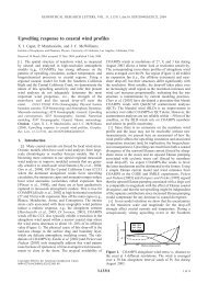
C05014 CHAIGNEAU AND PIZARRO: CIRCULATION OF THE EASTERN SOUTH PACIFIC
spatial decorrelation scales, and diffusivity, along with error
estimates. We also determine the respective contributions of
horizontal advection and turbulent diffusion on passive
tracer fluxes. Mean advective and eddy diffusive temperature
and salinity fluxes are thus estimated in the mixed layer
of the whole study region. The ensemble of the results
provides a useful tool for a comparison with the previous
studies but also for the validation of both regional and
global models in the eastern South Pacific.
[4] This work is organized as follows: section 2 describes
the data sets and processing methods used; section 3 deals
with the surface circulation and eddy kinetic energy; and
section 4 analyses Lagrangian scales of variability and eddy
diffusivity. In section 5, we estimate the respective role of
the large-scale advection and turbulent diffusive flow on the
mixed layer temperature and salinity fluxes. Finally, section
6 summarizes the study results.
2. Data Set
[5] The major data sets used in this study are surface
satellite-tracked drifters and Topex-Poseidon/ERS1-2 altimeters
measurements. Additionally, the World Ocean Atlas
2001 (WOA) climatology and satellite ERS winds are also
used. The study region extends from 10°S to34°Sand from
70°W to 100°W (Figure 1b).
[6] The surface satellite-tracked drifters data set spans
1979–2003 and is part of the Global Drifter Program/
Surface Velocity Program. The drifters were equipped with
a holey sock drogue centered at 15m depth in order to reduce
surface drag induced by both wind and waves. The expected
drogue slip relative to the water is less than 2 cm s 1 for
winds up to 20 m s 1 [Niiler and Paduan, 1995; Niiler et al.,
1995]. The Atlantic Oceanographic and Meteorological
Laboratory (AOML, Miami) received the drifter positions
from Doppler measurements from Service ARGOS. These
positions, irregularly distributed in time, were therefore
quality controlled and interpolated to uniform 6 hour intervals
using an optimum interpolation procedure [Hansen and
Poulain, 1996]. Velocity components were calculated by a
centered difference scheme at each 6 hour interval. In our
study area, a total of 476 different drifters, able to exit and
return to the area, were followed. To remove high-frequency
tidal and inertial wave energy and to avoid aliasing the
energy into the low-frequency motions, the four daily drifter
data were averaged over 24 hour intervals [Swenson and
Niiler, 1996; Martins et al., 2002]. A total of 72,244 daily
buoy position and velocity data were thus obtained from
1979 to 2003. Figure 1a shows the yearly distribution of the
number of daily observations. In the study region for all the
years between 1979 and 2003, the maximum amount of data
were observed during the 1990s, corresponding to the World
Ocean Circulation Experiment period, with a maximum of
9948 observations in 1993 and none in 1980 and 1984. The
results did not differ significantly when considering data
from the last decade (1991–2003) or the entire study period,
although the number of degrees of freedom was decreased.
In order to reduce the errors, we thus prefer use the whole
drifter data set. All seasons of the year were equally sampled
(not shown), with a minimum of around 15,000 observations
in austral summer (January to March) and a maximum of
20,000 in austral spring (October to December). The results
2of17
obtained hereafter are thus representative of an annual mean
state. Figure 1b shows the spatial coverage of the daily
data (shading) in the study region, and the number of
degrees of freedom or independent observations (see section
3.1 for calculation explanation). The bins have a minimum
size of 2° 2° latitude-longitude and are adjusted, especially
along the Chilean coast, to contain more than 6 independent
observations. Only 33 of the 152 cells contained less than 20
independent data. The southwestern part of the region was
extensively sampled, with more than 70 independent observations
in each bin south of 24°S and west of 84°W. In
contrast, along the continental coast, the grid cells contain
only between 6 and 35 degrees of freedom. For practical
reasons, we have chosen 50 daily data or 6 independent
observations as a lower limit, to make a compromise
between reasonable grid cell dimensions and robustness of
the results.
[7] The satellite altimetry data set used in this study is the
gridded product of Topex/Poseidon, ERS-1/2, and Jason-1
sea level anomalies (SLA) provided by Archiving Validation
and Interpretation of Satellite Data in Oceanography
(AVISO). This data set spans 1993–2003, with weekly SLA
distributed on a 1/3° Mercator Grid. The methods used to
process the data and reduce the errors are described by Le
Traon et al. [1995] and Le Traon and Ogor [1998] and by
Ducet et al. [2000]. Zonal and meridional components of
the residual sea surface velocity components were calculated
from the SLA, using the geostrophic relationship
V 0 g
U 0 g
¼ g
f
¼ g
f
@ ðSLAÞ @y
@ ðSLAÞ ;
@x
where g is the acceleration due to gravity, f is the Coriolis
parameter, and @x and @y are the eastward and northward
distances.
[8] Time mean eddy kinetic energy (per unit of mass),
EKE, is calculated using
EKE ¼ 1
2
U 0 2
g þ V 0 2
g
where the overbar denotes time average.
[9] Monthly temperature and salinity climatologies on a
1/4° latitude 1/4° longitude grid from the World Ocean
Atlas were used to estimate surface geostrophic velocities
relative to 1750 m depth. Generally, the common reference
level is chosen at around 3500 m in the study region
[Shaffer et al., 2004; Leth et al., 2004], but as this area
is one of the least-sampled of the world oceans, the use of
a climatology down to 3500 m may introduce important
errors rather than improve our results. Furthermore, based
on three hydrographic sections, Leth et al. [2004] show
that the maximum horizontal velocity between 1750 m and
3500 m depth is less than 0.02 cm s 1 in the study area.
Therefore we suppose that the 1750 m reference level does not
introduce a significant error in the surface velocity calculation.
In contrast to geostrophic velocities estimated from
;
C05014