Chaigneau and Pizarro - LEGOS

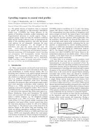
C05014 CHAIGNEAU AND PIZARRO: CIRCULATION OF THE EASTERN SOUTH PACIFIC
Figure 4. Spatial distribution of eddy kinetic energy from (a) drifter data and (b) satellite altimeter
measurements of TP/ERS. Bold lines show the SPC, SEC, and PCC.
the tracer evolution. In a Lagrangian frame, the most
common is that the velocity field can be decomposed in a
mean flow U =(U, V) representative of large spatial scale,
and in a turbulent mesoscale flow u 0 =(u 0 , v 0 ) computed
following the fluid particles [Poulain and Niiler, 1989;
Bauer et al., 1998, 2002; Kundu and Cohen, 2000]. Thus
the mean current U is determined by averaging the velocity
components over each drifter trajectory. The main properties
of the turbulent velocity field u 0 are the Lagrangian integral
time and length scales (T and L, respectively), which
represents the time and the distance over which a particle
remembers its path.
[26] For each component of the turbulent velocities (u 0 , v 0 ),
we can determine a temporal scale T =(T u, T v) by integrating
the respective velocity autocovariance function R =(R u, R v)
to its first zero crossing G [Taylor, 1921]:
T ¼ 1
Rð0Þ
Z G
0
RðtÞdt:
8of17
C05014
The Lagrangian autocovariance functions Ru (t) =
u0ðÞu t 0ðtþtÞ and Rv (t) =v0ðÞv t 0ðtþtÞ (here the overbar
denotes ensemble average) were determined for each drifter
spending more than 20 days in the domain and averaged in
time. A total of 353 drifter trajectories, assumed to be
independent, were then used to calculate this mean
autocovariance function. If a drifter exits the area and
returns several days later, the two different trajectories are
considered distinctly. Figure 5a shows the mean autocovariance
functions. The zonal and meridional components have
an e-folding scale (time lag at which the normalized
autocorrelation functions fall to 1/e = 0.368) of 4.1 days and
3.7 days, respectively; their first zero crossings are 50 and
16 days.
[27] Figure 5b shows the integral timescales of the
normalized autocovariance functions and indicates that the
zonal components converge between 50 and 90 days and
the meridional components between 15 and 25 days. After
these periods, the autocorrelation functions still statistically
converge to zero (Figure 5a), but as they are slightly