A Generic and Scalable Pipeline for GPU Tetrahedral Grid ... - TUM

A Generic and Scalable Pipeline
for GPU Tetrahedral Grid Rendering
Joachim Georgii ∗ Rüdiger Westermann †
Computer Graphics & Visualization Group, Technische Universität München
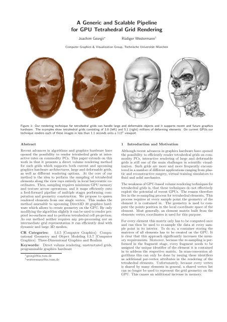
Figure 1: Our rendering technique for tetrahedral grids can handle large and deformable objects and it supports recent and future graphics
hardware. The examples show tetrahedral grids consisting of 3.8 (left) and 5.1 (right) millions of deforming elements. On current GPUs our
technique renders each of these images in less than 1.1 seconds onto a 512 2 viewport.
Abstract
Recent advances in algorithms and graphics hardware have
opened the possibility to render tetrahedral grids at interactive
rates on commodity PCs. This paper extends on this
work in that it presents a direct volume rendering method
for such grids which supports both current and upcoming
graphics hardware architectures, large and deformable grids,
as well as different rendering options. At the core of our
method is the idea to perform the sampling of tetrahedral
elements along the view rays entirely in local barycentric coordinates.
Then, sampling requires minimum GPU memory
and texture access operations, and it maps efficiently onto
a feed-forward pipeline of multiple stages performing computation
and geometry construction. We propose to spawn
rendered elements from one single vertex. This makes the
method amenable to upcoming Direct3D 10 graphics hardware
which allows to create geometry on the GPU. By only
modifying the algorithm slightly it can be used to render perpixel
iso-surfaces and to perform tetrahedral cell projection.
As our method neither requires any pre-processing nor an
intermediate grid representation it can efficiently deal with
dynamic and large 3D meshes.
CR Categories: I.3.5 [Computer Graphics]: Computational
Geometry and Object Modeling I.3.7 [Computer
Graphics]: Three-Dimensional Graphics and Realism
Keywords: Direct volume rendering, unstructured grids,
programmable graphics hardware
∗ georgii@in.tum.de
† westermann@in.tum.de
1 Introduction and Motivation
Although recent advances in graphics hardware have opened
the possibility to efficiently render tetrahedral grids on commodity
PCs, interactive rendering of large and deformable
grids is still one of the main challenges in scientific visualization.
Such grids are more and more frequently encountered
in a number of different applications ranging from plastic
and reconstructive surgery, virtual training simulators to
fluid and solid mechanics.
The weakness of GPU-based volume rendering techniques for
tetrahedral grids is, that these techniques do not effectively
exploit the potential of recent GPUs. The reason therefore
lies in the re-sampling process for tetrahedral elements. This
process requires at every sample point the geometry of the
element it is contained in. The geometry is used to compute
the points position in the local coordinate space of the
element. Most generally, an element matrix built from the
elements vertex coordinates is used for this purpose.
For every element this matrix only has to be computed once
and can then be used to re-sample the data at every sample
point in its interior. To do so, a container storing the
matrices of all elements has to be created on the GPU. It
is clear that this approach significantly increases the memory
requirements. Moreover, because the re-sampling is performed
in the fragment stage, every fragment needs to be
assigned the unique identifier of the element it is contained
in to address the respective matrix. In scan-conversion algorithms
this can only be done by issuing these identifiers
as additional per-vertex attributes in the rendering of the
tetrahedral elements. Unfortunately, because every vertex
is shared by many elements in general, a shared vertex list
can no longer be used to represent the grid geometry on the
GPU. This causes an additional increase in memory.

To avoid the memory overhead induced by precomputations,
element matrices can be calculated in
turn for every sample point. But then the same computations,
including multiple memory access operations to
fetch the respective coordinates, have to be performed
for all sample points in the interior of a single element,
thereby wasting a significant portion of the GPUs compute
power. As before, identifiers are required to access vertex
coordinates, and thus a shared vertex array cannot be used.
1.1 Contribution
In this paper we present a GPU pipeline for the rendering of
tetrahedral grids that avoids the aforementioned drawbacks.
This pipeline is scalable with respect to both large data sets
as well as future graphics hardware. The proposed method
has the following properties:
• Per-element calculations are performed only once.
• Tetrahedral vertices and attributes can be shared in
vertex and attribute arrays.
• Besides the shared vertex and attribute arrays no additional
memory is required on the GPU.
• Re-sampling of (deforming) tetrahedral elements is performed
using a minimal memory footprint.
1.2 System Overview
To achieve our goal we propose a generic and scalable GPU
rendering pipeline for tetrahedral elements. This pipeline is
illustrated in Figure 2. It consists of multiple stages performing
element assembly, primitive construction, rasterization
and per-fragment operations.
Figure 2: Overview of the GPU rendering pipeline.
To render a tetrahedral element the pipeline is fed with one
single vertex, which carries all information necessary to assemble
the element geometry on the GPU. This stage is described
in Section 3.1. Assembled geometry is then passed
to the construction stage where a renderable representation
is built.
The construction stage is explicitly designed to account for
the functionality on upcoming graphics hardware. With Direct3D
10 compliant hardware and geometry shaders [1] it
will be possible to create additional geometry on the graphics
subsystem. In particular, triangle strips or fans composed
of several vertices, each of which can be assigned individual
per-vertex attributes, can be spawned from one single
vertex. As the geometry shader itself can perform arithmetic
and texture access operations, these attributes can be
computed in account of the application specific needs. By
using the aforementioned functionality the renderable representation
can be constructed in turn without sacrificing
the feed-forward nature of the proposed rendering pipeline.
Section 3.2 gives in-depth details on this stage.
As hardware-assisted geometry shaders are not yet available
on current GPUs we have implemented the proposed
pipeline using the DirectX9 SDK. This SDK provides a software
emulation of the entire Direct3D 10 pipeline, and it is
available under the recent Microsoft Vista beta version. Unfortunately,
neither does this emulation provide meaningful
performance measures nor does it allow to estimate relative
timings between the pipeline stages. Nevertheless, the implementation
using this software emulation clearly demonstrates
that the proposed pipeline concept can effectively be
mapped onto upcoming GPUs in the very near future.
To verify the efficiency of the intended method we propose
an emulation of the primitive construction step using the
render-to-vertexbuffer functionality. The specific implementation
will be discussed in Section 6. Although this emulation
requires additional rendering passes it still results in
frame rates superior to those that can be achieved by the
fastest methods known so far.
The renderable representation is then sent to the GPU rasterizer.
On the fragment level a number of different rendering
techniques can be performed for each tetrahedron,
including a ray-based approach, iso-surface rendering and
cell projection. The discussion in the remainder of this paper
will be focused on the first approach, and we will briefly
describe the other rendering variants in Sections 4 and 5.
The ray-based approach operates similar to ray-casting by
sampling the data along the view rays. In contrast, however,
it does not compute for each ray the set of elements consecutively
hit along that ray, but it lets the rasterizer compute
for each element the set of rays intersecting that element.
The interpolation of the scalar field at the sample points in
the interior of each element is then performed in the fragment
stage, and the results are finally blended into the color
buffer.
The approach as described requires the tetrahedral elements
to be sampled in correct visibility order. To avoid the explicit
computation of this ordering we first partition the eye
coordinate space into spherical shells around the point of
view. Figure 3 illustrates this partitioning strategy.
Figure 3: Ray-based tetrahedra sampling.
These shells are consecutively processed in front-to-back order,
simultaneously keeping the list of elements overlapping
the current shell. Intra-shell visibility ordering is then
achieved by re-sampling the elements onto spherical slices
positioned at equidistant intervals in each shell (see right
of Figure 3). In Section 3.3 we will show how to efficiently
perform the re-sampling using multiple render targets.
To minimize the number of arithmetic and memory access
operations the re-sampling procedure is entirely performed
in barycentric coordinate space of each element. This ap-

proach has some important properties: First, barycentric
coordinates of sample points can directly be used to interpolate
the scalar values given at grid vertices. Second,
barycentric coordinates can efficiently be used to determine
whether a point lies inside or outside an element. Third, by
transforming both the point of view and the view rays into
the barycentric coordinate space of an element, barycentric
coordinates of sample points along the rays can be computed
with a minimum number of arithmetic operations. Fourth,
barycentric coordinates of vertices as well as barycentric coordinates
of the view rays through the vertices can be issued
as per-vertex attributes, which then get interpolated across
the element faces during rasterization.
1.3 Related Work
Object-space rendering techniques for tetrahedral grids accomplish
the rendering by projecting each element onto the
view plane to approximate the visual stimulus of viewing the
element. Two principal methods have been shown to be very
effective in performing this task: slicing and cell projection.
Slicing approaches can be distinguished in the way the computation
of the sectional polygons is performed. This can
either be done explicitly on the CPU [29, 33], or implicitly
on a per-pixel basis by taking advantage of dedicated
graphics hardware providing efficient vertex and fragment
computations [22, 26, 28].
Tetrahedral cell projection [17], on the other hand, relies
on explicitly computing the projection of each element onto
the view plane. Different extensions to the cell-projection
algorithm have been proposed in order to achieve better accuracy
[21, 31] and to enable post-shading using arbitrary
transfer functions [16]. GPU-based approaches for cell projection
have been suggested, too [23, 25, 32].
The most difficult problem in tetrahedral cell projection is
to determine the correct visibility order of elements. The
most efficient way is PowerSort [3, 8], which exploits the
fact that for tetrahedral meshes exhibiting a Delaunay property
the correct order can be found by sorting the tangential
distances to circumscribing spheres using any customized algorithm.
As grids in practical applications are usually not
Delaunay meshes this approach might lead to incorrect results
and does not allow resolving topological cycles in the
data.
A different alternative is the sweep-plane approach [7, 18, 19,
27]. In this approach the coherence within cutting planes in
object space is exploited in order to determine the visibility
ordering of the available primitives. In addition, much
work has been spent on accelerating the visibility ordering
of unstructured elements. The MPVO method [30], and
later extended variants of it [4, 20], were designed to take
into account topological information for visibility ordering.
Techniques using convexification to make concave meshes
amenable to MPVO sorting have been proposed in [15]. Recently
a method to overcome the topological sorting of unstructured
grids has been presented [2]. By using an initial
sorter on the CPU a small set of GPU-buffers can be used
to determine the visibility order on a per-fragment basis.
Based on the early work on GPU ray-casting [13] a raybased
approach for the rendering of tetrahedral grids has
been proposed in [24].
Besides the direct volume rendering of tetrahedral grids
there has also been an ongoing effort to employ GPUs for
iso-surface extraction in such grids [5]. The calculation of
the iso-surface inside the tetrahedral elements was carried
out in the vertex units of programmable graphics hardware
[12, 14]. Significant accelerations were later achieved by employing
parallel computations and memory access operations
in the fragment units of recent GPUs in combination with
new functionality to render constructed geometry without
any read-back to the CPU [9, 10].
2 Data Representation and Transfer
The tetrahedral grid is maintained in the most compact representation:
a shared vertex array that contains all vertex coordinates
and an index array consisting of one 4-component
entry per element. Each component represents an index into
the vertex array. While the index array only resides in CPU
memory, the vertex array is stored on the CPU, and as a 2D
floating point texture on the GPU. Additional per-vertex
attributes like scalar or color values are only hold on the
GPU.
By assigning to each vertex a 3D texture coordinate it is also
possible to bind a 3D texture map to the tetrahedral grid.
By one additional texture indirection the scalar or color values
can then be sampled via interpolated texture coordinates
from a 3D texture map. This strategy is in particular useful
for the efficient rendering of deforming Cartesian grids.
By deforming the geometry of a tetrahedral grid but keeping
the 3D texture coordinates fix, the deformed object can
be rendered at much higher resolution compared to just linear
interpolation of the scalar field given at the displaced
tetrahedra vertices.
To render a tetrahedral grid the CPU computes for each
spherical shell the set of elements (active elements) overlapping
this shell. Each time a shell is to be rendered the
CPU uploads this active element list, represented as a 4component
index array. This list is then passed through the
proposed rendering pipeline.
3 Tetrahedral Grid Rendering
In this section we describe the rendering pipeline for tetrahedral
grids, which is essentially a sampling of the attribute
field at discrete points along the view rays through the grid.
The sampling process effectively comes down to determining
for each sampling point the tetrahedron that contains
this point as well as the points position in local barycentric
coordinates of this tetrahedron. Due to this observation we
decided to rigorously perform the rendering of each element
in local barycentric space, thus minimizing the number of
required element and fragment operations. Figure 4 shows
a conceptual overview of the entire rendering pipeline for
tetrahedral grids. For the sake of clarity, pseudo-code notation
is given in Appendix A.
3.1 Element Assembly
For every shell to be rendered the active element list contains
one vertex per element, each of which stores four references
into the vertex texture. In the element assembly stage these

Figure 4: Data stream overview
indices are resolved by interpreting them as texture coordinates.
Via four texture access operations the four vertices
are obtained, and they are then transformed into eye coordinate
space. Both the four indices as well as the transformed
vertices are passed to the primitive construction stage.
3.2 Primitive Construction
The primitive construction stage generates all the information
that is used in the upcoming stages but only needs to be
computed once per element. First, for every element the matrix
required to transform eye coordinates into local barycentric
coordinates is computed. The vertices, given in homogeneous
eye coordinates, are denoted by vi, i ∈ {0, 1, 2,3}.
The transformation matrix can then be computed as
B = � v0 v1 v2 v3
� −1 .
Next, for every element the eye position veye = (0,0, 0,1) T
is transformed into its barycentric coordinate space: beye =
B veye. It is important to note that only the last column
of B is required thus significantly reducing the number of
arithmetic operations to be performed. The barycentric coordinates
of each of the vertices vi are given by the canonical
unit vectors ei. Finally, the directions of all four view rays
passing through the element vertices are transformed into
barycentric coordinates via bi = ei − beye. As the mapping
from eye coordinate space to barycentric coordinate space is
affine, these directions can later be interpolated across the
element faces. In addition, the length of the view vector,
li = ||vi − veye||2, is computed for every vertex in the primitive
construction stage. It is used in the fragment stage to
normalize the barycentric ray directions bi.
Once the aforementioned per-element computations have
been performed, each tetrahedron is rendered as a triangle
strip consisting of four triangles. These strips are composed
of the six element vertices, which are first transformed to
normalized device coordinates. To each of these vertices
the respective bi, the barycentric eye position beye and the
length of the view vector li are assigned as additional pervertex
attributes, i.e. texture coordinates. Moreover, four
per-element indices into the GPU attribute array are assigned
to each vertex. These indices are later used in the
fragment stage to access the scalar field or the 3D texture
coordinates used to bind a texture map.
The rasterizer generates one fragment for every view ray
passing through a tetrahedron, and it interpolates the given
per-vertex attributes. To reduce the number of generated
fragments only front-faces are rendered using API built-in
culling functionality.
3.3 Fragment Stage
When rendering the primitives composed of attributed vertices
as described, the rasterizer interpolates the bi and li
and generates for every fragment a local barycentric ray direction
b as well as its length l in eye coordinates. By using
the barycentric coordinates of the eye position beye, the view
ray in local barycentric space can be computed for every
fragment as (t denotes the ray parameter)
b
· t + beye, t > 0.
l
This ray is sampled on a spherical slice with distance zs from
the eye point. The barycentric coordinate of the sample
point is obtained by setting t as the depth of the actual
spherical slice, zs.
It is now clear that a fragment has all the information to
determine the barycentric coordinates of multiple sample
points along the ray passing through it. If an equidistant
sampling step size ∆zs along the view rays is assumed, the
coordinates of every point are determined as
b k = b
· (zs + k · ∆zs) + beye, k ∈ {0, 1, . . . , n − 1}. (1)
l
where n is the number of samples. The fragment program
obtains the depth zs of the first sample point and the sample
spacing ∆zs as constant parameters.
A fragment can trivially decide whether a sample point is inside
or outside the tetrahedron by comparing the minimum
of all components of b k with zero. A minimum greater or
equal to zero indicates an interior point. In this case the
sample point is valid and thus has a contribution to the accumulated
color along the ray. Otherwise, the sample point
is invalid and has to be discarded.
The barycentric coordinates are directly used to interpolate
per-vertex attributes. This can be scalar values that are
first looked up from the attribute texture via the issued pervertex
indices, or it can be a 3D texture coordinate that is
then used to fetch a scalar value from a texture map. Finally,
each fragment has determined one scalar value for each of
its n samples.
Once the scalar field has been re-sampled onto a number of
sample points along the view-rays these values can in principle
be directly composited in the fragment program. Unfortunately,
as the elements within one spherical cell have
not been rendered in correct visibility order this would lead
to visible artifacts. On the other hand we can write four
scalar values at once into a RGBA render target. Moreover,
recent graphics APIs allow for the simultaneous rendering
into multiple render targets. This means that up to four
times the number of render targets spherical slices can be
re-sampled by one single fragment. Sampled values are rendered
into the respective component and render target using
a max blend function. If a sample point is outside the element,
a zero value is written into the texture component
and the sample is ignored. As no two tetrahedra can contain
the same sample point along either ray, erroneous results are
avoided.
The number of samples that can be processed efficiently at
once is restricted by the output bandwidth of the fragment
program. Because up to 128 bits can be rendered simultaneously
on recent GPUs, up to 16 slices can be processed

at once if 8 bit scalar values are assumed. This implies that
every spherical shell is as thick as to contain exactly 16 slices
with regard to the current sampling step size. In account of
this number, four additional texture render targets have to
be used to keep intermediate sampling results. Without utilizing
the multiple render target extension, still four samples
can be processed at once.
3.4 Blending Stage
In the final stage up to four texture render targets are
blended into the frame buffer. In each of its four components
these textures contain the sampled scalar values on
one spherical slice of the shell. The blending stage now performs
the following two steps in front-to-back order. First,
scalar values are mapped to color values via a user-defined
transfer function. Second, a simple fragment program performs
the blending of the color values via alpha-compositing
and finally outputs the results to the frame buffer.
4 Iso-Surface Rendering
To avoid explicit construction of geometry on the GPU, perpixel
iso-surface rendering can be integrated into our proposed
rendering pipeline easily. Instead of sampling all the
values along the view-rays only the intersection points between
these rays and the iso-surface are determined on a
per-fragment basis. Thereby, the primitive assembly and element
construction stage remain unchanged, and only the
fragment stage needs minor modifications.
Given an iso-value siso, the view-ray passing through a fragment
intersects the iso-surface at depth
tiso = siso − �4 si · (beye)i
i=0
�4 si · (b)i
i=0
This formula is derived from the condition that the scalar
value along the ray (given in local barycentric coordinates)
should equal the iso-value. It is worth noting that tiso is
undefined if the denominator is zero. In this case the interpolated
scalar values along the ray are constant, and we
can either choose any valid value for tiso if the scalar value
is equal to siso or the ray has no intersection with the isosurface.
The computed barycentric coordinate b · tiso + beye of the
intersection point is tested against the tetrahedron as described
above. Only if the point is in the interior of the
element an output fragment is generated. Otherwise the
fragment is discarded.
In this particular rendering mode the data representation
stage has to be modified slightly. Instead of building an
active element list for every shell, only one list that contains
all elements being intersected by the iso-surface is built.
These tetrahedra can then be rendered in one single pass, or
in multiple passes if more elements are intersected by the
surface than can be stored in a single texture map. The
blending stage becomes obsolete and can be replaced by the
standard depth test to keep the front-most fragments in the
frame buffer. A fragments’ depth value is set to the depth
of the intersection point in the fragment program. Finally,
it should have become clear from the above description that
per-element gradients can be computed in the primitive construction
stage as well. Gradients are assigned as additional
per-vertex attributes to the fragment stage for lighting calculations.
5 Cell Projection
Tetrahedral cell projection is among the fastest rendering
techniques for unstructured grids as every element is only
rendered ones. However, it requires a correct visibility ordering
of the elements, and it can be time consuming to achieve
such an ordering in general. To demonstrate tetrahedral cell
projection we employ the tangential distance or power sort
[8] on the CPU to determine an approximate ordering.
Tetrahedral cell projection can be achieved by a slight modification
of the fragment stage. Given the fragments’ depth
zin, the barycentric coordinates of this fragment can be computed
as
bin = b/l · zin + beye. (2)
The intersection with each of the faces of the corresponding
tetrahedron can be calculated by using the ray equation
bout = b/l · t + beye in barycentric coordinates. To compute
bout, four candidate parameters tl, l ∈ {0, 1,2, 3} are obtained
by alternately setting the components of bout to zero.
As the ray parameter t = zin corresponds to the entry point
of the ray, the value of t at the exit points is determined by
zexit = min{tl : tl > zin}.
The barycentric coordinate of the exit point can then be
derived according to equation (2).
From the barycentric coordinates of the entry and exit point
the length of the ray segment being inside the tetrahedron
can be calculated. This information is required to compute
a correct attenuation value for every fragment [17]. The
barycentric coordinates are used to obtain scalar values at
the entry and exit point, which are then integrated along the
ray.
6 Implementation
As current graphics hardware does not support geometry
shaders to construct geometry on the GPU, the primitive
assembly stage and the primitive construction stage are simulated
via multiple rendering passes.
Once the CPU has uploaded the index texture to the GPU
(see Section 2), a quad covering four times as many fragments
as active elements is rendered. Every fragment reads
the respective index and performs one dependent texture
fetch to get the corresponding vertex coordinate. The 4th
component of each vertex is used to store the element index.
This index is used in the final fragment stage to fetch the
barycentric transformation matrix. The vertex coordinates
are written to a texture render target, which is either copied
into a vertex array (on NVIDIA cards) or directly used as a
vertex array (on ATI cards). In this pass, the transformation
of vertices into eye coordinates can already be performed.
In a second pass, each active tetrahedron reads its four vertices
as described and computes the last row of the barycentric
transformation matrix, beye, which is stored in a RGBA

float texture. Due to the fact that only one index per tetrahedron
can be stored, we also built a RGBA texture that
stores for every active element the four attached scalar values
in one single texel. If 3D texture coordinates are required
they are stored analogously in three RGBA textures.
We then use an additional index array to render the tetrahedral
faces. We either use 7 indices per tetrahedron to
render a triangle strip followed by a primitive restart mark
(on NVIDIA cards only) or we use 12 indices to render the
tetrahedral faces separately. Note that the index array does
not change and can be kept in local GPU memory.
Finally, the fragment stage has to be modified such that every
fragment now fetches beye and performs all operations
required to sample the element along the view-rays in local
barycentric space. Although this increases the number
of arithmetic and memory access operations considerably,
we will show later that the implementation already achieves
impressive frame rates on recent graphics hardware.
7 Results
In the following we present some results of our algorithm,
and we give timings for different parts of it. All test were run
on a single processor Pentium 4 equipped with an NVIDIA
7900 GTX graphics processor. The size of the viewport was
set to 512 × 512.
We have tested the tetrahedral rendering pipeline for both
static and deformable meshes. For the simulation of physicsbased
deformations we have employed the Multigrid framework
proposed in [6]. The GPU render engine receives computed
displacements and updates the geometry of a volumetric
body accordingly. While the simulation engine consecutively
displaces the underlying finite element grid, the render
engine subsequently changes the geometry of the volumetric
render object. It is worth noting, on the other hand, that all
timings presented in this paper exclude the amount of time
required by the simulation engine. In all our examples the
time required to send updated vertices to the GPU is below
3% of the overall rendering time.
The proposed technique for direct volume rendering of unstructured
grids is demonstrated in Figures 5 to 7. Table
1 shows performance rates on our target architecture implementing
the rendering pipeline described in Section 6.
Timing statistics for alternative rendering modes are given
in Table 2. Volume rendered imagery using cell projection
and iso-surface rendering is shown in Figures 8 and 9.
The first four rows of Table 1 show the number of tetrahedral
mesh elements, the number of sample points per ray,
the number of samples per shell and the total number of
elements being rendered. As elements are likely to overlap
more than one shell, this number is approximately 2 times
higher than the mesh element count. Next, GPU memory
requirements (excluding 3D texture maps) are shown. The
memory required by the vertex, scalar and blend textures
is listed. Additional memory that is due to the emulation
of the construction stage on current GPUs is summarized in
the next row.
As can be seen, the proposed rendering pipeline exploits the
limited GPU memory very effectively. On the other hand,
even if the mesh does not fit into local GPU memory the
method can still be used very efficiently. One possibility
is to partition the grid, and thus the vertex and attribute
textures, into equally sized blocks. These blocks can then be
rendered in multiple passes, which only requires a separate
active element list for each partition and shell.
The upcoming rows in Table 1 give detailed timings of the
different rendering modes. All timings are given in milliseconds.
Starting with the time required by the CPU to calculate
the active element sets and to transfer all required
data to the GPU, timings for GPU primitive assembly and
construction as well as per-fragment computations are given.
scene horse bluntfin engine vmhead
# Tetrahedra 50k 190k 1600k 3800k
# Samples / ray 300 400 500 600
# Samples / shell 4 8 8 8
# Tets rendered 133k 434k 3438k 6618k
vertices/scalars [MB] 0.27 1.1 17 17
blend textures [MB] 1 2 2 2
intermediate [MB] 3.3 13 13 13
GPU memory [MB] 4.6 16.1 32 32
CPU [ms] 4 12 101 244
GPU Geometry [ms] 11 12 65 135
GPU Fragments [ms] 43 85 445 732
Total time [ms] 58 109 611 1111
Table 1: Element, memory and timing statistics for various data sets.
scene horse bluntfin engine vmhead
Iso-Value 0.5 0.2 0.5 0.27
Iso-Surface [ms] 4.6 5.7 51 124
Cell Projection [ms] 19 54 341 1176
Table 2: Timing statistics for different rendering modes.
From the timing statistics the following can be perceived:
Although the current implementation introduces a significant
overhead in terms of arithmetic and memory access operations
and requires additional memory on the GPU, performance
rates similar to the fastest techniques so far can be
achieved. A maximum throughput of 1.8M tetrahedra/sec
has been reported recently by Cahallan et. al. [2] on an ATI
Radeon 9800. In comparison our pipeline already achieves a
peak rate that is over a factor of three higher. In particular
it can be seen that one of the drawbacks of slice-based techniques,
i.e. multiple rendering of elements, can significantly
be reduced due to the simultaneous evaluation of multiple
sample points. It is clear, however, that in case of elements
Figure 5: Close-up view of the bluntfin data set.

Figure 6: Direct volume rendering of the deformable visible human
data set. The tetrahedral mesh consists of 3.6 million elements, and
it is textured with a 512 2 × 302 3D texture map.
Figure 7: These images show direct volume rendering of a tetrahedral
mesh consisting of 1600k elements. A 3D texture of size 256 2 × 110
storing the engine data set is bound to the mesh.
Figure 8: Our method can efficiently be applied to visualize internal
states of deforming volumetric bodies. In the example, the internal
stress of the model under gravity is visualized in red using the cell
projection method.
that overlap only a very few slices some of these evaluations
might be wasted. For this reason we have chosen data dependent
numbers of slices as shown in Table 1.
The examples given in Figures 6 and 7 show the visualization
of deformable tetrahedral grids to which a 3D texture
map is bound. Every vertex stores coordinates into a 3D
texture map, which are interpolated in the fragment stage.
Interpolated coordinates are finally used to fetch the data
from the texture map.
Figure 9: Iso-surface rendering of the deformed visible male data set.
The tetrahedral mesh was adaptively refined to recover the skin and
bone structures, and it consists of 5.1 million elements. Per-vertex
scalar values were re-sampled from the original 3D data set. To
smooth-shade the iso-surface, per-vertex gradients are first accumulated
in every frame on the GPU, and they are finally interpolated in
the fragment stage via barycentric coordinates.
8 Conclusion
In this paper we have described a generic and scalable rendering
pipeline for tetrahedral grids. The pipeline is designed
to facilitate its use on recent and upcoming graphics
hardware and to accommodate the rendering of large and
deformable grids. In particular we have shown, that our concept
supports upcoming features on programmable graphics
hardware and thus has the potential to achieve significant
performance gains in the very near future.
The rendering pipeline we propose is ray-based in that it performs
the sampling of tetrahedral elements along the view
rays. It maps on a feed-forward pipeline that is spawned
by one single vertex. Per-element calculations have to be
performed only once, and the rasterizer is efficiently utilized
to minimize per-fragment operations. As the sampling is
entirely performed in local barycentric coordinates of each
element it requires minimum arithmetic and texture access
operations on the GPU. By enabling the evaluation of multiple
samples per element, we can significantly reduce the
number of rendered elements, because the number of elements
that overlap more than one shell decreases. As no
pre-processing of the grid data is required, it is perfectly
suited for the rendering of deformable meshes. Additional
rendering modes like iso-surface rendering and cell projection
can be integrated into this pipeline in a straight forward
way.
Besides the verification of our current results on future Direct3D
10 graphics hardware we will investigate the integration
of acceleration techniques for volume ray-casting into
the current approach. In particular, early-ray-termination
as proposed for texture-based volume ray-casting [11] seems
to be a promising acceleration strategy that perfectly fits
into our dedicated rendering pipeline.

References
[1] R. Balaz and S. Glassenberg. DirectX and Windows
Vista Presentations. http://msdn.microsoft.com/directx/archives/pdc2005/,
2005.
[2] S. Callahan, M. Ikits, J. Comba, and C. Silva. Hardwareassisted
visibility sorting for unstructured volume rendering.
In IEEE Transactions on Visualization and Computer
Graphics Vol. 11, 2005.
[3] P. Cignoni, C. Montani, D. Sarti, and R. Scopigno. On the
optimization of projective volume rendering. In EG Workshop,
Scientific Visualization in Scientific Computing, 1995.
[4] J. Comba, J. Klosowsky, N. Max, J. Mitchell, C. Silva, and
P. Willians. Fast polyhedral cell sorting for interactive rendering
of unstructured grids. In Proc. of Eurographics, 1999.
[5] A. Doi and A. Koide. An efficient method of triangulating
equi-valued surfaces by using tetrahedral cells. In IEICE
Transactions Commun. Elec. Inf. Syst., 1991.
[6] J. Georgii and R. Westermann. A multigrid framework for
real-time simulation of deformable volumes. In Workshop On
Virtual Reality Interaction and Physical Simulation, 2005.
[7] C. Giertsen. Volume visualization of sparse irregular meshes.
IEEE Comput. Graph. Appl., 1992.
[8] M. Karasick, D. Lieber, L. Nackman, and V. Rajan. Visualization
of three-dimensional delaunay meshes. In Algorithmica,
2003.
[9] P. Kipfer and R. Westermann. GPU construction and transparent
rendering of iso-surfaces. In Proceedings Vision, Modeling
and Visualization ’05, 2005.
[10] T. Klein, S. Stegmaier, and T. Ertl. Hardware-accelerated
Reconstruction of Polygonal Isosurface Representations on
Unstructured Grids. In Proceedings of Pacific Graphics ’04,
pages 186–195, 2004.
[11] J. Krüger and R. Westermann. Acceleration techniques for
GPU-based volume rendering. In IEEE Visualization, 2003.
[12] V. Pascucci. Isosurface computation made simple: Hardware
acceleration, adaptive refinement and tetrahedral stripping.
In Proc. of IEEE TCVG Symp. on Visualization, 2004.
[13] T. Purcell, I. Buck, W. Mark, and P. Hanrahan. Ray tracing
on programmable graphics hardware. ACM Computer
Graphics (Proc. SIGGRAPH ’02), 2002.
[14] F. Reck, C. Dachsbacher, R. Grosso, G. Greiner, and
M. Stamminger. Realtime isosurface extraction with graphics
hardware. In Eurographics Short Presentations, 2004.
[15] S. Röttger and T. Ertl. Cell projection of convex polyhedra.
In Proceedings Eurographics/IEEE TVCG Workshop
Volume Graphics ’03, 2003.
[16] S. Röttger, M. Kraus, and T. Ertl. Hardware-accelerated
volume and isosurface rendering based on cell-projection. In
Proceedings of IEEE Visualization ’00, pages 109–116, 2000.
[17] P. Shirley and A. Tuchman. A Polygonal Approximation to
Direct Scalar Volume Rendering. ACM Computer Graphics,
Proc. SIGGRAPH ’90, 24(5):63–70, 1990.
[18] C. Silva and J. Mitchell. The Lazy Sweep Ray Casting Algorithm
for Rendering Irregular Grids. Transactions on Visualization
and Computer Graphics, 4(2), June 1997.
[19] C. Silva, J. Mitchell, and A. Kaufman. Fast Rendering of
Irregular Grids. In Symp. on Volume Visualization, 1996.
[20] C. Silva, J. Mitchell, and P. Williams. An exact interactive
time visibility ordering algorithm for polyhedral cell complexes.
In VVS ’98: Proceedings of the 1998 IEEE symposium
on Volume visualization, 1998.
[21] C. Stein, B. Becker, and N. Max. Sorting and hardware
assisted rendering for volume visualization. In ACM Symposium
on Volume Visualization ’94, pages 83–90, 1994.
[22] M. Weiler and T. Ertl. Hardware-Software-Balanced Resampling
for the Interactive Visualization of Unstructured Grids.
In Proceedings of IEEE Visualization ’01, 2001.
[23] M. Weiler, M. Kraus, and T. Ertl. Hardware-based viewindependent
cell projection. In VolVis, 2002.
[24] M. Weiler, M. Kraus, M. Merz, and T. Ertl. Hardware-Based
Ray Casting for Tetrahedral Meshes. In Procceedings IEEE
Visualization, 2003.
[25] M. Weiler, M. Kraus, M. Merz, and T. Ertl. Hardware-Based
View-Independent Cell Projection. IEEE Transactions on
Visualization and Computer Graphics, 9(2), 2003.
[26] R. Westermann. The rendering of unstructured grids revisited.
In EG/IEEE TCVG Symposium on Visualization
(VisSym ’01), 2001.
[27] R. Westermann and T. Ertl. The VSBUFFER: Visibility Ordering
unstructured Volume Primitives by Polygon Drawing.
In IEEE Visualization ’97, pages 35–43, 1997.
[28] R. Westermann and T. Ertl. Efficiently using graphics hardware
in volume rendering applications. In ACM SIGGRAPH
1998, 1998.
[29] J. Wilhelms, A. Van Gelder, P. Tarantino, and J. Gibbs. Hierarchical
and parallelizable direct volume rendering for irregular
and multiple grids. In IEEE Visualization ’96, 1996.
[30] P. Williams. Visibility Ordering Meshed Polyhedra. ACM
Transactions on Graphics, 11(2):102–126, 1992.
[31] P. Williams, N. Max, and C. Stein. A high accuracy volume
renderer for unstructured data. IEEE Transactions on
Visualization and Computer Graphics, 4(1), 1998.
[32] B. Wylie, K. Moreland, L. Fisk, and P. Crossno. Tetrahedral
projection using vertex shaders. In VVS ’02: Proceedings
of the 2002 IEEE symposium on Volume visualization and
graphics, 2002.
[33] R. Yagel, D. Reed, A. Law, P. Shih, and N. Shareef. Hardware
assisted volume rendering of unstructured grids by incremental
slicing. In VVS ’96: Proceedings of the 1996 symposium
on Volume visualization, 1996.
A Pseudo-code snippets for ray-based GPU tetrahedron
rendering
elementAssembly (index)
for i = 0, . . . , 3
vi = texture(vertexTex, indexi);
vi = Modelview ∗ vi;
return (index, v0, v1, v2, v3);
primitiveConstruction (index, v0, v1, v2, v3)
B = inverse ((v0, v1, v2, v3));
beye = B ∗ (0, 0, 0, 1) T ;
for i = 0, . . . , 3
li = length(vi − (0, 0, 0, 1) T );
bi = ei − beye;
vi = Projection ∗ vi;
Rasterize strip
� � � � � � � � � � � �
v0 v1 v2 v3 v0 v1
b0
,
b1
l0 l1 l2
return (index, beye);
,
b2
fragmentStage(interpol. v, interpol. b, interpol. l,
index, beye, const zs, const ∆zs)
for i = 0, . . . , 3
s[i] = texture(scalarsTex, indexi);
for k = 0, . . . , n
bc = beye + b/l ∗ (zs + k ∗ ∆zs);
if min(bc[0], bc[1], bc[2], bc[3]) < 0
out[k] = 0;
else
out[k] = dot(s, bc);
return (out);
,
b3
l3
,
b0
l0
,
b1
l1