Statistical properties of determinantal point processes in high ...

SCARDICCHIO, ZACHARY, AND TORQUATO PHYSICAL REVIEW E 79, 041108 2009
Other ensembles of two-dimensional determinantal point
processes can be found in simple systems. For example, the
n zeros of an analytic Gaussian random function fz
n
=k=0akzk also form a determinantal point process on the
open unit disk 28,29. The limiting kernel governing these
zeros is called the Bargmann kernel:
Hz1,z 2 = 1 1
1−z1z22 63
and is inherently different from 59.
IV. AN ALGORITHM FOR GENERATING
DETERMINANTAL POINT PROCESSES
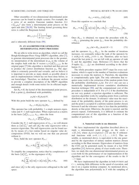
We are able to write down an algorithm, which we call the
Hough-Krishnapur-Peres-Virag HKPV algorithm, after 7,
to generate determinantal point processes due to the geometric
interpretation of the determinant in N as the volume of
the simplex built with the N vectors v j= j
0 1jN. Inthe
original paper 7 this algorithm is sketched and then proved
to produce the correct distribution function p N. The algorithm
is extremely powerful and versatile, and we believe it
is important to provide as many details as possible about it
and its implementation which has not been done before, to
our knowledge. Therefore, we dedicate the present section
to provide a complete description of the HKPV algorithm
and enough details with some tricks for its efficient implementation.
Set H NH, the kernel of the determinantal point process.
Pick a point N distributed with probability
pNx = HNx,x/N. 64
With this point build the new operator AN−1, defined by
A N−1 = H N N NH N. 65
This operator has with probability 1 a single nonzero eigen-
value and N−1 null eigenvalues. When expressed as a matrix
0
in the basis n1nN, AN−1 takes the form
0 0
AN−1i,j = i N j N. 66
Consider the N−1 null eigenvectors of AN−1; we will denote
1 N−1 1
them as i i=1 and call N
the only eigenvector with a
nonzero eigenvalue. The null eigenvectors can be found easily
by means of a fast routine based on singular value decomposition
SVD, but we will see one that can proceed
without it.
Next, build the new operator HN−1: N−1
1 1
HN−1 = HN nnHN. 67
n=1
To simplify the computation, notice that by completeness of
1 N
the basis nn=1 in the eigenspace of HN: N−1
H N n=1
1 1 1 1
nn + NNHN
= HN, 68
1
and since N is the only eigenvector orthogonal to the null
space:
041108-8
1 1
AN−1 =trAN−1NN. 69
From this equation we conclude that
N−1
H N−1 H N n=1
1 1 1
nnHN = HNI −
trAN−1 AN−1HN. 70
Once H N−1 is obtained, we repeat the procedure with H N
→H N−1, generating the point N−1 from the probability distribution
p N−1x = H N−1x,x/N −1 71
and the operators A N−2, H N−2. As the number of iterations
increases, we constantly reduce the rank of the operators by
1: trH N=N, trH N−1=N−1, etc. Therefore, after we have
placed the last point 1, we are left with an operator of rank
0, and the algorithm stops. Reference 7 shows that the
N-tuples 1,..., N are distributed according to the distribution
1.
The whole procedure requires ON 2 steps for every realization,
which is equal to the number of function evaluations
necessary to create the matrices A. Therefore, the algorithm
is computationally quite light. The only subroutine that requires
some work is the extraction of the random points from
the probability distributions p nx. For d=1 one can use a
numerically implemented inverse cumulative distribution
function technique 30, and the computational cost of this
procedure is independent of N. For d2 if the distributions
are not very peaked, a rejection algorithm is sufficient. The
rejection algorithm works by sampling points from a uniform
distribution on the domain. A tolerance value near the maximum
of the probability density of the point process is set,
and the point is accepted if a uniform random number chosen
between 0 and the tolerance value is less than the probability
density at that point. Otherwise, the point is rejected, and the
process repeats. Unfortunately, it is difficult to estimate the
computational cost of this algorithm as a function of the
number of particles N.
A. Numerical results in one dimension
We have implemented the algorithm described above to
study a determinantal point process on the circle x
0,2, where nx=expinx/2 are the N orthonormal
functions with n=0,1,2,...,N/2. This ensemble,
as mentioned above, is equivalent to the one generated
by the eigenvalues of unitary random matrices chosen
according to the Haar measure. Eigenvalues of matrices from
the CUE can be generated easily by means of a fast SVD
algorithm 21; however, plenty of exact results exist. Therefore,
we study this one-dimensional determinantal process as
a test both for the performance of our implementation of the
algorithm and for the convergence of the results to the N
→ limit.
We have implemented the algorithm in both PYTHON and
C, noticing little difference in the speed of execution, and
run it on a regular desktop computer. As mentioned above,
the algorithm runs polynomially in N with the sampling of