Statistical properties of determinantal point processes in high ...
Statistical properties of determinantal point processes in high ...
Statistical properties of determinantal point processes in high ...

Create successful ePaper yourself
Turn your PDF publications into a flip-book with our unique Google optimized e-Paper software.
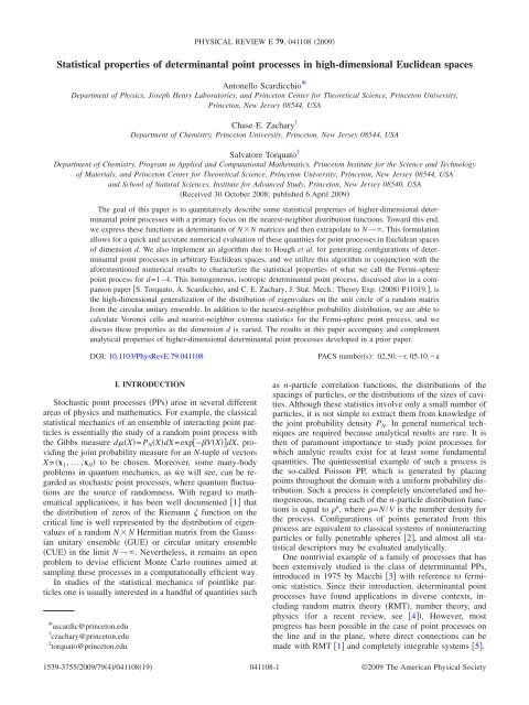
<strong>Statistical</strong> <strong>properties</strong> <strong>of</strong> <strong>determ<strong>in</strong>antal</strong> <strong>po<strong>in</strong>t</strong> <strong>processes</strong> <strong>in</strong> <strong>high</strong>-dimensional Euclidean spaces<br />
Antonello Scardicchio*<br />
Department <strong>of</strong> Physics, Joseph Henry Laboratories, and Pr<strong>in</strong>ceton Center for Theoretical Science, Pr<strong>in</strong>ceton University,<br />
Pr<strong>in</strong>ceton, New Jersey 08544, USA<br />
Chase E. Zachary †<br />
Department <strong>of</strong> Chemistry, Pr<strong>in</strong>ceton University, Pr<strong>in</strong>ceton, New Jersey 08544, USA<br />
Salvatore Torquato ‡<br />
Department <strong>of</strong> Chemistry, Program <strong>in</strong> Applied and Computational Mathematics, Pr<strong>in</strong>ceton Institute for the Science and Technology<br />
<strong>of</strong> Materials, and Pr<strong>in</strong>ceton Center for Theoretical Science, Pr<strong>in</strong>ceton University, Pr<strong>in</strong>ceton, New Jersey 08544, USA<br />
and School <strong>of</strong> Natural Sciences, Institute for Advanced Study, Pr<strong>in</strong>ceton, New Jersey 08540, USA<br />
Received 30 October 2008; published 6 April 2009<br />
The goal <strong>of</strong> this paper is to quantitatively describe some statistical <strong>properties</strong> <strong>of</strong> <strong>high</strong>er-dimensional <strong>determ<strong>in</strong>antal</strong><br />
<strong>po<strong>in</strong>t</strong> <strong>processes</strong> with a primary focus on the nearest-neighbor distribution functions. Toward this end,<br />
we express these functions as determ<strong>in</strong>ants <strong>of</strong> NN matrices and then extrapolate to N→. This formulation<br />
allows for a quick and accurate numerical evaluation <strong>of</strong> these quantities for <strong>po<strong>in</strong>t</strong> <strong>processes</strong> <strong>in</strong> Euclidean spaces<br />
<strong>of</strong> dimension d. We also implement an algorithm due to Hough et al. for generat<strong>in</strong>g configurations <strong>of</strong> <strong>determ<strong>in</strong>antal</strong><br />
<strong>po<strong>in</strong>t</strong> <strong>processes</strong> <strong>in</strong> arbitrary Euclidean spaces, and we utilize this algorithm <strong>in</strong> conjunction with the<br />
aforementioned numerical results to characterize the statistical <strong>properties</strong> <strong>of</strong> what we call the Fermi-sphere<br />
<strong>po<strong>in</strong>t</strong> process for d=1–4. This homogeneous, isotropic <strong>determ<strong>in</strong>antal</strong> <strong>po<strong>in</strong>t</strong> process, discussed also <strong>in</strong> a companion<br />
paper S. Torquato, A. Scardicchio, and C. E. Zachary, J. Stat. Mech.: Theory Exp. 2008 P11019., is<br />
the <strong>high</strong>-dimensional generalization <strong>of</strong> the distribution <strong>of</strong> eigenvalues on the unit circle <strong>of</strong> a random matrix<br />
from the circular unitary ensemble. In addition to the nearest-neighbor probability distribution, we are able to<br />
calculate Voronoi cells and nearest-neighbor extrema statistics for the Fermi-sphere <strong>po<strong>in</strong>t</strong> process, and we<br />
discuss these <strong>properties</strong> as the dimension d is varied. The results <strong>in</strong> this paper accompany and complement<br />
analytical <strong>properties</strong> <strong>of</strong> <strong>high</strong>er-dimensional <strong>determ<strong>in</strong>antal</strong> <strong>po<strong>in</strong>t</strong> <strong>processes</strong> developed <strong>in</strong> a prior paper.<br />
DOI: 10.1103/PhysRevE.79.041108 PACS numbers: 02.50.r, 05.10.a<br />
I. INTRODUCTION<br />
Stochastic <strong>po<strong>in</strong>t</strong> <strong>processes</strong> PPs arise <strong>in</strong> several different<br />
areas <strong>of</strong> physics and mathematics. For example, the classical<br />
statistical mechanics <strong>of</strong> an ensemble <strong>of</strong> <strong>in</strong>teract<strong>in</strong>g <strong>po<strong>in</strong>t</strong> particles<br />
is essentially the study <strong>of</strong> a random <strong>po<strong>in</strong>t</strong> process with<br />
the Gibbs measure dX= P NXdX=exp−VXdX, provid<strong>in</strong>g<br />
the jo<strong>in</strong>t probability measure for an N-tuple <strong>of</strong> vectors<br />
X=x 1,...,x N to be chosen. Moreover, some many-body<br />
problems <strong>in</strong> quantum mechanics, as we will see, can be regarded<br />
as stochastic <strong>po<strong>in</strong>t</strong> <strong>processes</strong>, where quantum fluctuations<br />
are the source <strong>of</strong> randomness. With regard to mathematical<br />
applications, it has been well documented 1 that<br />
the distribution <strong>of</strong> zeros <strong>of</strong> the Riemann function on the<br />
critical l<strong>in</strong>e is well represented by the distribution <strong>of</strong> eigenvalues<br />
<strong>of</strong> a random NN Hermitian matrix from the Gaussian<br />
unitary ensemble GUE or circular unitary ensemble<br />
CUE <strong>in</strong> the limit N→. Nevertheless, it rema<strong>in</strong>s an open<br />
problem to devise efficient Monte Carlo rout<strong>in</strong>es aimed at<br />
sampl<strong>in</strong>g these <strong>processes</strong> <strong>in</strong> a computationally efficient way.<br />
In studies <strong>of</strong> the statistical mechanics <strong>of</strong> <strong>po<strong>in</strong>t</strong>like particles<br />
one is usually <strong>in</strong>terested <strong>in</strong> a handful <strong>of</strong> quantities such<br />
*ascardic@pr<strong>in</strong>ceton.edu<br />
† czachary@pr<strong>in</strong>ceton.edu<br />
‡ torquato@pr<strong>in</strong>ceton.edu<br />
PHYSICAL REVIEW E 79, 041108 2009<br />
as n-particle correlation functions, the distributions <strong>of</strong> the<br />
spac<strong>in</strong>gs <strong>of</strong> particles, or the distributions <strong>of</strong> the sizes <strong>of</strong> cavities.<br />
Although these statistics <strong>in</strong>volve only a small number <strong>of</strong><br />
particles, it is not simple to extract them from knowledge <strong>of</strong><br />
the jo<strong>in</strong>t probability density P N. In general numerical techniques<br />
are required because analytical results are rare. It is<br />
then <strong>of</strong> paramount importance to study <strong>po<strong>in</strong>t</strong> <strong>processes</strong> for<br />
which analytic results exist for at least some fundamental<br />
quantities. The qu<strong>in</strong>tessential example <strong>of</strong> such a process is<br />
the so-called Poisson PP, which is generated by plac<strong>in</strong>g<br />
<strong>po<strong>in</strong>t</strong>s throughout the doma<strong>in</strong> with a uniform probability distribution.<br />
Such a process is completely uncorrelated and homogeneous,<br />
mean<strong>in</strong>g each <strong>of</strong> the n-particle distribution functions<br />
is equal to n , where =N/V is the number density for<br />
the process. Configurations <strong>of</strong> <strong>po<strong>in</strong>t</strong>s generated from this<br />
process are equivalent to classical systems <strong>of</strong> non<strong>in</strong>teract<strong>in</strong>g<br />
particles or fully penetrable spheres 2, and almost all statistical<br />
descriptors may be evaluated analytically.<br />
One nontrivial example <strong>of</strong> a family <strong>of</strong> <strong>processes</strong> that has<br />
been extensively studied is the class <strong>of</strong> <strong>determ<strong>in</strong>antal</strong> PPs,<br />
<strong>in</strong>troduced <strong>in</strong> 1975 by Macchi 3 with reference to fermionic<br />
statistics. S<strong>in</strong>ce their <strong>in</strong>troduction, <strong>determ<strong>in</strong>antal</strong> <strong>po<strong>in</strong>t</strong><br />
<strong>processes</strong> have found applications <strong>in</strong> diverse contexts, <strong>in</strong>clud<strong>in</strong>g<br />
random matrix theory RMT, number theory, and<br />
physics for a recent review, see 4. However, most<br />
progress has been possible <strong>in</strong> the case <strong>of</strong> <strong>po<strong>in</strong>t</strong> <strong>processes</strong> on<br />
the l<strong>in</strong>e and <strong>in</strong> the plane, where direct connections can be<br />
made with RMT 1 and completely <strong>in</strong>tegrable systems 5.<br />
1539-3755/2009/794/04110819 041108-1<br />
©2009 The American Physical Society
SCARDICCHIO, ZACHARY, AND TORQUATO PHYSICAL REVIEW E 79, 041108 2009<br />
Similar connections have not yet been found, to the best<br />
<strong>of</strong> our knowledge, for <strong>high</strong>er-dimensional <strong>determ<strong>in</strong>antal</strong><br />
<strong>po<strong>in</strong>t</strong> <strong>processes</strong>, and numerical and analytical results <strong>in</strong> dimension<br />
d3 are miss<strong>in</strong>g altogether. In this paper and its<br />
companion 6, we provide a generalization <strong>of</strong> these <strong>po<strong>in</strong>t</strong><br />
<strong>processes</strong> to <strong>high</strong>er dimensions, which we call Fermi-sphere<br />
<strong>po<strong>in</strong>t</strong> <strong>processes</strong>. While <strong>in</strong> 6 we have studied, ma<strong>in</strong>ly by<br />
way <strong>of</strong> exact analyses, statistical descriptors such as<br />
n-particle probability densities and nearest-neighbor functions<br />
for these <strong>po<strong>in</strong>t</strong> <strong>processes</strong>, here we base most <strong>of</strong> our<br />
analysis on an efficient algorithm 7 for generat<strong>in</strong>g configurations<br />
from arbitrary <strong>determ<strong>in</strong>antal</strong> <strong>po<strong>in</strong>t</strong> <strong>processes</strong> and are<br />
therefore able to study other particle and void statistics related<br />
to nearest-neighbor distributions and Voronoi cells.<br />
In particular, after present<strong>in</strong>g <strong>in</strong> detail our implementation<br />
<strong>of</strong> an algorithm 7 to generate configurations <strong>of</strong> homogenous,<br />
isotropic <strong>determ<strong>in</strong>antal</strong> <strong>po<strong>in</strong>t</strong> <strong>processes</strong>, we study several<br />
statistical quantities there<strong>of</strong>, <strong>in</strong>clud<strong>in</strong>g Voronoi cell statistics<br />
and distributions <strong>of</strong> m<strong>in</strong>imum and maximum nearestneighbor<br />
distances for which no analytical results exist.<br />
Additionally, the large-r behavior <strong>of</strong> the nearest-neighbor<br />
functions is computationally explored. We provide substantial<br />
evidence that the conditional probabilities G P and G V,<br />
def<strong>in</strong>ed below, are asymptotically l<strong>in</strong>ear, and we give estimates<br />
for their slopes as a function <strong>of</strong> dimension d between<br />
one and four.<br />
The plan <strong>of</strong> the paper is as follows. Section II provides a<br />
brief review <strong>of</strong> <strong>determ<strong>in</strong>antal</strong> <strong>po<strong>in</strong>t</strong> <strong>processes</strong> and def<strong>in</strong>es the<br />
statistical quantities used to characterize these systems. Of<br />
particular importance is the formulation <strong>of</strong> the probability<br />
distribution functions govern<strong>in</strong>g nearest-neighbor statistics<br />
as determ<strong>in</strong>ants <strong>of</strong> NN matrices; the results are easily<br />
evaluated numerically. The term<strong>in</strong>ology we develop is then<br />
applied to the statistical <strong>properties</strong> <strong>of</strong> known one- and twodimensional<br />
<strong>determ<strong>in</strong>antal</strong> <strong>po<strong>in</strong>t</strong> <strong>processes</strong> <strong>in</strong> Sec. III. Section<br />
IV discusses the implementation <strong>of</strong> an algorithm for<br />
generat<strong>in</strong>g <strong>determ<strong>in</strong>antal</strong> <strong>po<strong>in</strong>t</strong> <strong>processes</strong> <strong>in</strong> any dimension d,<br />
and we comb<strong>in</strong>e the results from this algorithm and the numerics<br />
<strong>of</strong> Sec. II to characterize the so-called Fermi-sphere<br />
<strong>po<strong>in</strong>t</strong> process for d=1, 2, 3, and 4. In Sec. V we provide an<br />
example <strong>of</strong> a <strong>determ<strong>in</strong>antal</strong> <strong>po<strong>in</strong>t</strong>-process on a curved space<br />
a two-sphere, and our conclusions are collected <strong>in</strong> Sec. VI.<br />
II. FORMALISM OF DETERMINANTAL POINT<br />
PROCESSES<br />
A. Def<strong>in</strong>itions: n-particle correlation functions<br />
Consider N <strong>po<strong>in</strong>t</strong> particles <strong>in</strong> a subset <strong>of</strong> d-dimensional<br />
Euclidean space ER d . It is convenient to <strong>in</strong>troduce the<br />
Hilbert space structure given by square <strong>in</strong>tegrable functions<br />
on E; we will adopt Dirac’s bra-ket notation for these functions.<br />
Unless otherwise specified, all <strong>in</strong>tegrals are <strong>in</strong>tended to<br />
extend over E. A <strong>determ<strong>in</strong>antal</strong> <strong>po<strong>in</strong>t</strong> process can be def<strong>in</strong>ed<br />
as a stochastic <strong>po<strong>in</strong>t</strong> process such that the jo<strong>in</strong>t probability<br />
distribution PN <strong>of</strong> N <strong>po<strong>in</strong>t</strong>s is given as a determ<strong>in</strong>ant <strong>of</strong> a<br />
positive, bounded operator H <strong>of</strong> rank N:<br />
PNx1, ...,xN = 1<br />
N! detHxi,x j1i,jN, 1<br />
where Hx,y is the kernel <strong>of</strong> H. In this paper, we focus on<br />
the simple case <strong>in</strong> which the N nonzero eigenvalues <strong>of</strong> H are<br />
041108-2<br />
all 1; the more general case can be treated with m<strong>in</strong>or<br />
changes 7. We can write down the spectral decomposition<br />
<strong>of</strong> H as<br />
N<br />
H = n=1<br />
0 0<br />
nn, 2<br />
0 N<br />
where nn=1 are the eigenvectors <strong>of</strong> the operator H. The<br />
reason for the superscript on the basis vectors will be clarified<br />
momentarily. The correct normalization <strong>of</strong> the <strong>po<strong>in</strong>t</strong> process<br />
is obta<strong>in</strong>ed easily s<strong>in</strong>ce 1<br />
detHxi,x j1i,jNdx 1 ¯ dxN = N! detH, 3<br />
where the last determ<strong>in</strong>ant is to be <strong>in</strong>terpreted as the product<br />
<strong>of</strong> the nonzero eigenvalues <strong>of</strong> the operator H. S<strong>in</strong>ce these<br />
eigenvalues are all unity we obta<strong>in</strong> detH=1, which yields<br />
P Nx 1, ...,x Ndx 1 ¯ dx N =1. 4<br />
0 N<br />
Notice that <strong>in</strong> terms <strong>of</strong> the basis nn=1 we can also<br />
write<br />
PNx1, ...,xN = 1<br />
N! det 0<br />
i xj1i,jN 2 . 5<br />
An easy pro<strong>of</strong> is obta<strong>in</strong>ed by consider<strong>in</strong>g the square matrix<br />
0<br />
. Then,<br />
0<br />
ij= i xj=x j i<br />
0<br />
deti xj1i,jN 2 = det † det = det † <br />
j<br />
N<br />
0 0<br />
= detxi nnx n=1<br />
= detHxi,x j, 6<br />
which is the same as 1.<br />
Determ<strong>in</strong>antal <strong>po<strong>in</strong>t</strong> <strong>processes</strong> are peculiar <strong>in</strong> that one can<br />
actually write all the n-particle distribution functions explicitly.<br />
The n-particle probability density, denoted by<br />
nx1,...,xn is the generic probability density <strong>of</strong> f<strong>in</strong>d<strong>in</strong>g n<br />
particles <strong>in</strong> volume elements around the given positions<br />
x1,...,xn, irrespective <strong>of</strong> the rema<strong>in</strong><strong>in</strong>g N−n particles. For<br />
a general <strong>determ<strong>in</strong>antal</strong> <strong>po<strong>in</strong>t</strong> process this function takes the<br />
form<br />
nx 1, ...,x n = detHx i,x j 1i,jn. 7<br />
In particular, the s<strong>in</strong>gle-particle probability density is<br />
1x1 = Hx1,x 1. 8<br />
This function is proportional to the probability density <strong>of</strong><br />
f<strong>in</strong>d<strong>in</strong>g a particle at x1, also known as the <strong>in</strong>tensity <strong>of</strong> the<br />
<strong>po<strong>in</strong>t</strong> process. One can see that the normalization is<br />
1xdx =trH = N. 9<br />
For translationally <strong>in</strong>variant <strong>processes</strong> 1x=, <strong>in</strong>dependent<br />
<strong>of</strong> x. We remark <strong>in</strong> pass<strong>in</strong>g that for a f<strong>in</strong>ite system translational<br />
<strong>in</strong>variance is def<strong>in</strong>ed <strong>in</strong> the sense <strong>of</strong> averag<strong>in</strong>g the
STATISTICAL PROPERTIES OF DETERMINANTAL POINT … PHYSICAL REVIEW E 79, 041108 2009<br />
location <strong>of</strong> the orig<strong>in</strong> over R d with periodic boundary conditions<br />
enforced.<br />
It is also possible to write the two-particle probability<br />
density explicitly:<br />
2x 1,x 2 = Hx 1,x 1Hx 2,x 2 − Hx 1,x 2 2 , 10<br />
which has the follow<strong>in</strong>g normalization:<br />
2x 1,x 2dx 1dx 2 = NN −1. 11<br />
In general the normalization for n is given by N!/N−n!,<br />
or the number <strong>of</strong> ways <strong>of</strong> choos<strong>in</strong>g an ordered subset <strong>of</strong> n<br />
<strong>po<strong>in</strong>t</strong>s from a population <strong>of</strong> size N. For a translationally <strong>in</strong>variant<br />
and completely uncorrelated <strong>po<strong>in</strong>t</strong> process 10 simplifies<br />
accord<strong>in</strong>g to 2= 2 .<br />
We also <strong>in</strong>troduce the n-particle correlation functions gn, which are def<strong>in</strong>ed by<br />
gnx1, ...,xn = nx1, ...,xn n . 12<br />
S<strong>in</strong>ce n= n for a completely uncorrelated <strong>po<strong>in</strong>t</strong> process, it<br />
follows that deviations <strong>of</strong> g n from unity provide a measure <strong>of</strong><br />
the correlations between <strong>po<strong>in</strong>t</strong>s <strong>in</strong> a <strong>po<strong>in</strong>t</strong> process. Of particular<br />
<strong>in</strong>terest is the pair correlation function, which for a<br />
translationally <strong>in</strong>variant <strong>po<strong>in</strong>t</strong> process <strong>of</strong> <strong>in</strong>tensity can be<br />
written as<br />
g 2x 1,x 2 = 2x 1,x 2<br />
2<br />
=1− Hx 2<br />
1,x2 . 13<br />
<br />
Closely related to the pair correlation function is the total<br />
correlation function, denoted by h; it is derived from g 2 via<br />
the equation<br />
hx,y = g 2x,y −1=− −2 Hx,y 2 , 14<br />
where the second equality applies for all <strong>determ<strong>in</strong>antal</strong> <strong>po<strong>in</strong>t</strong><br />
<strong>processes</strong> by 13. S<strong>in</strong>ce g 2r→1 asr→ r=x−y for<br />
translationally <strong>in</strong>variant systems without long-range order, it<br />
follows that hr→0 <strong>in</strong> this limit, mean<strong>in</strong>g that h is generally<br />
an L 2 function, and its Fourier transform is well def<strong>in</strong>ed.<br />
Determ<strong>in</strong>antal <strong>po<strong>in</strong>t</strong> <strong>processes</strong> are self-similar; <strong>in</strong>tegration<br />
<strong>of</strong> the n-particle probability distribution with respect to a<br />
<strong>po<strong>in</strong>t</strong> gives back the same functional form. 1 This property is<br />
desirable s<strong>in</strong>ce it considerably simplifies the computation <strong>of</strong><br />
many quantities. However, we note that even complete<br />
knowledge <strong>of</strong> all the n-particle probability distributions is<br />
not sufficient <strong>in</strong> practice to generate <strong>po<strong>in</strong>t</strong> <strong>processes</strong> from the<br />
given probability P N. This notoriously difficult issue is<br />
known as the reconstruction problem <strong>in</strong> statistical mechanics<br />
8–11. When <strong>in</strong> Sec. IV we discuss an explicit constructive<br />
algorithm to generate realizations <strong>of</strong> a given <strong>determ<strong>in</strong>antal</strong><br />
process, the reader should keep <strong>in</strong> m<strong>in</strong>d that the ability to<br />
1 One could th<strong>in</strong>k <strong>in</strong> terms <strong>of</strong> effective <strong>in</strong>teractions and renormalization<br />
group. The <strong>determ<strong>in</strong>antal</strong> form <strong>of</strong> the probabilities n then is<br />
a fixed <strong>po<strong>in</strong>t</strong> <strong>of</strong> the renormalization operation <strong>of</strong> <strong>in</strong>tegrat<strong>in</strong>g out one<br />
or more particles.<br />
041108-3<br />
write down all the n-particle correlation functions g n is not<br />
the reason why there exists such a constructive algorithm.<br />
B. Exact results for some statistical quantities<br />
We have seen that the <strong>determ<strong>in</strong>antal</strong> form <strong>of</strong> the probability<br />
density function allows us to write down all n-particle<br />
correlation functions gn <strong>in</strong> a quick and simple manner. However,<br />
we can also express more <strong>in</strong>terest<strong>in</strong>g functions, such as<br />
the probability <strong>of</strong> hav<strong>in</strong>g an empty region D or the expected<br />
number <strong>of</strong> <strong>po<strong>in</strong>t</strong>s <strong>in</strong> a given region, as properly constructed<br />
determ<strong>in</strong>ants <strong>of</strong> the operator H. This property has been used<br />
<strong>in</strong> random matrix theory to f<strong>in</strong>d the exact gap distribution <strong>of</strong><br />
eigenvalues on the l<strong>in</strong>e <strong>in</strong> terms <strong>of</strong> solutions <strong>of</strong> a nonl<strong>in</strong>ear<br />
differential equation 12. The relevant formula is a special<br />
case <strong>of</strong> the result 4 that the generat<strong>in</strong>g function <strong>of</strong> the distribution<br />
<strong>of</strong> the number <strong>po<strong>in</strong>t</strong>s nD <strong>in</strong> the region D is<br />
znD = PnD = nz<br />
n0<br />
n = detI + z −1DHD, 15<br />
where D is the characteristic function <strong>of</strong> D, I is the identity<br />
operator, and zR. We will also denote Pn PnD=n. Therefore, the probability that the region D is empty is obta<strong>in</strong>ed<br />
by tak<strong>in</strong>g the limit z→0 <strong>in</strong> the previous formula. The<br />
result is<br />
P 0 = detI − DH D. 16<br />
Equation 16 may be written more explicitly. Consider the<br />
eigenvalues i <strong>of</strong> DH D. By the def<strong>in</strong>ition <strong>of</strong> the determ<strong>in</strong>ant,<br />
Eq. 16 takes the form<br />
N<br />
P 0 = i=1<br />
1− i, 17<br />
where the product is over the nonzero eigenvalues <strong>of</strong> DHD only <strong>of</strong> which there are N, the number <strong>of</strong> particles. First<br />
notice that for the nonzero i we have i= ˜ i, where ˜ N<br />
ii=1 are the N eigenvalues <strong>of</strong> H DH. In fact one can show that<br />
the traces <strong>of</strong> all the powers <strong>of</strong> these two operators are the<br />
same us<strong>in</strong>g D 2 =D,H 2 =H, and the cyclic property <strong>of</strong> the<br />
trace operation. This condition is sufficient for N f<strong>in</strong>ite, and<br />
the limit N→ can be taken afterward. The operator HDH N<br />
can now be written <strong>in</strong> a basis nn=1 as the matrix<br />
and the determ<strong>in</strong>ant <strong>in</strong> 16 as<br />
MijD = ix jxdx, 18<br />
D<br />
P0 = detij − Mij. 19<br />
We will be us<strong>in</strong>g this formula <strong>of</strong>ten <strong>in</strong> the follow<strong>in</strong>g analysis.<br />
The probability P0 has a unique role <strong>in</strong> the study <strong>of</strong> various<br />
<strong>po<strong>in</strong>t</strong> <strong>processes</strong> 2, <strong>in</strong> particular when D=B0;r, a ball <strong>of</strong><br />
radius r for translationally <strong>in</strong>variant <strong>processes</strong> the position<br />
<strong>of</strong> the center <strong>of</strong> the ball is immaterial. In this context, P0 is<br />
called the void exclusion probability EVr 2,13–15, and we<br />
will adopt this name and notation <strong>in</strong> this paper <strong>in</strong> 6 we<br />
have studied this quantity <strong>in</strong> an appropriate scal<strong>in</strong>g limit,<br />
when d→.
SCARDICCHIO, ZACHARY, AND TORQUATO PHYSICAL REVIEW E 79, 041108 2009<br />
However, there are statistical quantities <strong>of</strong> great importance<br />
which cannot be found with the above formalism. For<br />
example, one can exam<strong>in</strong>e the distribution <strong>of</strong> the maximum<br />
or m<strong>in</strong>imum nearest-neighbor distances <strong>in</strong> a <strong>determ<strong>in</strong>antal</strong><br />
<strong>po<strong>in</strong>t</strong> process, or the “extremum statistics,” and these quantities<br />
cannot be found easily by the above means. One could<br />
also explore the distribution <strong>of</strong> the Voronoi cell statistics or<br />
the percolation threshold for the PP. To determ<strong>in</strong>e these<br />
quantities we will have to rely on an explicit realization <strong>of</strong> a<br />
<strong>determ<strong>in</strong>antal</strong> <strong>po<strong>in</strong>t</strong> process. The existence and the analysis<br />
<strong>of</strong> an algorithm to perform this task is a central topic <strong>of</strong> this<br />
paper.<br />
We <strong>in</strong>troduce now some quantities which characterize a<br />
PP 2,13–15. We start with the above expression E Vr for<br />
the probability <strong>of</strong> f<strong>in</strong>d<strong>in</strong>g a spherical cavity <strong>of</strong> radius r <strong>in</strong> the<br />
<strong>po<strong>in</strong>t</strong> process. Analogously, one can def<strong>in</strong>e the probability <strong>of</strong><br />
f<strong>in</strong>d<strong>in</strong>g a spherical cavity <strong>of</strong> radius r centered on a <strong>po<strong>in</strong>t</strong> <strong>of</strong><br />
the process, which we denote as E Pr. E P can be found <strong>in</strong><br />
connection with E V us<strong>in</strong>g the follow<strong>in</strong>g construction. Consider<br />
the probability <strong>of</strong> f<strong>in</strong>d<strong>in</strong>g no <strong>po<strong>in</strong>t</strong>s <strong>in</strong> the spherical<br />
shell <strong>of</strong> <strong>in</strong>ner radius and outer radius r, which we call<br />
E Vr;. This function can be obta<strong>in</strong>ed by either <strong>of</strong> the previous<br />
formulas 16 or 19. It is clear that E Vr=E Vr;0. It<br />
is also true that for sufficiently small the probability <strong>of</strong><br />
hav<strong>in</strong>g two or more <strong>po<strong>in</strong>t</strong>s <strong>in</strong> the sphere <strong>of</strong> radius is negligibly<br />
small compared to the probability <strong>of</strong> hav<strong>in</strong>g one particle.<br />
Hence, the probability r; <strong>of</strong> f<strong>in</strong>d<strong>in</strong>g no particles <strong>in</strong><br />
the spherical shell B0;r\B0; conditioned on the presence<br />
<strong>of</strong> one <strong>po<strong>in</strong>t</strong> <strong>in</strong> a sphere <strong>of</strong> radius and volume v is<br />
r; = EVr; − EVr;0 , 20<br />
v<br />
and by tak<strong>in</strong>g the limit →0 <strong>of</strong> this expression we f<strong>in</strong>d that<br />
EPr = lim r;. 21<br />
→0<br />
That E P0=1 can be seen from the follow<strong>in</strong>g argument. Set<br />
r=+0 + . Then E V+0 + ;=1 because the region is <strong>in</strong>f<strong>in</strong>itesimal<br />
and hence empty with probability 1, and E V;0<br />
1−v s<strong>in</strong>ce for sufficiently small we have at most one<br />
<strong>po<strong>in</strong>t</strong> <strong>in</strong> the region. One l<strong>in</strong>e <strong>of</strong> algebra provides the result.<br />
Us<strong>in</strong>g this expression, we can derive an <strong>in</strong>terest<strong>in</strong>g and<br />
practical result for E P. First, notice that E Vr; conta<strong>in</strong>s the<br />
matrix M ijr; def<strong>in</strong>ed by 18, which when →0 becomes<br />
M ijr;M ijr − v i0 j0. 22<br />
Moreover, if we assume that I−M is <strong>in</strong>vertible, we can see<br />
that to first order <strong>in</strong> M<br />
detI − M + M = expln detI − M + M<br />
= exptrlnI − M + M<br />
exptrlnI − M +trMI− M−1 detI − M1+trMI− M−1. 23<br />
From 23 we f<strong>in</strong>d the f<strong>in</strong>al result:<br />
041108-4<br />
E Pr = E VrtrAI − M −1 , 24<br />
where Aij= i0 j0/. Notice that for r→0 we have M<br />
→0, and EP0=trA=ii02 /=H0,0/=1 as expected.<br />
These two primary functions can be used to def<strong>in</strong>e four<br />
other quantities <strong>of</strong> <strong>in</strong>terest. Two are density functions,<br />
HVr =− EVr , 25<br />
r<br />
HPr =− EPr , 26<br />
r<br />
which can be <strong>in</strong>terpreted as the probability densities <strong>of</strong> f<strong>in</strong>d<strong>in</strong>g<br />
the closest particle at distance r from a random <strong>po<strong>in</strong>t</strong> <strong>of</strong><br />
the space or another random <strong>po<strong>in</strong>t</strong> <strong>of</strong> the process, respectively.<br />
The other two functions are conditional probabilities,<br />
GVr = HVr , 27<br />
srEVr GPr = HPr , 28<br />
srEPr which give the density <strong>of</strong> <strong>po<strong>in</strong>t</strong>s around a spherical cavity<br />
centered, respectively, on a random <strong>po<strong>in</strong>t</strong> <strong>of</strong> the space or on<br />
a random <strong>po<strong>in</strong>t</strong> <strong>of</strong> the process. We note that sr is the surface<br />
area <strong>of</strong> the d-dimensional sphere <strong>of</strong> radius r. We will<br />
study the behavior <strong>of</strong> these functions for some <strong>determ<strong>in</strong>antal</strong><br />
PPs <strong>in</strong> Secs. III and IV <strong>of</strong> this paper.<br />
From the def<strong>in</strong>itions <strong>in</strong> 25–28 <strong>in</strong> conjunction with 19<br />
and 24, it is possible to express HV, HP, GV, and GP as<br />
numerically solvable operations on NN matrices. The results<br />
are<br />
H Vr = E VrtrI − M −1M<br />
r , 29<br />
H Pr = H VrtrAI − M −1 <br />
− E VrtrAI − M −1M<br />
r I − M−1, 30<br />
G Vr = 1<br />
srtrI − M −1M<br />
r , 31<br />
GPr = GVr − 1<br />
sr <br />
r ln trAI − M−1. 32<br />
The form G Pr=G Vr−G ˜ r which serves as a def<strong>in</strong>ition<br />
<strong>of</strong> G ˜ <strong>in</strong> 32 is <strong>of</strong> particular <strong>in</strong>terest. If the correction term<br />
G ˜ r0 for all r, positivity and monotonicity <strong>of</strong> G P which<br />
must be proven <strong>in</strong>dependently are then sufficient to ensure<br />
that, for appropriately large r, G PrG Vr <strong>in</strong> scal<strong>in</strong>g. Although<br />
we have been unable to develop analytic results for<br />
the large-r behavior <strong>of</strong> G ˜ , numerical results, which are provided<br />
later see Fig. 10, suggest that G ˜ 0 and G ˜ →0 monotonically<br />
as r→ for d2, and G ˜ →constant for d=1. As
STATISTICAL PROPERTIES OF DETERMINANTAL POINT … PHYSICAL REVIEW E 79, 041108 2009<br />
E p (r)<br />
1<br />
0.9<br />
0.8<br />
0.7<br />
0.6<br />
0.5<br />
0.4<br />
0.3<br />
0.2<br />
0.1<br />
N=5<br />
N=50<br />
N = 100<br />
0<br />
0 0.2 0.4 0.6 0.8 1 1.2 1.4 1.6 1.8 2<br />
r<br />
FIG. 1. Color onl<strong>in</strong>e Convergence <strong>of</strong> the d=1 numerical results<br />
us<strong>in</strong>g 19 for E P with respect to <strong>in</strong>creas<strong>in</strong>g matrix size N.<br />
both behaviors are subdom<strong>in</strong>ant with respect to the l<strong>in</strong>ear<br />
growth <strong>of</strong> G V, we expect that G P and G V possess the same<br />
l<strong>in</strong>ear slope for sufficiently large r.<br />
An important <strong>po<strong>in</strong>t</strong> to address is the convergence <strong>of</strong> the<br />
results from 19 <strong>in</strong> the limit N→. We expect that the calculations<br />
for f<strong>in</strong>ite but large N provide an <strong>in</strong>creas<strong>in</strong>gly sharp<br />
approximation to the results from the N→ limit. Figure 1<br />
presents the calculation <strong>of</strong> E P for a few values <strong>of</strong> N with d<br />
=1; it is clear that the numerical calculations quickly approach<br />
a fixed function for N40, and it is this function<br />
which we accept as the correct large-N limit. The results for<br />
<strong>high</strong>er-dimensional <strong>processes</strong> are similar, and we will assume<br />
that this convergence property holds throughout the<br />
rema<strong>in</strong>der <strong>of</strong> the paper.<br />
C. Hyperuniformity <strong>of</strong> <strong>po<strong>in</strong>t</strong> <strong>processes</strong><br />
Of particular significance <strong>in</strong> understand<strong>in</strong>g the <strong>properties</strong><br />
<strong>of</strong> <strong>determ<strong>in</strong>antal</strong> <strong>po<strong>in</strong>t</strong> <strong>processes</strong> is the notion <strong>of</strong> hyperuniformity,<br />
also known as superhomogeneity. A hyperuniform<br />
<strong>po<strong>in</strong>t</strong> pattern is a system <strong>of</strong> <strong>po<strong>in</strong>t</strong>s such that the variance<br />
2 2<br />
R=N R−NR<br />
2 <strong>of</strong> the number <strong>of</strong> <strong>po<strong>in</strong>t</strong>s NR <strong>in</strong> a spherical<br />
w<strong>in</strong>dow <strong>of</strong> radius R obey<br />
2 RR d−1 33<br />
for large R 8. This condition <strong>in</strong> turn implies that the structure<br />
factor Sk=1+h ˆ k has the follow<strong>in</strong>g small-k behavior:<br />
lim Sk =0, 34<br />
k→0<br />
mean<strong>in</strong>g that hyperuniform <strong>po<strong>in</strong>t</strong> patterns do not possess<br />
<strong>in</strong>f<strong>in</strong>ite-wavelength number fluctuations 8. Examples <strong>of</strong> hyperuniform<br />
systems <strong>in</strong>clude all periodic <strong>po<strong>in</strong>t</strong> <strong>processes</strong> 8,<br />
certa<strong>in</strong> aperiodic <strong>po<strong>in</strong>t</strong> <strong>processes</strong> 8,16, one-component<br />
plasmas 8,16, <strong>po<strong>in</strong>t</strong> <strong>processes</strong> associated with a wide class<br />
<strong>of</strong> til<strong>in</strong>gs <strong>of</strong> space 17,18, and certa<strong>in</strong> disordered sphere<br />
pack<strong>in</strong>gs 6,9,19,20. It has also been shown 6 that the<br />
Fermi-sphere <strong>determ<strong>in</strong>antal</strong> <strong>po<strong>in</strong>t</strong> process, described below,<br />
is hyperuniform.<br />
041108-5<br />
The condition <strong>in</strong> 34 suggests that for general translationally<br />
<strong>in</strong>variant nonperiodic systems<br />
Skk k → 0 35<br />
for some 0. However, hyperuniform <strong>determ<strong>in</strong>antal</strong> <strong>po<strong>in</strong>t</strong><br />
<strong>processes</strong> may exhibit only certa<strong>in</strong> scal<strong>in</strong>g exponents . One<br />
can see for a <strong>determ<strong>in</strong>antal</strong> <strong>po<strong>in</strong>t</strong> process that<br />
Sk =1−FH 2 k, 36<br />
where F denotes the Fourier transform and we have without<br />
loss <strong>of</strong> generality set =1. Equation 36 therefore suggests<br />
that<br />
FH 2 k1−k k → 0. 37<br />
Tak<strong>in</strong>g the <strong>in</strong>verse Fourier transform <strong>of</strong> 37 gives the follow<strong>in</strong>g<br />
large-r scal<strong>in</strong>g <strong>of</strong> Hr 2 :<br />
Hr2 − 1<br />
d/22 + d 2<br />
r+d− <br />
2 r<br />
→ . 38<br />
The negative coefficient and the negative argument <strong>of</strong> the<br />
Gamma function <strong>in</strong> 38 are crucially important. S<strong>in</strong>ce<br />
Hr 2 0 for all r, it must be true that −/20, and this<br />
condition restricts the possible values <strong>of</strong> the scal<strong>in</strong>g exponent<br />
. Namely, the behavior <strong>of</strong> the Gamma function requires that<br />
fall <strong>in</strong>to one <strong>of</strong> the <strong>in</strong>tervals 0, 2, 4, 6, 8, 10, and so<br />
forth. We remark that the <strong>in</strong>teger-valued end <strong>po<strong>in</strong>t</strong>s <strong>of</strong> these<br />
<strong>in</strong>tervals are <strong>in</strong>deed valid choices for and imply that<br />
Hr0 for sufficiently large r. These values <strong>of</strong> are<br />
therefore types <strong>of</strong> “limit<strong>in</strong>g values” that overcome the otherwise<br />
dom<strong>in</strong>ant r −+d asymptotic scal<strong>in</strong>g <strong>of</strong> Hr 2 . We provide<br />
an example <strong>of</strong> a <strong>determ<strong>in</strong>antal</strong> <strong>po<strong>in</strong>t</strong> process with the<br />
critical scal<strong>in</strong>g =2 <strong>in</strong> Sec. III C; the result<strong>in</strong>g large-r behavior<br />
for Hr is seen to be Gaussian.<br />
III. PROPERTIES OF KNOWN DETERMINANTAL POINT<br />
PROCESSES<br />
A. One-dimensional <strong>processes</strong><br />
By far the most widely studied examples <strong>of</strong> <strong>determ<strong>in</strong>antal</strong><br />
<strong>po<strong>in</strong>t</strong> <strong>processes</strong> are <strong>in</strong> one dimension. In fact, the connection<br />
to RMT led others to explore the statistical <strong>properties</strong> <strong>of</strong><br />
these systems even prior to the formal <strong>in</strong>troduction <strong>of</strong> <strong>determ<strong>in</strong>antal</strong><br />
<strong>po<strong>in</strong>t</strong> <strong>processes</strong>. To make this connection explicit,<br />
consider an NN random Gaussian Hermitian matrix, i.e., a<br />
matrix whose elements are <strong>in</strong>dependent random numbers distributed<br />
accord<strong>in</strong>g to a normal distribution. This class <strong>of</strong> matrices<br />
def<strong>in</strong>es the Gaussian unitary ensemble. It is possible to<br />
see 1 that the distribution <strong>in</strong>duced on the eigenvalues <strong>of</strong><br />
these random matrices is<br />
N1, ...,N = 1<br />
i − j ZN ij<br />
2 exp− <br />
i<br />
2 i , 39<br />
where Z N is an appropriate normalization constant. By a<br />
standard identity for the Vandermonde determ<strong>in</strong>ant,
SCARDICCHIO, ZACHARY, AND TORQUATO PHYSICAL REVIEW E 79, 041108 2009<br />
i − j ij<br />
2 n<br />
= deti 1i,nN2 , 40<br />
and by comb<strong>in</strong><strong>in</strong>g the rows <strong>of</strong> the matrix i n appropriately we<br />
f<strong>in</strong>d<br />
i − j ij<br />
2 = detHji1i,jN 2 , 41<br />
where the functions Hnx are the Hermite orthogonal polynomials<br />
normalized such that the coefficient <strong>of</strong> the <strong>high</strong>est<br />
power xn <strong>of</strong> Hn is unity. Tak<strong>in</strong>g <strong>in</strong>to account the weight e−x2, we can write <strong>in</strong> agreement with 5<br />
pN = 1<br />
N! detji1ijN 2 , 42<br />
where the orthonormal basis set is<br />
nx = 1<br />
H<br />
z<br />
nxexp− x<br />
n<br />
2 /2; 43<br />
z n is a normalization factor. Therefore, this distribution is<br />
equivalent to the one <strong>in</strong>duced by a system <strong>of</strong> non<strong>in</strong>teract<strong>in</strong>g,<br />
sp<strong>in</strong>less fermions <strong>in</strong> a harmonic potential. We note without<br />
pro<strong>of</strong> that the other canonical random matrix ensembles<br />
Gaussian Orthogonal Ensemble and Gaussian Symplectic<br />
Ensemble can also be expressed as <strong>determ<strong>in</strong>antal</strong> <strong>po<strong>in</strong>t</strong> <strong>processes</strong><br />
by <strong>in</strong>troduc<strong>in</strong>g an <strong>in</strong>ternal vector <strong>in</strong>dex for the basis<br />
functions 1,4.<br />
Another prom<strong>in</strong>ent example <strong>of</strong> a d=1 <strong>determ<strong>in</strong>antal</strong> <strong>po<strong>in</strong>t</strong><br />
process is given by the unitary matrices distributed accord<strong>in</strong>g<br />
to the <strong>in</strong>variant Haar measure; the result<strong>in</strong>g class is termed<br />
the circular unitary ensemble 21. The eigenvalues <strong>of</strong> these<br />
matrices can be written <strong>in</strong> the form j=e i j with j<br />
0,2 ∀ jN; they are distributed accord<strong>in</strong>g to 5 with<br />
the basis<br />
n = 1<br />
exp<strong>in</strong>. 44<br />
2<br />
Notice that the eigenvalues represent the positions <strong>of</strong> free<br />
fermions on a circle, where the Fermi sphere has been filled<br />
cont<strong>in</strong>uously from momentum 0 to N−1.<br />
Another possible one-dimensional process is obta<strong>in</strong>ed by<br />
chang<strong>in</strong>g the exponent x2 <strong>in</strong> 39 to an arbitrary polynomial.<br />
This generalization has <strong>in</strong>terest<strong>in</strong>g connections to the comb<strong>in</strong>atorics<br />
<strong>of</strong> Feynman diagrams and to random polygonizations<br />
<strong>of</strong> surfaces 22. For other examples <strong>of</strong> onedimensional<br />
<strong>determ<strong>in</strong>antal</strong> <strong>po<strong>in</strong>t</strong> <strong>processes</strong>, we refer the<br />
reader to 4.<br />
B. Exact results <strong>in</strong> one dimension<br />
For historical reasons, the most studied descriptor <strong>of</strong> <strong>determ<strong>in</strong>antal</strong><br />
<strong>po<strong>in</strong>t</strong> <strong>processes</strong> is the gap distribution function,<br />
which represents the probability density <strong>of</strong> f<strong>in</strong>d<strong>in</strong>g a chord <strong>of</strong><br />
length s separat<strong>in</strong>g two <strong>po<strong>in</strong>t</strong>s <strong>in</strong> the system for d=1; we<br />
denote this function by ps. For canonical ensembles <strong>of</strong> random<br />
matrices exact solutions for ps have been written <strong>in</strong><br />
terms <strong>of</strong> solutions <strong>of</strong> well-known nonl<strong>in</strong>ear differential equations<br />
1. We start with the follow<strong>in</strong>g observation: after an<br />
041108-6<br />
appropriate rescal<strong>in</strong>g <strong>of</strong> the eigenvalues, the gap distribution<br />
<strong>of</strong> eigenvalues <strong>of</strong> a random matrix is a universal function,<br />
depend<strong>in</strong>g only on the “nature” <strong>of</strong> the ensemble unitary,<br />
orthogonal or symplectic which def<strong>in</strong>es the small-r behavior<br />
<strong>of</strong> g2. For example, the two ensembles the GUE and CUE<br />
def<strong>in</strong>ed above will have the same gap distribution <strong>in</strong> the limit<br />
N→. In the case <strong>of</strong> the GUE the limit is taken for the<br />
eigenvalues<br />
i = z + <br />
2N yi, 45<br />
where z is <strong>in</strong> the “bulk” <strong>of</strong> the distribution z2N− for<br />
N large. One can prove that all the eigenvalues <strong>of</strong> a large<br />
random matrix will fall <strong>in</strong> an <strong>in</strong>terval <strong>of</strong> size 22N with<br />
probability 1 <strong>in</strong> the large-N limit. After this rescal<strong>in</strong>g, the<br />
kernel H converges to the “s<strong>in</strong>e kernel” <strong>in</strong> the large-N limit<br />
12,23:<br />
H N 1, 2 ——→<br />
N→<br />
Hy1,y 2 = s<strong>in</strong>y1 − y2 . 46<br />
y1 − y2 From this result one can f<strong>in</strong>d the n-particle correlation functions.<br />
In particular, one f<strong>in</strong>ds for g 2<br />
2<br />
s<strong>in</strong>x − y<br />
g2x,y =1− . 47<br />
x − y<br />
Application <strong>of</strong> this procedure to the CUE leads to the very<br />
same kernel; for a wider class <strong>of</strong> examples relevant to physics,<br />
see 24. Convergence <strong>of</strong> the kernel implies weak convergence<br />
<strong>of</strong> all the n-particle correlation functions to universal<br />
distributions. These distributions are def<strong>in</strong>ed by the s<strong>in</strong>e<br />
kernel, one <strong>of</strong> a small family <strong>of</strong> kernels which appear to be<br />
universal 12,23 <strong>in</strong> controll<strong>in</strong>g large-N limits <strong>of</strong> various statistical<br />
quantities <strong>of</strong> apparently different distributions. The<br />
study <strong>of</strong> the analytic <strong>properties</strong> <strong>of</strong> the kernels <strong>in</strong> this family<br />
yields a complete solution for the Janossy probabilities and<br />
edge distributions <strong>in</strong> one-dimensional systems.<br />
Once the limit<strong>in</strong>g kernel is identified, a solution for the<br />
gap distribution ps still requires a detailed mathematical<br />
analysis 12. An approximate form for ps, known as<br />
Wigner’s surmise, was suggested by Wigner <strong>in</strong> 1951:<br />
ps = 32s2 4s2<br />
2 exp− , 48<br />
<br />
and it is an extremely good fit for numerical data. However,<br />
our primary focus <strong>in</strong> this work is on the asymptotic behavior<br />
<strong>of</strong> the conditional probability GV, and we therefore look for<br />
an exact solution for this function. First, we note without<br />
pro<strong>of</strong> 25 that EVs for d=1 may be expressed <strong>in</strong> terms <strong>of</strong> a<br />
Pa<strong>in</strong>levé V transcendent. Namely, let ˜ s be a solution <strong>of</strong><br />
the nonl<strong>in</strong>ear equation<br />
s˜ 2 +4s˜ − ˜ s˜ − ˜ + ˜ 2 =0, 49<br />
subject to the boundary condition<br />
˜ s− s<br />
2<br />
s − 50<br />
<br />
as s→0. We may then write EVs <strong>in</strong> the form
STATISTICAL PROPERTIES OF DETERMINANTAL POINT … PHYSICAL REVIEW E 79, 041108 2009<br />
2s<br />
EVs = exp<br />
˜ tdt.<br />
0 t<br />
51<br />
10<br />
9<br />
We recall that E Vs may also be expressed <strong>in</strong> terms <strong>of</strong> G V<br />
via the relation<br />
s<br />
EVs = exp−2 GVxdx. 52<br />
0<br />
By mak<strong>in</strong>g a change <strong>of</strong> variables and compar<strong>in</strong>g 51 and<br />
52, we conclude that<br />
˜ 2s<br />
GVs =− . 53<br />
2s<br />
Equation 53 allows us to develop small- and large-s expansions<br />
<strong>of</strong> G V <strong>in</strong> terms <strong>of</strong> the equivalent expansions for ˜ .<br />
To describe the small-s behavior <strong>of</strong> G V, we substitute an<br />
expansion <strong>of</strong> the form<br />
˜ s =− s<br />
<br />
2<br />
s − <br />
N<br />
+ bns n=3<br />
n 54<br />
<strong>in</strong>to 49 and solve order by order for the coefficients b n.<br />
Upon convert<strong>in</strong>g the solution to a result for G V us<strong>in</strong>g 53,<br />
we obta<strong>in</strong><br />
G Vs =1+2s +4s 2 +8− 82<br />
9 s 3 +16 − 202<br />
9 s 4<br />
+32 − 162<br />
3<br />
+64 − 1122<br />
9<br />
+ 644<br />
225 s 5<br />
+ 4484<br />
675 s 6 + Os 7 . 55<br />
The derivation <strong>of</strong> the large-s expansion is similar. We<br />
choose an expansion <strong>of</strong> the form<br />
˜ s = b 0s 2 + b 1s + b 2 + n=3<br />
N<br />
b ns 2−n 56<br />
and substitute this equation <strong>in</strong>to 49. After convert<strong>in</strong>g the<br />
result to an asymptotic series for G V with 53, we obta<strong>in</strong><br />
G Vs = 2 s<br />
2<br />
+ 1<br />
8s +<br />
1<br />
322 3 +<br />
s<br />
5<br />
644 5 +<br />
s<br />
131<br />
256 6 s 7<br />
6575<br />
+<br />
10248 1 080 091<br />
9 +<br />
s 819210 16 483 607<br />
11 +<br />
s 409612s13 + Os−15. 57<br />
By look<strong>in</strong>g at Fig. 2, one can see that the expansions are<br />
quite good for the ranges <strong>in</strong> s where they are valid. Equations<br />
49, 55, and 57 constitute the solution to our problem.<br />
Although it is natural to ask if there is a correspond<strong>in</strong>g nonl<strong>in</strong>ear<br />
differential equation that characterizes GV <strong>in</strong> <strong>high</strong>er<br />
dimensions, we are not aware <strong>of</strong> any work <strong>in</strong> this direction,<br />
and this issue rema<strong>in</strong>s an open problem.<br />
041108-7<br />
G V (r)<br />
8<br />
7<br />
6<br />
5<br />
4<br />
3<br />
2<br />
1<br />
Exact<br />
Small-r expansion<br />
Asymptotic expansion<br />
0<br />
0 0.2 0.4 0.6 0.8 1 1.2 1.4 1.6 1.8 2<br />
r<br />
FIG. 2. Color onl<strong>in</strong>e Comparison <strong>of</strong> the exact form <strong>of</strong> G V for<br />
the d=1 <strong>determ<strong>in</strong>antal</strong> <strong>po<strong>in</strong>t</strong> process with the small- and large-r<br />
expansions <strong>in</strong> 55 and 57.<br />
C. Two-dimensional <strong>processes</strong><br />
There are a few examples <strong>of</strong> <strong>determ<strong>in</strong>antal</strong> <strong>po<strong>in</strong>t</strong> <strong>processes</strong><br />
<strong>in</strong> two dimensions. The sem<strong>in</strong>al example is provided<br />
by the complex eigenvalues <strong>of</strong> random non-Hermitian matrices<br />
26,27. The kernel <strong>of</strong> such a <strong>determ<strong>in</strong>antal</strong> <strong>po<strong>in</strong>t</strong> process<br />
is given by<br />
HNz,w = 1<br />
exp− 1<br />
2 z2 + w2 N−1 k zw¯ <br />
, 58<br />
k=0 k!<br />
where N is the rank <strong>of</strong> the matrix and z,wC. Incidentally,<br />
58 can be related to the distribution <strong>of</strong> N polarized electrons<br />
<strong>in</strong> a perpendicular magnetic field, fill<strong>in</strong>g the N lowest<br />
Landau levels. In the limit N→ 58 becomes<br />
Hz,w = 1<br />
exp− 1<br />
2 z2 + w2 −2zw¯ , 59<br />
which is a homogeneous and isotropic process =Hz,z<br />
=1/ <strong>in</strong> C. It is <strong>in</strong>structive to exam<strong>in</strong>e the pair correlation<br />
function, which after some algebra can be written as<br />
g2z1,z 2 =1−exp−z1− z22. 60<br />
From this expression one f<strong>in</strong>ds that the correlation between<br />
two <strong>po<strong>in</strong>t</strong>s decays like a Gaussian with respect to the distance<br />
separat<strong>in</strong>g the <strong>po<strong>in</strong>t</strong>s. Lett<strong>in</strong>g r=z 1−z 2, we may write<br />
the associated structure factor <strong>of</strong> the system as<br />
Sk =1−exp− k2<br />
61<br />
4,<br />
which has the follow<strong>in</strong>g small-k behavior:<br />
Sk k2<br />
4 + Ok4 k→0. 62<br />
We see that the <strong>determ<strong>in</strong>antal</strong> <strong>po<strong>in</strong>t</strong> process generated by the<br />
G<strong>in</strong>ibre ensemble is hyperuniform with an exponential scal<strong>in</strong>g<br />
=2 for small k, correspond<strong>in</strong>g to an end <strong>po<strong>in</strong>t</strong> <strong>of</strong> one <strong>of</strong><br />
the “allowed” <strong>in</strong>tervals for <strong>determ<strong>in</strong>antal</strong> PPs; the large-r<br />
behavior <strong>of</strong> the kernel Hr is Gaussian Hr=exp−r2 /2.
SCARDICCHIO, ZACHARY, AND TORQUATO PHYSICAL REVIEW E 79, 041108 2009<br />
Other ensembles <strong>of</strong> two-dimensional <strong>determ<strong>in</strong>antal</strong> <strong>po<strong>in</strong>t</strong><br />
<strong>processes</strong> can be found <strong>in</strong> simple systems. For example, the<br />
n zeros <strong>of</strong> an analytic Gaussian random function fz<br />
n<br />
=k=0akzk also form a <strong>determ<strong>in</strong>antal</strong> <strong>po<strong>in</strong>t</strong> process on the<br />
open unit disk 28,29. The limit<strong>in</strong>g kernel govern<strong>in</strong>g these<br />
zeros is called the Bargmann kernel:<br />
Hz1,z 2 = 1 1<br />
1−z1z22 63<br />
and is <strong>in</strong>herently different from 59.<br />
IV. AN ALGORITHM FOR GENERATING<br />
DETERMINANTAL POINT PROCESSES<br />
We are able to write down an algorithm, which we call the<br />
Hough-Krishnapur-Peres-Virag HKPV algorithm, after 7,<br />
to generate <strong>determ<strong>in</strong>antal</strong> <strong>po<strong>in</strong>t</strong> <strong>processes</strong> due to the geometric<br />
<strong>in</strong>terpretation <strong>of</strong> the determ<strong>in</strong>ant <strong>in</strong> N as the volume <strong>of</strong><br />
the simplex built with the N vectors v j= j<br />
0 1jN. Inthe<br />
orig<strong>in</strong>al paper 7 this algorithm is sketched and then proved<br />
to produce the correct distribution function p N. The algorithm<br />
is extremely powerful and versatile, and we believe it<br />
is important to provide as many details as possible about it<br />
and its implementation which has not been done before, to<br />
our knowledge. Therefore, we dedicate the present section<br />
to provide a complete description <strong>of</strong> the HKPV algorithm<br />
and enough details with some tricks for its efficient implementation.<br />
Set H NH, the kernel <strong>of</strong> the <strong>determ<strong>in</strong>antal</strong> <strong>po<strong>in</strong>t</strong> process.<br />
Pick a <strong>po<strong>in</strong>t</strong> N distributed with probability<br />
pNx = HNx,x/N. 64<br />
With this <strong>po<strong>in</strong>t</strong> build the new operator AN−1, def<strong>in</strong>ed by<br />
A N−1 = H N N NH N. 65<br />
This operator has with probability 1 a s<strong>in</strong>gle nonzero eigen-<br />
value and N−1 null eigenvalues. When expressed as a matrix<br />
0<br />
<strong>in</strong> the basis n1nN, AN−1 takes the form<br />
0 0<br />
AN−1i,j = i N j N. 66<br />
Consider the N−1 null eigenvectors <strong>of</strong> AN−1; we will denote<br />
1 N−1 1<br />
them as i i=1 and call N<br />
the only eigenvector with a<br />
nonzero eigenvalue. The null eigenvectors can be found easily<br />
by means <strong>of</strong> a fast rout<strong>in</strong>e based on s<strong>in</strong>gular value decomposition<br />
SVD, but we will see one that can proceed<br />
without it.<br />
Next, build the new operator HN−1: N−1<br />
1 1<br />
HN−1 = HN nnHN. 67<br />
n=1<br />
To simplify the computation, notice that by completeness <strong>of</strong><br />
1 N<br />
the basis nn=1 <strong>in</strong> the eigenspace <strong>of</strong> HN: N−1<br />
H N n=1<br />
1 1 1 1<br />
nn + NNHN<br />
= HN, 68<br />
1<br />
and s<strong>in</strong>ce N is the only eigenvector orthogonal to the null<br />
space:<br />
041108-8<br />
1 1<br />
AN−1 =trAN−1NN. 69<br />
From this equation we conclude that<br />
N−1<br />
H N−1 H N n=1<br />
1 1 1<br />
nnHN = HNI −<br />
trAN−1 AN−1HN. 70<br />
Once H N−1 is obta<strong>in</strong>ed, we repeat the procedure with H N<br />
→H N−1, generat<strong>in</strong>g the <strong>po<strong>in</strong>t</strong> N−1 from the probability distribution<br />
p N−1x = H N−1x,x/N −1 71<br />
and the operators A N−2, H N−2. As the number <strong>of</strong> iterations<br />
<strong>in</strong>creases, we constantly reduce the rank <strong>of</strong> the operators by<br />
1: trH N=N, trH N−1=N−1, etc. Therefore, after we have<br />
placed the last <strong>po<strong>in</strong>t</strong> 1, we are left with an operator <strong>of</strong> rank<br />
0, and the algorithm stops. Reference 7 shows that the<br />
N-tuples 1,..., N are distributed accord<strong>in</strong>g to the distribution<br />
1.<br />
The whole procedure requires ON 2 steps for every realization,<br />
which is equal to the number <strong>of</strong> function evaluations<br />
necessary to create the matrices A. Therefore, the algorithm<br />
is computationally quite light. The only subrout<strong>in</strong>e that requires<br />
some work is the extraction <strong>of</strong> the random <strong>po<strong>in</strong>t</strong>s from<br />
the probability distributions p nx. For d=1 one can use a<br />
numerically implemented <strong>in</strong>verse cumulative distribution<br />
function technique 30, and the computational cost <strong>of</strong> this<br />
procedure is <strong>in</strong>dependent <strong>of</strong> N. For d2 if the distributions<br />
are not very peaked, a rejection algorithm is sufficient. The<br />
rejection algorithm works by sampl<strong>in</strong>g <strong>po<strong>in</strong>t</strong>s from a uniform<br />
distribution on the doma<strong>in</strong>. A tolerance value near the maximum<br />
<strong>of</strong> the probability density <strong>of</strong> the <strong>po<strong>in</strong>t</strong> process is set,<br />
and the <strong>po<strong>in</strong>t</strong> is accepted if a uniform random number chosen<br />
between 0 and the tolerance value is less than the probability<br />
density at that <strong>po<strong>in</strong>t</strong>. Otherwise, the <strong>po<strong>in</strong>t</strong> is rejected, and the<br />
process repeats. Unfortunately, it is difficult to estimate the<br />
computational cost <strong>of</strong> this algorithm as a function <strong>of</strong> the<br />
number <strong>of</strong> particles N.<br />
A. Numerical results <strong>in</strong> one dimension<br />
We have implemented the algorithm described above to<br />
study a <strong>determ<strong>in</strong>antal</strong> <strong>po<strong>in</strong>t</strong> process on the circle x<br />
0,2, where nx=exp<strong>in</strong>x/2 are the N orthonormal<br />
functions with n=0,1,2,...,N/2. This ensemble,<br />
as mentioned above, is equivalent to the one generated<br />
by the eigenvalues <strong>of</strong> unitary random matrices chosen<br />
accord<strong>in</strong>g to the Haar measure. Eigenvalues <strong>of</strong> matrices from<br />
the CUE can be generated easily by means <strong>of</strong> a fast SVD<br />
algorithm 21; however, plenty <strong>of</strong> exact results exist. Therefore,<br />
we study this one-dimensional <strong>determ<strong>in</strong>antal</strong> process as<br />
a test both for the performance <strong>of</strong> our implementation <strong>of</strong> the<br />
algorithm and for the convergence <strong>of</strong> the results to the N<br />
→ limit.<br />
We have implemented the algorithm <strong>in</strong> both PYTHON and<br />
C, notic<strong>in</strong>g little difference <strong>in</strong> the speed <strong>of</strong> execution, and<br />
run it on a regular desktop computer. As mentioned above,<br />
the algorithm runs polynomially <strong>in</strong> N with the sampl<strong>in</strong>g <strong>of</strong>
STATISTICAL PROPERTIES OF DETERMINANTAL POINT … PHYSICAL REVIEW E 79, 041108 2009<br />
TABLE I. Comparison <strong>of</strong> the trace <strong>of</strong> the kernel H n for generat<strong>in</strong>g<br />
a configuration <strong>of</strong> 109 <strong>po<strong>in</strong>t</strong>s us<strong>in</strong>g the regular HKPV algorithm<br />
and SVD error correction. Note that trH n analytically <strong>in</strong>dicates<br />
the number <strong>of</strong> <strong>po<strong>in</strong>t</strong>s rema<strong>in</strong><strong>in</strong>g to be placed while n is the<br />
number <strong>of</strong> <strong>po<strong>in</strong>t</strong>s already placed; an asterisk <strong>in</strong>dicates divergence <strong>of</strong><br />
the trace.<br />
Particle number n trH n, regular trH n, error correction<br />
1 108.00000 108.00000<br />
10 99.00000 99.00000<br />
20 89.00000 89.00000<br />
30 79.00000 79.00000<br />
40 68.99953 69.00000<br />
50 58.78875 59.00000<br />
53 63.20972 56.00000<br />
60 * 49.00000<br />
108 * 1.00000<br />
the distribution p n limit<strong>in</strong>g the computational speed. One<br />
<strong>po<strong>in</strong>t</strong>, however, which requires attention is the loss <strong>of</strong> precision<br />
<strong>of</strong> the computation. Due to the fixed precision <strong>of</strong> the<br />
computer calculations, the matrix H n ceases to have exactly<br />
<strong>in</strong>tegral trace, dim<strong>in</strong>ish<strong>in</strong>g the reliability <strong>of</strong> the results. Typically,<br />
one observes deviations <strong>in</strong> the fifth decimal place after<br />
50 particles have been placed, thereby limit<strong>in</strong>g the size <strong>of</strong><br />
the configurations that can be generated. We have devised an<br />
“error correction” procedure <strong>in</strong> which the numerical matrix<br />
H n is projected onto the closest Hermitian matrix H ˜ n which<br />
has eigenvalues 1 or 0 only. To be more specific, note that H n<br />
admits a s<strong>in</strong>gular value decomposition <strong>of</strong> the form H n<br />
=VSV*, where S is a diagonal matrix conta<strong>in</strong><strong>in</strong>g the s<strong>in</strong>gular<br />
values. The s<strong>in</strong>gular values may analytically be either 0 or 1<br />
s<strong>in</strong>ce the eigenvectors <strong>of</strong> H n span an n-dimensional subspace<br />
<strong>of</strong> the <strong>in</strong>itial N-dimensional Hilbert space. Unfortunately, the<br />
limited numerical precision <strong>of</strong> the computer results <strong>in</strong> deviations<br />
<strong>in</strong> these s<strong>in</strong>gular values that aggregate with <strong>in</strong>creas<strong>in</strong>g<br />
iteration number. Our error-correction method calculates the<br />
SVD <strong>of</strong> H n at a given iteration, projects the diagonal elements<br />
<strong>of</strong> S to either 0 or 1 as appropriate to enforce trH n<br />
=n, and proceeds us<strong>in</strong>g the modified Hermitian operator<br />
H ˜ n=VS ˜ V*, where S ˜ is the corrected diagonal matrix. This<br />
projection corrects for a great part, but not all, <strong>of</strong> the error;<br />
however, the algorithm is slowed by this modification. Note<br />
that the error correction does not need to be performed dur<strong>in</strong>g<br />
every iteration; one can speed the calculations considerably<br />
by mak<strong>in</strong>g SVD projections <strong>in</strong>termittently. The number<br />
<strong>of</strong> particles <strong>in</strong> each configuration can therefore be pushed to<br />
N100, regardless <strong>of</strong> the dimension. We have been able to<br />
generate between 75 000 and 100 000 configurations <strong>of</strong><br />
<strong>po<strong>in</strong>t</strong>s <strong>in</strong> each dimension. In general, the error-correction<br />
procedure generates more reliable statistics for a given value<br />
<strong>of</strong> N compared to the uncorrected algorithm, and we therefore<br />
expect that any residual error not captured by the matrix<br />
projection is m<strong>in</strong>imal. Table I provides a comparison <strong>of</strong> the<br />
error-corrected algorithm with the regular implementation.<br />
As a prelim<strong>in</strong>ary check for our implementation <strong>of</strong> the<br />
HKPV algorithm, we have calculated the pair correlation<br />
041108-9<br />
g 2 (r)<br />
1<br />
0.8<br />
0.6<br />
0.4<br />
0.2<br />
Simulation<br />
Exact<br />
0<br />
0 0.3 0.6 0.9 1.2 1.5 1.8 2.1 2.4 2.7 3<br />
r<br />
FIG. 3. Color onl<strong>in</strong>e Comparison <strong>of</strong> the exact expression 75<br />
for g 2r with the results from the HKPV algorithm for d=1, =1.<br />
The results from the simulation are obta<strong>in</strong>ed us<strong>in</strong>g 75 000 configurations<br />
<strong>of</strong> 45 particles.<br />
function g 2 and compared the results to the exact expression<br />
<strong>in</strong> 75 below Fig. 3. The comparison is quite favorable and<br />
suggests that the <strong>po<strong>in</strong>t</strong> configurations are be<strong>in</strong>g generated<br />
correctly by the implementation <strong>of</strong> the algorithm. The convergence<br />
to the results <strong>of</strong> the thermodynamic limit can be<br />
achieved with a small particle number N40 and several<br />
thousand configurations, which is easily done with the<br />
HKPV algorithm. As discussed above, our error-correction<br />
procedure is capable <strong>of</strong> generat<strong>in</strong>g 100 <strong>po<strong>in</strong>t</strong>s with<strong>in</strong> reasonable<br />
computational effort, and fewer configurations are<br />
then needed to recover the thermodynamic limit.<br />
We mention a few characteristics <strong>of</strong> g 2 which arise from<br />
the <strong>determ<strong>in</strong>antal</strong> nature <strong>of</strong> the <strong>po<strong>in</strong>t</strong> process. First, the system<br />
is strongly correlated for a significant range <strong>in</strong> r, and<br />
g 2r→0 asr→0. This correlation hole 31–34 is <strong>in</strong>dicative<br />
<strong>of</strong> a strong effective repulsion <strong>in</strong> the system, especially<br />
for small <strong>po<strong>in</strong>t</strong> separations. In other words, the <strong>po<strong>in</strong>t</strong>s tend to<br />
rema<strong>in</strong> relatively separated from each other as they are distributed<br />
through space. Second, g 21 for all r, mean<strong>in</strong>g that<br />
it is always negatively correlated; aga<strong>in</strong>, this quality is <strong>in</strong>dicative<br />
<strong>of</strong> repulsive <strong>po<strong>in</strong>t</strong> <strong>processes</strong>, which are characterized<br />
by a reduction <strong>of</strong> the probability density near each <strong>of</strong> the<br />
coord<strong>in</strong>ation shells <strong>in</strong> the system. We show <strong>in</strong> a separate<br />
paper 6 that at fixed number density, g 2 approaches an effective<br />
pair correlation function g 2 * r=r−D as d→,<br />
suggest<strong>in</strong>g that the <strong>po<strong>in</strong>t</strong>s achieve an <strong>in</strong>creas<strong>in</strong>gly strong effective<br />
hard core Dd as the dimension <strong>of</strong> the system<br />
<strong>in</strong>creases. At fixed mean nearest-neighbor separation this observation<br />
implies that g 2r→g˜ 2 * r=1 for all r0 as d<br />
→ as g 20=0 for any d, imply<strong>in</strong>g that the <strong>po<strong>in</strong>t</strong>s become<br />
completely uncorrelated <strong>in</strong> this limit. We will show momentarily<br />
that the latter limit is difficult to <strong>in</strong>terpret due to the<br />
dimensional dependence <strong>of</strong> the density .<br />
Figure 4 presents the results for the gap distribution function<br />
pr us<strong>in</strong>g both the HKPV algorithm and a numerical<br />
calculation based on the determ<strong>in</strong>ant <strong>in</strong> 19. As with the<br />
calculation <strong>of</strong> g 2, the comparison between the numerical results<br />
and the simulation is favorable. This curve, as expected,<br />
has the same form as the one reported <strong>in</strong> the random matrix
SCARDICCHIO, ZACHARY, AND TORQUATO PHYSICAL REVIEW E 79, 041108 2009<br />
p(r)<br />
1<br />
0.9<br />
0.8<br />
0.7<br />
0.6<br />
0.5<br />
0.4<br />
0.3<br />
0.2<br />
0.1<br />
0<br />
0 0.3 0.6 0.9 1.2 1.5 1.8 2.1 2.4 2.7 3<br />
r<br />
H v (r)<br />
Numerical<br />
Simulation<br />
literature 1 and scales with r 2 as r→0. We stress, however,<br />
that this function represents the distribution <strong>of</strong> gaps between<br />
<strong>po<strong>in</strong>t</strong>s on the l<strong>in</strong>e and does not discrim<strong>in</strong>ate between gaps to<br />
the left and to the right <strong>of</strong> a <strong>po<strong>in</strong>t</strong>. The random matrix literature<br />
<strong>of</strong>tentimes describes this quantity as a “nearestneighbor”<br />
distribution, which it is not. As mentioned <strong>in</strong> the<br />
discussion follow<strong>in</strong>g 25 and 26, the void and particle<br />
nearest-neighbor distribution functions are given by the functions<br />
H V and H P, respectively, and require that distance measurements<br />
be made both to the left and to the right <strong>of</strong> a <strong>po<strong>in</strong>t</strong>;<br />
the numerical and simulation results for these functions are<br />
also given <strong>in</strong> Fig. 4.<br />
The function H V is clearly different from p. H P has a<br />
similar shape to the gap distribution function; however, H P<br />
peaks more sharply around r0.725 while p has a less <strong>in</strong>tense<br />
peak near r1. This observation is justified from a<br />
numerical stand<strong>po<strong>in</strong>t</strong> s<strong>in</strong>ce <strong>po<strong>in</strong>t</strong> separation measurements<br />
are made <strong>in</strong> both directions from a given reference <strong>po<strong>in</strong>t</strong> with<br />
only the m<strong>in</strong>imum separation contribut<strong>in</strong>g to the f<strong>in</strong>al histogram<br />
<strong>of</strong> H P. In contrast, every gap <strong>in</strong> the <strong>po<strong>in</strong>t</strong> process is<br />
used for construct<strong>in</strong>g the histogram <strong>of</strong> p. As a result, we<br />
expect the first moment <strong>of</strong> H P to be less than that <strong>of</strong> p, and<br />
this result is exactly what we observe <strong>in</strong> Fig. 4.<br />
The form <strong>of</strong> H V may at first seem confus<strong>in</strong>g <strong>in</strong> the context<br />
<strong>of</strong> our discussion above concern<strong>in</strong>g the <strong>in</strong>herent repulsion <strong>of</strong><br />
2<br />
1.8<br />
1.6<br />
1.4<br />
1.2<br />
1<br />
0.8<br />
0.6<br />
0.4<br />
0.2<br />
H p (r)<br />
1.5<br />
1.35<br />
1.2<br />
1.05<br />
0.9<br />
0.75<br />
0.6<br />
0.45<br />
0.3<br />
0.15<br />
0<br />
0 0.15 0.3 0.45 0.6 0.75 0.9 1.05 1.2 1.35 1.5<br />
r<br />
Numerical<br />
Simulation<br />
0<br />
0 0.2 0.4 0.6 0.8 1 1.2 1.4 1.6 1.8 2<br />
r<br />
Numerical<br />
Simulation<br />
FIG. 4. Color onl<strong>in</strong>e Comparison <strong>of</strong> numerical and simulation results with d=1, =1 for left the gap distribution function pr,<br />
center H Pr, and right H Vr.<br />
041108-10<br />
the <strong>determ<strong>in</strong>antal</strong> <strong>po<strong>in</strong>t</strong> process. Unlike H P and p, the void<br />
nearest-neighbor function H V has a nonzero value at the orig<strong>in</strong><br />
and is monotonically decreas<strong>in</strong>g with respect to r. To<br />
understand this behavior, it is useful to exam<strong>in</strong>e the behavior<br />
<strong>of</strong> the correspond<strong>in</strong>g G V and G P functions, which are plotted<br />
<strong>in</strong> Fig. 5. We recall from 27 and 28 that G V and G P are<br />
related to conditional probabilities which describe, given a<br />
region <strong>of</strong> radius r empty <strong>of</strong> <strong>po<strong>in</strong>t</strong>s other than at the center<br />
for G P, the probability <strong>of</strong> f<strong>in</strong>d<strong>in</strong>g the nearest-neighbor <strong>po<strong>in</strong>t</strong><br />
<strong>in</strong> a spherical shell <strong>of</strong> volume srdr, where sr is the surface<br />
area <strong>of</strong> a d-dimensional sphere <strong>of</strong> radius r. Of particular<br />
relevance to the behavior <strong>of</strong> H V is the fact that G V0=1 and<br />
s0=2 for d=1. Therefore, the dom<strong>in</strong>ant factor controll<strong>in</strong>g<br />
the small-r behavior <strong>of</strong> H V is the spherical surface area sr<br />
6. S<strong>in</strong>ce s0 is nonzero for d=1, it follows from 27 that<br />
H V0 is nonzero <strong>in</strong> contrast to H P0.<br />
The behavior <strong>of</strong> both G P and G V is <strong>of</strong> particular <strong>in</strong>terest <strong>in</strong><br />
this paper. We conjecture that both functions are l<strong>in</strong>ear for<br />
sufficiently large r <strong>in</strong> any dimension. We show elsewhere 6<br />
that, as r→0, G Prdr 2 +Or 4 and G Vr1+Or d ,<br />
where d is a dimensionally dependent constant for d=1<br />
this is evident <strong>in</strong> Fig. 5. Additionally, we believe that G V<br />
and G P obta<strong>in</strong> the same slope <strong>in</strong> the large-r limit, and we will<br />
provide further commentary on this notion momentarily see<br />
Fig. 10. It is clear from Fig. 5 that the results from the
STATISTICAL PROPERTIES OF DETERMINANTAL POINT … PHYSICAL REVIEW E 79, 041108 2009<br />
simulations are <strong>in</strong> agreement with the numerical results for a<br />
wide but limited range <strong>of</strong> r, and they beg<strong>in</strong> to deviate respectably<br />
for r sufficiently large. This is due to the fast decay<br />
<strong>of</strong> both H P/V and E P/V to zero, therefore giv<strong>in</strong>g very small<br />
statistics and a large degree <strong>of</strong> uncerta<strong>in</strong>ty at these values<br />
<strong>of</strong> r. This said, the numerical results are clear and provide<br />
strong support for our claims above.<br />
B. Fermi-sphere <strong>determ<strong>in</strong>antal</strong> <strong>po<strong>in</strong>t</strong> process for dÐ2<br />
1. Def<strong>in</strong>ition <strong>of</strong> the Fermi-sphere <strong>po<strong>in</strong>t</strong> process<br />
Here we study the <strong>determ<strong>in</strong>antal</strong> <strong>po<strong>in</strong>t</strong> process <strong>of</strong> free<br />
fermions on a torus, fill<strong>in</strong>g a Fermi sphere. A detailed description<br />
<strong>of</strong> this process <strong>in</strong> any dimension may be found <strong>in</strong><br />
an accompany<strong>in</strong>g paper 6. We consider this example because<br />
it is the straightforward generalization <strong>of</strong> the onedimensional<br />
CUE process described above. However, sampl<strong>in</strong>g<br />
<strong>of</strong> this ensemble cannot be accomplished with methods<br />
other than the algorithm <strong>in</strong>troduced above; this limitation is<br />
<strong>in</strong> contrast to the two examples from Sec. III C, where the<br />
ensemble may be generated from zeros <strong>of</strong> appropriate random<br />
complex functions. Nevertheless, it is difficult to construct<br />
another procedure that can be generalized to <strong>high</strong>er<br />
dimensions s<strong>in</strong>ce zeros <strong>of</strong> complex functions and random<br />
matrices are naturally constra<strong>in</strong>ed to d2.<br />
We consider the <strong>determ<strong>in</strong>antal</strong> <strong>po<strong>in</strong>t</strong> process obta<strong>in</strong>ed by<br />
“fill<strong>in</strong>g the Fermi sphere” <strong>in</strong> a d-dimensional torus, i.e., x<br />
0,2 d ; our choice <strong>of</strong> the box size is for convenience and<br />
without loss <strong>of</strong> generality. We therefore consider all functions<br />
<strong>of</strong> the form<br />
with<br />
G p (r)/G v (r)<br />
15<br />
13.5<br />
12<br />
10.5<br />
9<br />
7.5<br />
6<br />
4.5<br />
3<br />
1.5<br />
G p (r); Numerical<br />
G v (r); Numerical<br />
G p (r); Simulation with error<br />
G v (r); Simulation with error<br />
0<br />
0 0.25 0.5 0.75 1 1.25 1.5 1.75 2 2.25 2.5<br />
r<br />
FIG. 5. Color onl<strong>in</strong>e Numerical results us<strong>in</strong>g 19 for G P and<br />
G V with d=1, =1. Also <strong>in</strong>cluded are representative simulation<br />
results and estimated errors from the HKPV algorithm under the<br />
same conditions as <strong>in</strong> Fig. 3.<br />
n = 1 d/2<br />
exp<strong>in</strong>,x 72<br />
2<br />
n2 2<br />
FN, 73<br />
2<br />
where FN is implicitly def<strong>in</strong>ed by the total number <strong>of</strong><br />
states conta<strong>in</strong>ed <strong>in</strong> the reciprocal-space sphere. This process<br />
041108-11<br />
is translationally <strong>in</strong>variant for any N, both f<strong>in</strong>ite or <strong>in</strong>f<strong>in</strong>ite,<br />
and isotropic <strong>in</strong> the limit N→; it possesses the symmetry<br />
group <strong>of</strong> the boundary <strong>of</strong> the set 73, a dihedral group which<br />
approximates SOd very well for N sufficiently large. The<br />
pair correlation function can be easily calculated for any N<br />
, and it is well def<strong>in</strong>ed <strong>in</strong> the thermodynamic limit:<br />
g2x =1− 1<br />
N2 exp<strong>in</strong> − n,x, 74<br />
n n<br />
where n and x are d-dimensional real vectors, and the sums<br />
extend over the set 73, which conta<strong>in</strong>s N <strong>po<strong>in</strong>t</strong>s. In the limit<br />
N→ the sums become <strong>in</strong>tegrals over a sphere <strong>of</strong> radius<br />
kF=21+d/21/d , where =N/2 d is the number<br />
density. The result<strong>in</strong>g pair correlation function is given by<br />
g2r =1− 2d1+d/22 kFrd Jd/2k Fr2 , 75<br />
where Jd/2 is the Bessel function <strong>of</strong> order d/2 cf. 6. This<br />
pair correlation function is clearly different from 60 for d<br />
=2; the two are therefore not equivalent, even <strong>in</strong> the thermodynamic<br />
limit. One can also f<strong>in</strong>d the limit<strong>in</strong>g kernel<br />
Hx,y = 2d/21+d/2 kFx − yd/2 Jd/2kFx − y, 76<br />
which is also different from 59 and 63 for d=2. 2<br />
Figure 6 shows configurations <strong>of</strong> <strong>po<strong>in</strong>t</strong>s generated for the<br />
d=2 and d=3 Fermi-sphere <strong>po<strong>in</strong>t</strong> process alongside correspond<strong>in</strong>g<br />
configurations for the Poisson <strong>po<strong>in</strong>t</strong> process <strong>in</strong><br />
these dimensions. The repulsive nature <strong>of</strong> the <strong>determ<strong>in</strong>antal</strong><br />
<strong>po<strong>in</strong>t</strong> process is immediately apparent from these figures;<br />
note especially that the Fermi-sphere <strong>po<strong>in</strong>t</strong> process discourages<br />
cluster<strong>in</strong>g <strong>of</strong> the <strong>po<strong>in</strong>t</strong>s <strong>in</strong> space. In contrast, cluster<strong>in</strong>g<br />
is not prohibited <strong>in</strong> the Poisson <strong>po<strong>in</strong>t</strong> process, and small twoand<br />
three-particle clusters are easily identified. Of particular<br />
<strong>in</strong>terest is that the Fermi-sphere <strong>po<strong>in</strong>t</strong> process distributes the<br />
<strong>po<strong>in</strong>t</strong>s more evenly through space due to the effective repulsion<br />
<strong>in</strong> the system. This characteristic reflects the hyperuniformity<br />
<strong>of</strong> the <strong>po<strong>in</strong>t</strong> process 8, and we will have more to<br />
say about this property momentarily.<br />
2. Calculation <strong>of</strong> g 2 and nearest-neighbor functions for dÐ2<br />
Figure 7 shows the numerical and simulation results for<br />
the pair correlation function g 2 with d=2; a comparison <strong>of</strong><br />
the results provides strong evidence that the HKPV algorithm<br />
correctly generates configurations <strong>of</strong> <strong>po<strong>in</strong>t</strong>s for the<br />
Fermi-sphere <strong>po<strong>in</strong>t</strong> process even <strong>in</strong> <strong>high</strong>er dimensions. Note<br />
that the d=2 correlations are significantly dim<strong>in</strong>ished with<br />
respect to the form <strong>of</strong> g 2 for d=1; this behavior is <strong>in</strong> accordance<br />
with a type <strong>of</strong> decorrelation pr<strong>in</strong>ciple 35,36 for the<br />
system. Namely, we expect that as the dimension <strong>of</strong> the system<br />
<strong>in</strong>creases, unconstra<strong>in</strong>ed correlations <strong>in</strong> the system di-<br />
2 Different fill<strong>in</strong>gs <strong>of</strong> the spectrum give rise to different families <strong>of</strong><br />
<strong>determ<strong>in</strong>antal</strong> <strong>po<strong>in</strong>t</strong> <strong>processes</strong>. In 6 we present another example <strong>of</strong><br />
a <strong>determ<strong>in</strong>antal</strong> <strong>po<strong>in</strong>t</strong> process such that states with momenta k,<br />
where 0kk 1 or k 2kk 3, are filled. We called these systems<br />
Fermi-shell <strong>po<strong>in</strong>t</strong> <strong>processes</strong>.
SCARDICCHIO, ZACHARY, AND TORQUATO PHYSICAL REVIEW E 79, 041108 2009<br />
FIG. 6. Upper panels: A d=2 configuration <strong>of</strong> N=109 <strong>po<strong>in</strong>t</strong>s<br />
distributed accord<strong>in</strong>g to left a Fermi-sphere <strong>determ<strong>in</strong>antal</strong> <strong>po<strong>in</strong>t</strong><br />
process and right a Poisson <strong>po<strong>in</strong>t</strong> process. Lower panel: A d=3<br />
configuration <strong>of</strong> N=81 <strong>po<strong>in</strong>t</strong>s distributed accord<strong>in</strong>g to left the<br />
Fermi-sphere <strong>determ<strong>in</strong>antal</strong> <strong>po<strong>in</strong>t</strong> process and right a Poisson<br />
<strong>po<strong>in</strong>t</strong> process. All configurations have =1.<br />
m<strong>in</strong>ish. We also remark that all <strong>high</strong>er-order correlation<br />
functions g n can be written <strong>in</strong> terms <strong>of</strong> the pair correlation<br />
function g 2 for any <strong>determ<strong>in</strong>antal</strong> <strong>po<strong>in</strong>t</strong> process. We prove<br />
this claim <strong>in</strong> an accompany<strong>in</strong>g paper 6. It is therefore clear<br />
that the HKPV algorithm is a powerful method by which one<br />
can study <strong>determ<strong>in</strong>antal</strong> <strong>po<strong>in</strong>t</strong> <strong>processes</strong> <strong>in</strong> <strong>high</strong>er dimensions.<br />
Figure 8 conta<strong>in</strong>s results for the nearest-neighbor particle<br />
and void density functions H P and H V for d=2, 3, and 4. In<br />
all cases the numerical results co<strong>in</strong>cide with the simulation<br />
g 2 (r)<br />
1.1<br />
1<br />
0.9<br />
0.8<br />
0.7<br />
0.6<br />
0.5<br />
0.4<br />
0.3<br />
0.2<br />
0.1<br />
Simulation<br />
Exact<br />
0<br />
0 0.3 0.6 0.9 1.2 1.5 1.8 2.1 2.4 2.7 3<br />
r<br />
FIG. 7. Color onl<strong>in</strong>e Comparison <strong>of</strong> the exact expression 75<br />
for g 2r with the results from the HKPV algorithm for d=2, =1.<br />
The results from the simulation are obta<strong>in</strong>ed us<strong>in</strong>g 75 000 configurations<br />
<strong>of</strong> 45 particles.<br />
041108-12<br />
results. We do note that for d=3 and 4 we have implemented<br />
the error-correction procedure described <strong>in</strong> Sec. IV A to <strong>in</strong>crease<br />
the reliability <strong>of</strong> the simulation results as well as the<br />
particle numbers. As mentioned above, runn<strong>in</strong>g the algorithm<br />
without error correction generally results <strong>in</strong> a loss <strong>of</strong> precision<br />
<strong>in</strong> the trace <strong>of</strong> the kernel matrix H dur<strong>in</strong>g computation;<br />
the error <strong>in</strong>troduced by this loss <strong>of</strong> precision as measured by<br />
deviation from the “exact” numerical results <strong>in</strong>creases with<br />
respect to <strong>in</strong>creas<strong>in</strong>g particle number, and we notice that the<br />
errors are more acute for d=3 and 4. Although some error<br />
still rema<strong>in</strong>s <strong>in</strong> the results even after project<strong>in</strong>g the matrix H<br />
onto the nearest Hermitian projection matrix, the results <strong>in</strong><br />
these figures leave us confident that the computations are<br />
reliable.<br />
In contrast to the d=1 process, H V for d=2,3,4 approaches<br />
0 as r→0; for d=3 and 4, H V and H P <strong>in</strong> fact possess<br />
very similar overall shapes. The small-r behavior <strong>of</strong> H V<br />
<strong>in</strong> these cases is due to the behavior <strong>of</strong> sr for d2; namely,<br />
srr d−1 for all d, and for d2 we observe that s0=0 as<br />
opposed to the d=1 case, where s0=2. We have already<br />
shown with generality that G Vr→1 asr→0, a result which<br />
may be observed <strong>in</strong> Fig. 9. One can see from these figures<br />
that G Vr→1 asr→0 <strong>in</strong> each dimension, re<strong>in</strong>forc<strong>in</strong>g the<br />
dom<strong>in</strong>ance <strong>of</strong> sr <strong>in</strong> the small-r behavior <strong>of</strong> H Vr.<br />
For d=2, the shape <strong>of</strong> H V resembles the correspond<strong>in</strong>g<br />
curve for a Poisson <strong>po<strong>in</strong>t</strong> process; nevertheless, these two<br />
<strong>processes</strong> are <strong>in</strong>herently different. We may easily see the<br />
deviation between the two <strong>processes</strong> by notic<strong>in</strong>g that H P and<br />
H V do not co<strong>in</strong>cide for any dimension and that G P and G V<br />
both <strong>in</strong>crease l<strong>in</strong>early for sufficiently large r. The latter observation<br />
implies that H VrsrE Vr for large r, which is<br />
the case for the Poisson <strong>po<strong>in</strong>t</strong> process. However, we show<br />
elsewhere 6 that E V for the Fermi-sphere <strong>po<strong>in</strong>t</strong> process <strong>in</strong><br />
dimension d f<strong>in</strong>ite behaves similarly to the correspond<strong>in</strong>g<br />
function for a Poisson <strong>po<strong>in</strong>t</strong> process except <strong>in</strong> dimension d<br />
+1. Further justification for this claim is also developed later<br />
<strong>in</strong> this paper.<br />
With regard to H P, we remark that <strong>in</strong> each dimension<br />
H P0=0, <strong>in</strong> agreement with the repulsive nature <strong>of</strong> the <strong>po<strong>in</strong>t</strong><br />
process. However, it is worthwhile to note that, <strong>in</strong> light <strong>of</strong> the<br />
connection to non<strong>in</strong>teract<strong>in</strong>g fermions described above, we<br />
can associate this repulsion with a type <strong>of</strong> Pauli exclusion<br />
pr<strong>in</strong>ciple, which for non<strong>in</strong>teract<strong>in</strong>g fermions is purely quantum<br />
mechanical <strong>in</strong> nature and arises solely from the constra<strong>in</strong>t<br />
<strong>of</strong> antisymmetry <strong>of</strong> the N-particle wave function. The<br />
<strong>determ<strong>in</strong>antal</strong> form <strong>of</strong> the wave function is the manifestation<br />
<strong>of</strong> this antisymmetry <strong>in</strong> any dimension, thereby provid<strong>in</strong>g<br />
some physical <strong>in</strong>sight <strong>in</strong>to the strong small-r correlations for<br />
this <strong>determ<strong>in</strong>antal</strong> <strong>po<strong>in</strong>t</strong> process. We stress that <strong>in</strong> the case <strong>of</strong><br />
non<strong>in</strong>teract<strong>in</strong>g fermions the repulsion does not arise from<br />
any true <strong>in</strong>teraction among the particles and is purely a consequence<br />
<strong>of</strong> the aforementioned antisymmetry.<br />
We show <strong>in</strong> an accompany<strong>in</strong>g paper 6 that, for any d,<br />
H Pr d+1 for small r, and we observe this behavior <strong>in</strong> our<br />
results. It is also true 6 that H Vr d−1 , E V1−dr d , and<br />
E P1−dr d+2 as r→0, where d and d are dimensionally<br />
dependent constants. These <strong>properties</strong> imply that<br />
G Pr 2 and G V1 for small r as with the d=1 case. Figure<br />
9 shows these trends <strong>in</strong> greater detail. With regard to the<br />
large-r behavior <strong>of</strong> G P and G V, the l<strong>in</strong>earity <strong>of</strong> both curves
STATISTICAL PROPERTIES OF DETERMINANTAL POINT … PHYSICAL REVIEW E 79, 041108 2009<br />
H P (r)<br />
3<br />
2.5<br />
2<br />
1.5<br />
1<br />
0.5<br />
d = 2; Numerical<br />
d = 3; Numerical<br />
d = 4; Numerical<br />
d = 2; Simulation<br />
d = 3; Simulation<br />
d = 4; Simulation<br />
0<br />
0 0.2 0.4 0.6 0.8 1 1.2 1.4<br />
r<br />
apparently holds <strong>in</strong> each dimension. A surpris<strong>in</strong>g detail, however,<br />
is that G P and G V appear to converge with respect to<br />
<strong>in</strong>creas<strong>in</strong>g dimension. To understand this observation, we recall<br />
from 32 that G P=G V−G ˜ ; Fig. 10 provides plots <strong>of</strong><br />
G ˜ r for d=1,2,3,and4.<br />
H V (r)<br />
3<br />
2.5<br />
2<br />
1.5<br />
1<br />
0.5<br />
d = 2; Numerical<br />
d = 3; Numerical<br />
d = 4; Numerical<br />
d = 2; Simulation<br />
d = 3; Simulation<br />
d = 4; Simulation<br />
0<br />
0 0.2 0.4 0.6 0.8 1<br />
r<br />
FIG. 8. Color onl<strong>in</strong>e Comparison <strong>of</strong> numerical and simulation results for left H P with d=2, 3, and 4 at number density =1 and<br />
right: for H V with d=2, 3, and 4 at number density =1.<br />
G p (r)/G v (r)<br />
5<br />
4.5<br />
4<br />
3.5<br />
3<br />
2.5<br />
2<br />
1.5<br />
1<br />
0.5<br />
G p (r); Numerical<br />
G v (r); Numerical<br />
G p (r); Simulation with error<br />
G v (r); Simulation with error<br />
0<br />
0 0.25 0.5 0.75 1 1.25 1.5 1.75<br />
r<br />
G p (r)/G v (r)<br />
2<br />
1.8<br />
1.6<br />
1.4<br />
1.2<br />
1<br />
0.8<br />
0.6<br />
0.4<br />
0.2<br />
G p (r); Numerical<br />
It is clear from these curves that <strong>in</strong> each dimension G ˜ for<br />
large r is positive and scales more slowly than r <strong>in</strong> each<br />
dimension. We therefore expect that the large-r slope <strong>of</strong> G P<br />
is equal to the asymptotic slope <strong>of</strong> G V accord<strong>in</strong>g to 32.<br />
S<strong>in</strong>ce numerical results for G V are more easily and more<br />
G p (r)/G v (r)<br />
3<br />
2.7<br />
2.4<br />
2.1<br />
1.8<br />
1.5<br />
1.2<br />
0.9<br />
0.6<br />
0.3<br />
G v (r); Numerical<br />
G p (r); Simulation with error<br />
G v (r); Simulation with error<br />
0<br />
0 0.25 0.5 0.75 1 1.25<br />
r<br />
G p (r); Numerical<br />
G v (r); Numerical<br />
G p (r); Simulation with error<br />
G v (r); Simulation with error<br />
0<br />
0 0.15 0.3 0.45 0.6 0.75 0.9 1.05 1.2 1.35 1.5<br />
r<br />
FIG. 9. Color onl<strong>in</strong>e Numerical results us<strong>in</strong>g 19 for G P and G V with from left to right d=2, 3, 4 and for all =1. Also <strong>in</strong>cluded are<br />
representative simulation results and estimated errors from the HKPV algorithm.<br />
041108-13
SCARDICCHIO, ZACHARY, AND TORQUATO PHYSICAL REVIEW E 79, 041108 2009<br />
G(r)<br />
3<br />
2.5<br />
2<br />
1.5<br />
1<br />
0.5<br />
d=1<br />
d=2<br />
0<br />
0 0.5 1 1.5 2 2.5 3 3.5 4 4.5<br />
r<br />
accurately obta<strong>in</strong>ed, we assume this asymptotic convergence<br />
and provide results for the asymptotic slope <strong>of</strong> GV below.<br />
Table II collects our calculations for the slope <strong>of</strong> GV <strong>in</strong> each<br />
dimension for large r. The slopes are calculated by fitt<strong>in</strong>g the<br />
large-r portion <strong>of</strong> each quantity to a function <strong>of</strong> the form<br />
n<br />
Fx = a0x + a1 + ai i=2<br />
1 i−1<br />
. 77<br />
x<br />
It has been conjectured <strong>in</strong> 6 that as the dimension d<br />
f<strong>in</strong>ite <strong>of</strong> the system <strong>in</strong>creases, the asymptotic slope <strong>of</strong> GV and GP should approach the correspond<strong>in</strong>g value for a Poisson<br />
<strong>po<strong>in</strong>t</strong> process <strong>in</strong> dimension d+1. The results <strong>in</strong> Table II<br />
<strong>in</strong>dicate that this claim closely holds for d=3 and 4, mean<strong>in</strong>g<br />
that the convergence <strong>of</strong> <strong>processes</strong> is relatively quick with<br />
respect to <strong>in</strong>creas<strong>in</strong>g dimension. Based on the analysis <strong>in</strong> 6,<br />
we therefore expect this trend to cont<strong>in</strong>ue for <strong>high</strong>er dimensions.<br />
3. Voronoi statistics <strong>of</strong> the Fermi-sphere <strong>po<strong>in</strong>t</strong> process for d=2<br />
To demonstrate the utility <strong>of</strong> the HKPV algorithm <strong>in</strong> statistically<br />
characteriz<strong>in</strong>g a <strong>po<strong>in</strong>t</strong> process, we have also <strong>in</strong>cluded<br />
statistics for the Voronoi tessellation <strong>of</strong> the d=2<br />
Fermi sphere <strong>po<strong>in</strong>t</strong> process <strong>in</strong> Table III. Specifically, we provide<br />
results for the probability distribution <strong>of</strong> the number <strong>of</strong><br />
cell sides p n and the average area <strong>of</strong> an n-sided cell A n.<br />
Similar results have been reported <strong>in</strong> the literature for<br />
Voronoi tessellations <strong>of</strong> Poisson <strong>po<strong>in</strong>t</strong> <strong>processes</strong> 37 and <strong>determ<strong>in</strong>antal</strong><br />
<strong>po<strong>in</strong>t</strong> <strong>processes</strong> generated from the eigenvalues<br />
G(r)<br />
1<br />
0.9<br />
0.8<br />
0.7<br />
0.6<br />
0.5<br />
0.4<br />
0.3<br />
0.2<br />
0.1<br />
d=3<br />
d=4<br />
0<br />
0 0.5 1 1.5 2 2.5 3<br />
r<br />
FIG. 10. Color onl<strong>in</strong>e Plots <strong>of</strong> G ˜ r=G Vr−G Pr for d=1,2,3,and4.<br />
TABLE II. Large-r slopes <strong>of</strong> G V for each dimension. The d=1<br />
slope is taken from the asymptotic expansion <strong>in</strong> 57. Given errors<br />
are estimated based on the approximate error for d=1.<br />
d G V<br />
1 2 /2 exact<br />
2 2.4990.015<br />
3 1.6800.025<br />
4 1.3230.049<br />
041108-14<br />
<strong>of</strong> complex random matrices 38; we also provide the comparison<br />
<strong>in</strong> Table III. Visual representations <strong>of</strong> the data are<br />
shown <strong>in</strong> Fig. 11.<br />
The topology <strong>of</strong> the plane enforces the constra<strong>in</strong>ts that<br />
n=6 and A=1/ =1 at unit density for any <strong>po<strong>in</strong>t</strong> process,<br />
where n is the number <strong>of</strong> cell sides and A is the area <strong>of</strong><br />
a cell. We notice that the distribution pn is more sharply<br />
peaked for the Fermi-sphere <strong>po<strong>in</strong>t</strong> process than <strong>in</strong> the Poisson<br />
<strong>po<strong>in</strong>t</strong> process, which is a consequence <strong>of</strong> the effective<br />
repulsion among the particles. With regard to the average<br />
areas <strong>of</strong> cells, is appears that Fermi-sphere cells with smaller<br />
n have larger areas than Poisson cells, aga<strong>in</strong> likely due to the<br />
repulsion <strong>of</strong> the <strong>po<strong>in</strong>t</strong>s; however, Poisson cells with a greater<br />
number <strong>of</strong> sides tend to have larger areas than Fermi-sphere<br />
cells, a result which can be attributed to the more even distribution<br />
<strong>of</strong> <strong>po<strong>in</strong>t</strong>s <strong>in</strong> the Fermi-sphere process through<br />
space, which is related to the hyperuniformity <strong>of</strong> the <strong>po<strong>in</strong>t</strong><br />
process. Figure 12 shows a typical Voronoi tessellation for<br />
the Fermi-sphere <strong>po<strong>in</strong>t</strong> process compared to the equivalent<br />
tessellation for a Poisson <strong>po<strong>in</strong>t</strong> process. We immediately notice<br />
that the <strong>determ<strong>in</strong>antal</strong> <strong>po<strong>in</strong>t</strong> process tends to avoid cluster<strong>in</strong>g<br />
<strong>of</strong> particles, result<strong>in</strong>g <strong>in</strong> a narrower distribution <strong>of</strong> cell<br />
sizes with<strong>in</strong> the tessellation; such cluster<strong>in</strong>g is not precluded<br />
<strong>in</strong> the Poisson tessellation, result<strong>in</strong>g <strong>in</strong> isolated regions <strong>of</strong><br />
small or large cells.<br />
In order to rationalize these <strong>properties</strong>, we utilize the hyperuniformity<br />
superhomogeneity <strong>of</strong> the Fermi-sphere <strong>po<strong>in</strong>t</strong><br />
process. Voronoi tessellations <strong>of</strong> hyperuniform <strong>po<strong>in</strong>t</strong> <strong>processes</strong><br />
share several unique characteristics which dist<strong>in</strong>guish<br />
them from general <strong>po<strong>in</strong>t</strong> <strong>processes</strong>. For example, Gabrielli<br />
and Torquato 17 have provided the follow<strong>in</strong>g summation<br />
rule, which holds for all hyperuniform <strong>po<strong>in</strong>t</strong> <strong>processes</strong> <strong>in</strong> any<br />
dimension:<br />
NS<br />
+<br />
lim<br />
V→ wiwj= Cij =0, 78<br />
j=1<br />
j=−<br />
where V is the system volume, NS is the number <strong>of</strong> <strong>po<strong>in</strong>t</strong>s<br />
<strong>in</strong> a large subset S <strong>of</strong> V, wi=v i−1/, vi is the size <strong>of</strong> Voronoi<br />
cell i, and Cij=w iwj def<strong>in</strong>es the correlation matrix between<br />
the sizes <strong>of</strong> different Voronoi cells. We note that this rule is
STATISTICAL PROPERTIES OF DETERMINANTAL POINT … PHYSICAL REVIEW E 79, 041108 2009<br />
TABLE III. Voronoi statistics for several <strong>po<strong>in</strong>t</strong> <strong>processes</strong> with d=2. FPP, Fermi-sphere <strong>po<strong>in</strong>t</strong> process; PPP, Poisson <strong>po<strong>in</strong>t</strong> process; CRM,<br />
complex random matrix. Results for the PPP and CRM are from 38. The systems have been normalized to unit number density =1.<br />
n 3 4 5 6 7 8 9 10<br />
FPP; p n 0.00124 0.05483 0.26770 0.38099 0.22136 0.06287 0.01013 0.00082<br />
PPP; p n 0.0113 0.1068 0.2595 0.2946 0.1986 0.0905 0.0295 0.0074<br />
CRM; p n 0.0022 0.069 0.2676 0.356 0.217 0.0715 0.0147 0.0019<br />
FPP; A n 0.49229 0.69469 0.85291 1.0024 1.1474 1.2900 1.4385 1.6051<br />
PPP; A n 0.342 0.558 0.774 0.996 1.222 1.451 1.688 1.938<br />
CRM; A n 0.53 0.721 0.869 1.003 1.133 1.259 1.382 1.50<br />
essentially a discretization <strong>of</strong> the condition that S0=0 for a<br />
hyperuniform <strong>po<strong>in</strong>t</strong> process, mean<strong>in</strong>g that <strong>in</strong>f<strong>in</strong>itewavelength<br />
number fluctuations vanish with<strong>in</strong> the system;<br />
therefore, the result <strong>in</strong> 78 is unique to tessellations <strong>of</strong> hyperuniform<br />
<strong>po<strong>in</strong>t</strong> <strong>processes</strong>. Additionally, Gabrielli and<br />
Torquato have shown that arbitrarily large Voronoi cells or<br />
cavities are permitted <strong>in</strong> hyperuniform <strong>po<strong>in</strong>t</strong> <strong>processes</strong> despite<br />
the fact that these <strong>processes</strong> possess the slowest growth<br />
<strong>of</strong> the local-density fluctuation with R the size <strong>of</strong> the w<strong>in</strong>dow<br />
17. We particularly emphasize the result that the<br />
probability distribution <strong>of</strong> the void regions must decay faster<br />
<strong>in</strong> R than the equivalent distribution for any nonhyperuniform<br />
process.<br />
We show elsewhere 6 that the structure factor <strong>in</strong> any<br />
dimension d for the Fermi-sphere <strong>po<strong>in</strong>t</strong> process has the follow<strong>in</strong>g<br />
nonanalytic behavior at the orig<strong>in</strong>:<br />
Skk k → 0, 79<br />
and the large-R number variance is controlled by<br />
2 RR d−1 lnR. 80<br />
The unusual asymptotic scal<strong>in</strong>g 2 R/R d−1 =lnR for the<br />
Fermi-sphere <strong>po<strong>in</strong>t</strong> process has also been observed <strong>in</strong> threedimensional<br />
maximally random jammed sphere pack<strong>in</strong>gs<br />
39, which can be viewed as prototypical glasses s<strong>in</strong>ce they<br />
p n<br />
0.4<br />
0.3<br />
0.2<br />
0.1<br />
FPP<br />
PPP<br />
CRM<br />
0<br />
3 4 5 6 7 8 9 10<br />
n<br />
are both perfectly rigid mechanically and maximally disordered.<br />
The peak<strong>in</strong>g phenomenon observed <strong>in</strong> the Voronoi statistics<br />
<strong>of</strong> the Fermi-sphere <strong>po<strong>in</strong>t</strong> process therefore reflects the<br />
fact that the probability <strong>of</strong> observ<strong>in</strong>g large Voronoi cells must<br />
be less than the correspond<strong>in</strong>g probability for the Poisson<br />
<strong>po<strong>in</strong>t</strong> process, which is not hyperuniform. The more even<br />
distribution <strong>of</strong> the Voronoi cells through space <strong>in</strong> the Fermisphere<br />
<strong>po<strong>in</strong>t</strong> process prevents the probability distribution <strong>of</strong><br />
the cell sizes from decay<strong>in</strong>g more slowly than the correspond<strong>in</strong>g<br />
distribution for the Poisson <strong>po<strong>in</strong>t</strong> process, where<br />
cluster<strong>in</strong>g <strong>of</strong> the <strong>po<strong>in</strong>t</strong>s <strong>in</strong>creases the likelihood <strong>of</strong> observ<strong>in</strong>g<br />
both smaller and larger Voronoi cells.<br />
The comparison between the Voronoi statistics <strong>of</strong> the<br />
Fermi-sphere <strong>po<strong>in</strong>t</strong> process and the G<strong>in</strong>ibre ensemble <strong>in</strong> Fig.<br />
11 <strong>high</strong>lights the similarities between the two <strong>determ<strong>in</strong>antal</strong><br />
<strong>po<strong>in</strong>t</strong> <strong>processes</strong>. Namely, the distributions p n for each system<br />
are sharply peaked around n=6 and narrower than the correspond<strong>in</strong>g<br />
result for the Poisson <strong>po<strong>in</strong>t</strong> process. However, notable<br />
differences between the statistics are also apparent. The<br />
distribution p n for the Fermi-sphere <strong>po<strong>in</strong>t</strong> process is more<br />
sharply peaked than the correspond<strong>in</strong>g result for the G<strong>in</strong>ibre<br />
ensemble. The larger probability <strong>in</strong> the G<strong>in</strong>ibre ensemble <strong>of</strong><br />
observ<strong>in</strong>g cells with a fewer or larger number <strong>of</strong> sides n is<br />
directly related to the correlations among the particles <strong>in</strong> the<br />
system.<br />
<br />
2<br />
1.5<br />
1<br />
0.5<br />
FPP<br />
PPP<br />
CRM<br />
0<br />
3 4 5 6 7 8 9 10<br />
n<br />
FIG. 11. Color onl<strong>in</strong>e Left: Distribution p n <strong>of</strong> the number <strong>of</strong> sides n <strong>of</strong> Voronoi cells for the Fermi-sphere <strong>po<strong>in</strong>t</strong> process FPP, Poisson<br />
<strong>po<strong>in</strong>t</strong> process PPP, and eigenvalues <strong>of</strong> a complex random matrix CRM. Right: Expectation value <strong>of</strong> the area <strong>of</strong> an n-sided Voronoi cell<br />
A n for the FPP, PPP, and CRM.<br />
041108-15
SCARDICCHIO, ZACHARY, AND TORQUATO PHYSICAL REVIEW E 79, 041108 2009<br />
FIG. 12. Left: Voronoi tessellation <strong>of</strong> the d=2 Fermi-sphere<br />
<strong>po<strong>in</strong>t</strong> process at number density =1. Right: Voronoi tessellation <strong>of</strong><br />
a d=2 Poisson <strong>po<strong>in</strong>t</strong> process at number density =1. Both: Tessellations<br />
are performed with periodic boundary conditions us<strong>in</strong>g N<br />
=109 <strong>po<strong>in</strong>t</strong>s.<br />
C. Comparison <strong>of</strong> results across dimensions<br />
In order to compare statistical quantities across dimensions,<br />
it is generally preferable to enforce a fixed mean<br />
nearest-neighbor separation s<strong>in</strong>ce this quantity determ<strong>in</strong>es<br />
the length scale <strong>of</strong> the system Fig. 13. This constra<strong>in</strong>t is<br />
easily obta<strong>in</strong>ed via a rescal<strong>in</strong>g <strong>of</strong> the density accord<strong>in</strong>g to the<br />
relation<br />
= 1 1 1/d<br />
, 81<br />
<br />
where 1 denotes the mean nearest-neighbor separation at<br />
unit density. Equation 81 easily follows from the scal<strong>in</strong>g <strong>of</strong><br />
the density with the size <strong>of</strong> the system. Of particular <strong>in</strong>terest<br />
are the values <strong>of</strong> 1 for each dimension and 1, the<br />
number density at which the system has unit mean nearestneighbor<br />
separation. These quantities may be read from<br />
Table IV.<br />
It is not difficult to show, us<strong>in</strong>g 81, that 1=1 d .We<br />
note that, for sufficiently large , the mean nearest-neighbor<br />
separation <strong>in</strong>creases with the dimension <strong>of</strong> the system; however,<br />
the opposite trend is observed for small . For <strong>in</strong>termediate<br />
values <strong>of</strong> the density, the trend becomes less discern-<br />
H p (s)<br />
3<br />
2.5<br />
2<br />
1.5<br />
1<br />
0.5<br />
d=1<br />
d=2<br />
d=3<br />
d=4<br />
0<br />
0 0.5 1 1.5 2 2.5<br />
s=r/λ<br />
ible. At unit density, we observe that 1 decreases between<br />
d=1 and d=2 but then <strong>in</strong>creases aga<strong>in</strong> for d2; <strong>in</strong>deed, we<br />
measure this trend directly <strong>in</strong> Table IV. Estimates for 1,<br />
which are developed elsewhere 6, suggest that 1 cont<strong>in</strong>ues<br />
to <strong>in</strong>crease with respect to <strong>in</strong>creas<strong>in</strong>g dimension; if this<br />
result is true, then we therefore expect that as d→, 1<br />
→. From the def<strong>in</strong>itions <strong>of</strong> g2 and kF <strong>in</strong> 75, one can show<br />
1 1<br />
that g2r=g 2 1r, where g2 is the form <strong>of</strong> the pair correlation<br />
function at unit density. Therefore, as 1 <strong>in</strong>creases,<br />
the curve represent<strong>in</strong>g g2 shifts to the left, imply<strong>in</strong>g that for<br />
large dimensions g2 is approximately given by unity for all r,<br />
and the system is uncorrelated. This behavior is a direct consequence<br />
<strong>of</strong> enforc<strong>in</strong>g a fixed mean nearest-neighbor separation<br />
on the system as opposed to a fixed density.<br />
After appropriate rescal<strong>in</strong>g, we compare the results for GP and GV <strong>in</strong> Fig. 14. The results strongly suggest that GVr →1 asd→, which is <strong>in</strong> agreement with the conclusions<br />
drawn from the analysis above. We also notice that both GP and GV decrease <strong>in</strong> slope as the dimension <strong>of</strong> the system<br />
<strong>in</strong>creases; thus, if GP and GV possess the same r→<br />
asymptotic slope, then it must be true that GP saturates at<br />
unity for large r <strong>in</strong> the limit d→. This behavior is surpris<strong>in</strong>g<br />
<strong>in</strong> the context <strong>of</strong> our description <strong>of</strong> g2 above. The fact<br />
that g2→1 for large d <strong>in</strong>dicates a decorrelation <strong>of</strong> the system<br />
for <strong>high</strong>er dimensions, lead<strong>in</strong>g us to expect Poisson-like behavior<br />
<strong>in</strong> the system as conjectured <strong>in</strong> 6. The behavior <strong>of</strong><br />
GV corroborates this notion as does the convergence <strong>of</strong> GP and GV for large d. However, our understand<strong>in</strong>g <strong>of</strong> HP and<br />
EP from the discussion above along with the bounds from<br />
6, which sharpen with <strong>in</strong>creas<strong>in</strong>g dimension at fixed , suggest<br />
<strong>in</strong>stead that H *<br />
P→H =r−1 and EP→E * =1−r<br />
P<br />
P<br />
for large d, where x is the Dirac delta function, x is the<br />
Heaviside step function, and H* and EP * are effective gener-<br />
P<br />
alized functions. As shown <strong>in</strong> 6, the only functional form<br />
for GP that agrees with these conclusions and the observed<br />
behavior <strong>in</strong> Fig. 14 is G *<br />
P→G =r−1 as d→ for fixed<br />
P<br />
mean nearest-neighbor separation.<br />
We rationalize these observations by not<strong>in</strong>g that the effective<br />
hard core <strong>of</strong> the fermionic system as described <strong>in</strong> 6 has<br />
been encoded <strong>in</strong> the functional form <strong>of</strong> GP due to the con-<br />
E P (s)<br />
1<br />
0.9<br />
0.8<br />
0.7<br />
0.6<br />
0.5<br />
0.4<br />
0.3<br />
0.2<br />
0.1<br />
d=1<br />
d=2<br />
d=3<br />
d=4<br />
0<br />
0 0.2 0.4 0.6 0.8 1 1.2 1.4 1.6 1.8 2 2.2<br />
s=r/λ<br />
FIG. 13. Color onl<strong>in</strong>e Left: H Ps for the Fermi-sphere <strong>po<strong>in</strong>t</strong> process at unit mean nearest-neighbor separation for d=1,2,3,4. Right:<br />
E Ps for the Fermi-sphere <strong>po<strong>in</strong>t</strong> process at unit mean nearest-neighbor separation for d=1,2,3,4.<br />
041108-16
STATISTICAL PROPERTIES OF DETERMINANTAL POINT … PHYSICAL REVIEW E 79, 041108 2009<br />
TABLE IV. Values <strong>of</strong> 1 and 1 for each dimension.<br />
d 1 1<br />
1 0.725728 0.725728<br />
2 0.649823 0.422270<br />
3 0.654511 0.280382<br />
4 0.679561 0.213262<br />
stra<strong>in</strong>t <strong>of</strong> fixed mean nearest-neighbor separation. It is this<br />
constra<strong>in</strong>t which produces the limit<strong>in</strong>g forms <strong>of</strong> H P and E P<br />
for <strong>high</strong> dimensions, mean<strong>in</strong>g that the environment around<br />
any given particle greatly resembles a saturated system <strong>of</strong><br />
hard spheres. However, the scal<strong>in</strong>g <strong>of</strong> g 2 with 1 mentioned<br />
above means also that the particles only see large-r<br />
correlations from the correspond<strong>in</strong>g form <strong>of</strong> g 2 at unit density,<br />
result<strong>in</strong>g <strong>in</strong> Poisson-like behavior for this function 6,<br />
which is then translated <strong>in</strong>to the value <strong>of</strong> unity for G V <strong>in</strong> <strong>high</strong><br />
dimensions. In other words, the particle quantities conta<strong>in</strong><br />
the <strong>in</strong>formation about the effective hard core under the constra<strong>in</strong>t<br />
<strong>of</strong> fixed mean nearest-neighbor separation, but the<br />
void quantities are Poisson-like to account for both the scal<strong>in</strong>g<br />
<strong>of</strong> g 2 and the small- and large-r constra<strong>in</strong>ts shown numerically<br />
<strong>in</strong> Sec. IV B that must be enforced regardless <strong>of</strong><br />
how the <strong>in</strong>f<strong>in</strong>ite-dimensional limit is taken.<br />
Figure 15 shows the distributions <strong>of</strong> the extremum<br />
nearest-neighbor distances at fixed mean nearest-neighbor<br />
separation based on calculations from configurations generated<br />
with the HKPV algorithm. We have been unable to write<br />
these quantities <strong>in</strong> <strong>determ<strong>in</strong>antal</strong> form amenable to numerical<br />
calculation, and therefore the HKPV algorithm is an attractive<br />
means through which to study these quantities. We note<br />
that the maximum and m<strong>in</strong>imum nearest-neighbor spac<strong>in</strong>gs<br />
appear to converge to a value <strong>of</strong> unity as the dimension <strong>of</strong><br />
the system <strong>in</strong>creases; this behavior is expected <strong>in</strong> the context<br />
<strong>of</strong> the discussion for H P above. The convergence <strong>of</strong> these<br />
quantities is more easily seen <strong>in</strong> Fig. 16; we have also <strong>in</strong>cluded<br />
the values <strong>of</strong> 1 for reference, but there is strong<br />
evidence to suggest that the limit<strong>in</strong>g value <strong>of</strong> the extremum<br />
quantities for large d is unity.<br />
G p (s)<br />
5<br />
4.5<br />
4<br />
3.5<br />
3<br />
2.5<br />
2<br />
1.5<br />
1<br />
0.5<br />
d=1<br />
d=2<br />
d=3<br />
d=4<br />
0<br />
0 0.2 0.4 0.6 0.8 1 1.2 1.4 1.6 1.8 2<br />
s=r/λ<br />
V. DETERMINANTAL PROCESSES IN CURVED SPACES<br />
In this last section, we present an example <strong>of</strong> how the<br />
HKPB algorithm is not limited to <strong>po<strong>in</strong>t</strong> <strong>processes</strong> <strong>in</strong> Euclidean<br />
spaces described above. With an appropriate choice <strong>of</strong><br />
the basis functions n it can <strong>in</strong> pr<strong>in</strong>ciple be adapted to simulate<br />
<strong>po<strong>in</strong>t</strong> <strong>processes</strong> on other doma<strong>in</strong>s and topologies. Of<br />
particular <strong>in</strong>terest <strong>in</strong> this regard is the generation <strong>of</strong> <strong>po<strong>in</strong>t</strong><br />
<strong>processes</strong> on a curved space, like the two-sphere S 2 <strong>in</strong> Fig.<br />
17. Here, we consider the spherical harmonics as basis functions<br />
for a spherical geometry; n=Y l,m, are a basis for<br />
the square-<strong>in</strong>tegrable functions on the two-sphere S 2 . S<strong>in</strong>ce<br />
m=−l,...,l so that for any l there are 2l+1 different values<br />
<strong>of</strong> m, we decided to choose the lowest N−1/2 values <strong>of</strong> l<br />
and all the correspond<strong>in</strong>g m’s. Once these functions have<br />
been chosen, the algorithm provides a relatively simple<br />
means to generate the <strong>po<strong>in</strong>t</strong> process. We have not embarked<br />
<strong>in</strong> an extensive analysis <strong>of</strong> the statistical <strong>properties</strong> <strong>of</strong> this<br />
process as we leave that for future work. We note, however,<br />
from previous observations that a short-distance effective <strong>in</strong>teraction<br />
among the <strong>po<strong>in</strong>t</strong>s is logarithmic and repulsive, and<br />
we expect a fluidlike configuration on the surface <strong>of</strong> the<br />
sphere. Also, for N→ at fixed sphere radius it is not difficult<br />
to conjecture that the nearest-neighbor functions will<br />
tend to those we already discussed for the Fermi-sphere process<br />
on torus. On the other hand, for f<strong>in</strong>ite N this problem<br />
could be relevant to the problem <strong>of</strong> pack<strong>in</strong>g <strong>of</strong> spheres <strong>in</strong><br />
non-Euclidean geometries. This is a promis<strong>in</strong>g direction for<br />
future research.<br />
VI. CONCLUDING REMARKS<br />
Our focus <strong>in</strong> this paper has been on characteriz<strong>in</strong>g the<br />
statistical <strong>properties</strong> <strong>of</strong> <strong>high</strong>-dimensional <strong>determ<strong>in</strong>antal</strong> <strong>po<strong>in</strong>t</strong><br />
<strong>processes</strong> through both numerical calculations and algorithmic<br />
generations <strong>of</strong> <strong>po<strong>in</strong>t</strong> configurations. We first compared<br />
the results for n-particle distribution functions and nearestneighbor<br />
functions obta<strong>in</strong>ed by the two methods to crosscheck<br />
consistency and accuracy. We then proceeded us<strong>in</strong>g<br />
both methods to elucidate the small- and large-r behaviors <strong>of</strong><br />
the nearest-neighbor distribution functions and the extrema<br />
G v (s)<br />
7.5<br />
6.75<br />
6<br />
5.25<br />
4.5<br />
3.75<br />
3<br />
2.25<br />
1.5<br />
0.75<br />
d=1<br />
d=2<br />
d=3<br />
d=4<br />
0<br />
0 0.2 0.4 0.6 0.8 1 1.2 1.4 1.6 1.8 2<br />
s=r/λ<br />
FIG. 14. Color onl<strong>in</strong>e Comparison <strong>of</strong> G P left and G V right across dimensions at unit mean nearest-neighbor separation . Results are<br />
from numerical calculations us<strong>in</strong>g 19.<br />
041108-17
SCARDICCHIO, ZACHARY, AND TORQUATO PHYSICAL REVIEW E 79, 041108 2009<br />
M * (s)<br />
6<br />
5<br />
4<br />
3<br />
2<br />
1<br />
d=1<br />
d=2<br />
d=3<br />
d=4<br />
0<br />
0 0.5 1 1.5 2 2.5 3 3.5 4 4.5<br />
s=r/λ<br />
statistics <strong>in</strong> dimensions one to four. Our results strongly suggest<br />
that both G P and G V are l<strong>in</strong>ear for sufficiently large r,<br />
and we obta<strong>in</strong> numerical estimates <strong>of</strong> the common slope <strong>in</strong><br />
this limit. This behavior is to be contrasted with the equivalent<br />
forms <strong>of</strong> G P and G V for equilibrium systems <strong>of</strong> hard<br />
spheres and for Poisson <strong>po<strong>in</strong>t</strong> <strong>processes</strong>. It is known for the<br />
former systems that both functions saturate for sufficiently<br />
large r while G Pr=G Vr=1 for all r <strong>in</strong> the latter <strong>processes</strong><br />
2. The l<strong>in</strong>earity <strong>of</strong> G P and G V <strong>in</strong> the <strong>determ<strong>in</strong>antal</strong> case is<br />
thus unique <strong>in</strong> the context <strong>of</strong> general <strong>po<strong>in</strong>t</strong> <strong>processes</strong>. We<br />
have also shown, <strong>in</strong> accordance with 6, that <strong>in</strong> the limit as<br />
d→ both G P and G V must saturate at unity <strong>in</strong> accordance<br />
with the behavior <strong>of</strong> the aforementioned bounds; aga<strong>in</strong>, this<br />
claim is supported by the numerical evidence we have presented<br />
here. Also, as the dimension d grows, we observed<br />
that the functions H P and H V become concentrated around<br />
their maximum as do the distributions <strong>of</strong> extrema <strong>of</strong> nearestneighbor<br />
distances M * and M*.<br />
M * (s)<br />
4<br />
3<br />
2<br />
1<br />
d=1<br />
d=2<br />
d=3<br />
d=4<br />
0<br />
0 0.1 0.2 0.3 0.4 0.5 0.6 0.7 0.8 0.9 1<br />
s=r/λ<br />
FIG. 15. Color onl<strong>in</strong>e Distributions <strong>of</strong> the maximum M*s; left and m<strong>in</strong>imum M * s; right nearest-neighbor distances across<br />
dimensions at unit mean nearest-neighbor separation . Results are simulated us<strong>in</strong>g the HKPV algorithm.<br />
4<br />
3.5<br />
3<br />
2.5<br />
2<br />
1.5<br />
1<br />
0.5<br />
M<strong>in</strong>imum nearest-neighbor distance<br />
Maximum nearest-neighbor distance<br />
Unit mean nearest-neighbor distance<br />
0<br />
0 1 2 3 4 5<br />
d<br />
FIG. 16. Color onl<strong>in</strong>e Average maxima and m<strong>in</strong>ima nearestneighbor<br />
distances with standard deviations across dimensions at<br />
unit mean nearest-neighbor separation; results are obta<strong>in</strong>ed us<strong>in</strong>g<br />
the HKPV algorithm. Also <strong>in</strong>cluded for reference is the unit mean<br />
nearest-neighbor separation, which is fixed for each dimension.<br />
041108-18<br />
By us<strong>in</strong>g the HKPV algorithm to generate configurations<br />
<strong>of</strong> <strong>po<strong>in</strong>t</strong>s we have shown that the <strong>determ<strong>in</strong>antal</strong> nature <strong>of</strong> the<br />
n-particle probability density has a significant effect on the<br />
Voronoi cell statistics <strong>of</strong> the Fermi-sphere <strong>po<strong>in</strong>t</strong> process <strong>in</strong><br />
two dimensions. Namely, the probability distribution <strong>of</strong> cell<br />
sides is more peaked around n=6 hexagons than the correspond<strong>in</strong>g<br />
distribution for either the Poisson <strong>po<strong>in</strong>t</strong> process or<br />
the G<strong>in</strong>ibre ensemble 38 the distribution <strong>of</strong> complex eigenvalues<br />
<strong>of</strong> random complex matrices. The effective separation<br />
<strong>of</strong> the <strong>po<strong>in</strong>t</strong>s, result<strong>in</strong>g <strong>in</strong> a sharper peak <strong>in</strong> the distribution<br />
<strong>of</strong> the number <strong>of</strong> sides <strong>of</strong> the Voronoi cells, is closely<br />
related to the hyperuniformity <strong>of</strong> the system.<br />
F<strong>in</strong>ally, to show how the algorithm can be used for generat<strong>in</strong>g<br />
<strong>determ<strong>in</strong>antal</strong> <strong>processes</strong> on curved spaces, we have<br />
presented an example <strong>of</strong> a <strong>determ<strong>in</strong>antal</strong> <strong>po<strong>in</strong>t</strong> process on the<br />
two-sphere.<br />
FIG. 17. Color onl<strong>in</strong>e Configuration <strong>of</strong> 37 <strong>po<strong>in</strong>t</strong>s on the unit<br />
sphere us<strong>in</strong>g the HKPB algorithm with the spherical harmonics as<br />
basis functions.
STATISTICAL PROPERTIES OF DETERMINANTAL POINT … PHYSICAL REVIEW E 79, 041108 2009<br />
1 M. L. Mehta, Random Matrices, 3rd ed. Elsevier Academic,<br />
Amsterdam, 2004.<br />
2 S. Torquato, Random Heterogeneous Materials: Microstructure<br />
and Macroscopic Properties Spr<strong>in</strong>ger, New York, 2002.<br />
3 O. Macchi, Adv. Appl. Probab. 7, 831975.<br />
4 A. Soshnikov, Russ. Math. Surveys 55, 923 2000.<br />
5 M. Jimbo, T. Miwa, Y. Môri, and M. Sato, Physica D 1, 80<br />
1980.<br />
6 S. Torquato, A. Scardicchio, and C. E. Zachary, J. Stat. Mech.:<br />
Theory Exp. 2008 P11019.<br />
7 J. B. Hough, M. Krishnapur, Y. Peres, and B. Virag, Probability<br />
Surveys 3, 206 2006.<br />
8 S. Torquato and F. H. Still<strong>in</strong>ger, Phys. Rev. E 68, 041113<br />
2003.<br />
9 S. Torquato and F. H. Still<strong>in</strong>ger, J. Phys. Chem. B 106, 8354<br />
2002.<br />
10 T. Kuna, J. L. Lebowitz, and E. R. Speer, J. Stat. Phys. 129,<br />
417 2007.<br />
11 O. U. Uche, F. H. Still<strong>in</strong>ger, and S. Torquato, Physica A 360,<br />
21 2006.<br />
12 C. A. Tracy and H. Widom, Commun. Math. Phys. 159, 151<br />
1994.<br />
13 S. Torquato, B. Lu, and J. Rub<strong>in</strong>ste<strong>in</strong>, Phys. Rev. A 41, 2059<br />
1990.<br />
14 S. Torquato and S. B. Lee, Physica A 167, 361 1990.<br />
15 B. Lu and S. Torquato, Phys. Rev. A 45, 5530 1992.<br />
16 A. Gabrielli, B. Jancovici, M. Joyce, J. L. Lebowitz, L. Pietronero,<br />
and F. Sylos Lab<strong>in</strong>i, Phys. Rev. D 67, 043506<br />
2003.<br />
17 A. Gabrielli and S. Torquato, Phys. Rev. E 70, 041105 2004.<br />
18 A. Gabrielli, M. Joyce, and S. Torquato, Phys. Rev. E 77,<br />
041108-19<br />
031125 2008.<br />
19 S. Torquato and F. H. Still<strong>in</strong>ger, Phys. Rev. E 73, 031106<br />
2006.<br />
20 S. Torquato and F. H. Still<strong>in</strong>ger, J. Phys. Chem. B 106, 8354<br />
2002; 106, 11406 2002.<br />
21 F. Mezzadri, Not. Am. Math. Soc. 54, 592 2007.<br />
22 P. Di Francesco, P. G<strong>in</strong>sparg, and J. Z<strong>in</strong>n-Just<strong>in</strong>, Phys. Rep.<br />
254, 11995.<br />
23 C. A. Tracy and H. Widom, Commun. Math. Phys. 163, 33<br />
1994.<br />
24 E. Bréz<strong>in</strong> and A. Zee, Nucl. Phys. B 402, 613 1993.<br />
25 P. J. Forrester and N. S. Witte, Lett. Math. Phys. 53, 195<br />
2000.<br />
26 J. G<strong>in</strong>ibre, J. Math. Phys. 6, 440 1965.<br />
27 P. J. Forrester, Phys. Rep. 301, 235 1998.<br />
28 Y. Peres and B. Virág, Acta Math. 194, 12000.<br />
29 P. Leboeuf, J. Phys. IV 10, 5-45 2000.<br />
30 L. Devroye, Non-Uniform Random Variate Generation<br />
Spr<strong>in</strong>ger, New York, 1986.<br />
31 R. McWeeney, Rev. Mod. Phys. 32, 335 1960.<br />
32 J. C. Slater, Phys. Rev. 81, 385 1951.<br />
33 R. J. Boyd and C. A. Coulson, J. Phys. B 7, 1805 1974.<br />
34 F. Schwabl, Advanced Quantum Mechanics, 3rd ed. Spr<strong>in</strong>ger-<br />
Verlag, Berl<strong>in</strong>, 2005.<br />
35 S. Torquato and F. H. Still<strong>in</strong>ger, Exp. Math. 15, 307 2006.<br />
36 A. Scardicchio, F. H. Still<strong>in</strong>ger, and S. Torquato, J. Math.<br />
Phys. 49, 043301 2008.<br />
37 H. J. Hilhorst, J. Stat. Mech.: Theory Exp. 2005 P09005.<br />
38 G. L. Caër and J. S. Ho, J. Phys. A 23, 3279 1990.<br />
39 A. Donev, F. H. Still<strong>in</strong>ger, and S. Torquato, Phys. Rev. Lett.<br />
95, 090604 2005.