

Confocal Microscopy Principles
Confocal Microscopy Principles
Confocal Microscopy Principles

Create successful ePaper yourself
Turn your PDF publications into a flip-book with our unique Google optimized e-Paper software.
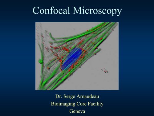
<strong>Confocal</strong> <strong>Microscopy</strong><br />
Dr. Serge Arnaudeau<br />
Bioimaging Core Facility<br />
Geneva
Light source<br />
Wide-field microscope<br />
in focus<br />
Sample<br />
(object plane)<br />
objective<br />
• only one plane in focus<br />
• but all the planes contribute to the image<br />
Viewing plane<br />
(image plane)
Light source<br />
in focus<br />
Sample<br />
(object plane)<br />
The pinhole<br />
objective<br />
Photons passing through the pinhole are coming<br />
exclusively from the focal point of the objective<br />
pinhole<br />
Viewing plane<br />
(image plane)
Depth of field depends on pinhole size<br />
in focus<br />
objective<br />
small pinhole<br />
large pinhole<br />
small pinhole most of the photons coming from out of<br />
focus planes are rejected and do not contribute to the image
Light<br />
source<br />
<strong>Confocal</strong> microscope principle<br />
pinhole<br />
Transmissive design<br />
• “conjugate focal planes”<br />
objective<br />
Sample<br />
(object plane)<br />
• illumination and detection of the same focal point<br />
• need to displace the sample in x and y to construct an image<br />
x<br />
y<br />
objective<br />
pinhole<br />
detector
Absorb high<br />
energy photons<br />
What is fluorescence?<br />
Excited state<br />
Emit lower<br />
energy photon<br />
Ground state<br />
In one-photon excitation λ ex < λ em (Stoke’s shift)
How does a fluorescence microscope<br />
Emission filter<br />
Dichroic filter<br />
objective<br />
work?<br />
Excitation filter<br />
sample<br />
Light source
Epitaxial confocal microscope for<br />
• use of the same objective for illumination<br />
and detection<br />
• use of a laser source to avoid the use of a<br />
pinhole in illumination<br />
fluorescence<br />
• use of a PMT to make photon counting for<br />
each focal point<br />
• use of galvanometric mirrors to XY scan the<br />
field of view<br />
• use of a stepping motor in the Z direction to<br />
make optical slices in the sample<br />
barrier filter<br />
photomultiplier tube<br />
pinhole<br />
dichroic mirror<br />
objective<br />
Focal point<br />
Laser Source
Advantage of fluorescence confocal<br />
• ability to control depth of field<br />
• elimination or reduction of<br />
background information away<br />
from the focal plane<br />
• capability to collect serial optical<br />
sections from thick specimens<br />
microscopy<br />
A section of mouse intestine<br />
imaged with both confocal and<br />
non-confocal microscopy
How big is a Laser Scanning <strong>Confocal</strong><br />
Laser module<br />
405, 458, 477, 488,<br />
514, 561, 633 nm<br />
System electronic rack<br />
Microscope ?<br />
Scanning head
LASER<br />
Light Amplification by Stimulated Emission of Radiation<br />
• High intensity<br />
• Spatial and temporal coherence<br />
• Monochromatic<br />
• Focused<br />
Lasers installed in our Laser Scanning Microscopes<br />
• 405 nm Diode laser (DAPI, CFP…)<br />
• Argon ion gas laser with 458 nm (CFP…)<br />
488 nm (FITC, GFP, Alexa 488 …)<br />
514 nm (YFP…)<br />
• Helium neon 543 nm gas laser (TRITC, Cy3, Alexa 546 …)<br />
• 561 nm DPSS laser (Texas red, Alexa 568 …)<br />
• Helium neon 633 nm gas laser (TOTO3, Cy5 …)
Wide-field illumination cone versus<br />
point scanning of specimens<br />
• Wide-field microscope : entire depth of the specimen over<br />
a wide area is illuminated<br />
• <strong>Confocal</strong> microscope : the sample is scanned with a finely<br />
focused spot of illumination centered in the focal plane
Beam scanning<br />
Majority of laser scanning microscopes : single beam<br />
scanning<br />
Laser spot<br />
To scan the specimen in a raster<br />
pattern, the Laser Scanning<br />
Microscope uses a pair of computer<br />
controlled galvanometric mirrors.<br />
The scanning speed is limited by<br />
these mirrors.<br />
Good image quality but not<br />
fast enough to resolve<br />
transient physiological signals<br />
Only confocal microscopes which use acousto-optic<br />
deflectors can scan at speeds of 30 frames/s
Photomultiplier Tubes (PMT)<br />
Photocathode<br />
Window<br />
Incident light<br />
Side on design<br />
Anode<br />
Dynodes<br />
Gain varies with the voltage across the dynodes and the total number of dynodes<br />
With typically 9 dynodes, gain of 4x10 6 can be achieved
Photomultiplier Tubes (PMT)<br />
The spectral response, quantum efficiency, sensitivity, and dark current of a<br />
photomultiplier tube are determined by the composition of the photocathode<br />
Quantum Efficiency (%)<br />
100<br />
10<br />
1<br />
0.1<br />
0.01<br />
100 200 300 400 500 600 700 800 900 1000<br />
Wavelength (nm)<br />
Gray levels (8bits)<br />
255<br />
128<br />
0<br />
600 V<br />
0 V<br />
800 V<br />
gain<br />
50 V offset<br />
Low quantum efficiency and low dynamic range but very fast response time
Scanning speed influences image<br />
quality<br />
pixel dwell time 3.2 µs pixel dwell time 25.6 µs<br />
Better signal to noise ratio with low scanning speeds but<br />
samples are more exposed to the laser beam<br />
2 µm<br />
Muntjac cells – Alexa 555 anti OX Phos complex V inh prot
Scans averaging reduces noise<br />
Average of 2 scans Average of 8 scans<br />
But greatly reduce the frame rate<br />
10 µm<br />
Muntjac cells – Alexa 488 phalloidin
Airy disk and Resolution<br />
Due to diffraction, the image of a point source of light in the focal<br />
plane is not a point it’s actually an Airy diffraction pattern<br />
Airy diffraction pattern<br />
Airy disk<br />
The resolving power of an objective determines the size of the<br />
Airy diffraction pattern formed
Airy disk and Resolution<br />
The radius of the Airy disk is given by :<br />
α<br />
r (Airy) = 0.61 λ exc /NA (obj)<br />
with NA (obj) = n sinα<br />
n = medium refractive index<br />
α = objective angular aperture
intensity<br />
Airy disk and Resolution<br />
Rayleigh criterion for lateral resolution :<br />
the center of one airy disk falls on the first minimum of the<br />
other airy disk<br />
contrast<br />
resolved Rayleigh criterion unresolved
Pinhole and Resolution<br />
<strong>Confocal</strong> pinhole size = diameter of the Airy disk (1 Airy unit)<br />
84% of in focus light pass to the detector<br />
Airy disk units are a convenient way to normalize confocal<br />
pinhole size :<br />
Pinhole size = 1 Airy unit = best signal to noise ratio
<strong>Confocal</strong> fluorescence :<br />
Pinhole and Resolution<br />
pointwise illumination + pointwise detection<br />
narrower Point Spread Function / widefield microscopy<br />
Axial PSF intensity profiles<br />
widefield confocal<br />
Increase in lateral resolution<br />
r lateral = 0.4 λ exc / NA<br />
confocal lateral resolution > widefield lateral resolution
Pinhole and Resolution<br />
<strong>Confocal</strong> PSF<br />
Axial resolution :<br />
r axial = 1.4 λ exc n/ NA 2<br />
The PSF is elongated in the axial direction<br />
Axial resolution of an objective is worse than<br />
its lateral resolution<br />
λ exc = excitation wavelength<br />
n = medium refractive index<br />
NA = objective’s numerical aperture<br />
For an oil immersion objective with 1.4 NA using the 488 nm laser line<br />
r lateral = 0.4 x 488/1.4 = 139 nm (in theory for very<br />
r axial = 1.4 x 488 x 1.515/(1.4) 2 = 528 nm small pinhole size)
Resolution depends on pinhole size<br />
Pinhole : 1 AU<br />
(optical slice ~ 0.8 µm)<br />
Pinhole : 0.5 AU<br />
(optical slice ~ 0.5 µm)<br />
Better Z discrimination with small pinhole size but needs<br />
strong signals<br />
10 µm<br />
Muntjac cells – Alexa 488 phalloidin
Z<br />
Optical sectionning<br />
Y<br />
X<br />
5<br />
4<br />
3<br />
2<br />
1<br />
z<br />
y<br />
x<br />
5<br />
4<br />
3<br />
2<br />
1<br />
3D reconstruction
Sampling in confocal microscopy<br />
Voxel on the sample<br />
z<br />
x<br />
y<br />
The image is built as the laser<br />
moves on the sample<br />
Zooming is produced by<br />
slower movement of the laser<br />
on a reduced area :<br />
no pixelization effect even<br />
with very high zoom<br />
y<br />
x<br />
Pixel on the image
Sampling in confocal microscopy<br />
260 nm/pixel<br />
16 nm/pixel<br />
512x512 zoom 1<br />
512x512 zoom 16<br />
20 µm<br />
1 µm<br />
130 nm/pixel<br />
33 nm/pixel<br />
512x512 zoom 2<br />
512x512 zoom 8<br />
10 µm<br />
2 µm<br />
65 nm/pixel<br />
512x512 zoom 4<br />
5 µm<br />
Muntjac cells<br />
Alexa 488 phalloidin<br />
Alexa 555 anti OXPhos complex V inh prot<br />
TO PRO-3
Sampling in confocal microscopy<br />
What is the zooming factor limit?<br />
This is linked to the X,Y resolution of the optics<br />
Sampling is sufficient when there is enough pixels to<br />
separate two adjacent Airy disk<br />
Nyquist theorem :<br />
to reconstruct a sine wave : f sampling = 2 x f wave<br />
In imaging, frequency = spatial frequency<br />
f sampling = 2.3 x f highest (to compensate low-pass filtering)
Sampling in confocal microscopy<br />
The highest frequency to be sampled in the CLSM is imposed<br />
by the optical system :<br />
f highest = 1/resolution<br />
To fulfill the Nyquist criterion :<br />
undersampling ><br />
f sampling = 2.3/r lateral<br />
Pixel size ~ r lateral /2.3 > oversampling
Sampling in confocal microscopy<br />
Critical sampling distances @ 500 nm<br />
(for pinhole = 1 AU values by 50%)
Ideal emission separation<br />
Red emission filter<br />
Dichroic<br />
beamsplitter<br />
λ τ<br />
PMT 1<br />
λ τ<br />
λ τ<br />
PMT 2<br />
Green emission filter
Crosstalk problems<br />
Most of the time there is some overlapping between<br />
fluorophores emission spectra<br />
Example of FITC and TRITC<br />
Using 488 nm and 543 nm lines : 22% overlap<br />
If the fluorescence signals<br />
are not taken sequentially :<br />
some of the green<br />
fluorescence is assigned to<br />
the red channel
Crosstalk problems<br />
To avoid bleed-through of one fluorescence in another<br />
channel, multitrack configurations allow sequential<br />
acquisition of lines (or frames) by very fast switching of the<br />
laser lines by means of AOTF<br />
Minimize crosstalk between channels<br />
More accurate quantification in co-localization experiments
Spectral separation<br />
When the emission spectra of the fluorophores are very close :<br />
Spectral detector (like the Meta detector) allow the record of the<br />
emission spectra of each pixel of the image<br />
Example of latex bead with<br />
narrow fluorescences in the<br />
core and the ring acquired<br />
with the spectral detector<br />
(Meta)<br />
Image serie of the bead at<br />
different wavelengths
Spectral separation<br />
Fluorescence separation<br />
after software unmixing<br />
Selection of the<br />
different fluorescences<br />
(core and ring)
FRAP<br />
Fluorescence Recovery After Photobleaching<br />
bleach recovery<br />
Use of the high power of the laser to photobleach<br />
a defined region of the sample<br />
The recovery of fluorescence in this region indicates<br />
any kind of movement (diffusion or transport) of<br />
fluorescent molecules<br />
The recovery time (half-recovery time) indicates the<br />
speed of this mobility
FRAP experiments<br />
FRAP-recording for 40 min (1 frame/min)
Very high control of the scanner<br />
by the DSP (Digital Signal<br />
Processor) to position the laser<br />
beam and choose ROI of any<br />
shape<br />
Photobleaching<br />
Bovine endothelial cells<br />
actin filaments (BODIPY FL),<br />
mitochondria (MitoTracker Red);<br />
some mitochondria are marked<br />
for photobleaching<br />
Bleaching of marked mitochondria with pinpoint<br />
accuracy (left)<br />
Merged images of mitochondria before and after<br />
photobleaching :bleached portions appeared in red<br />
(right)
Other beam scanning techniques<br />
Multiple beam scanning : the Nipkow disk<br />
Disk rotation<br />
One way to increase the scanning<br />
speed is to increase the number<br />
of scanning spots.<br />
The spinning disk with pinholes<br />
was introduced into a microscope<br />
by Mojmir Petran in 1968.
Improvement of the Nipkow disk<br />
principle in the YOKOGAWA scanhead<br />
Collector disk<br />
Aperture disk<br />
Objective<br />
specimen<br />
Dichroic<br />
mirror<br />
Laser beam<br />
Microlenses<br />
(20 000)<br />
Pinholes<br />
(20 000)<br />
CCD camera
Nipkow disk confocal microscope facilitate<br />
Cell cycle in<br />
Drosophila Embryo<br />
expressing GFP-<br />
Histone<br />
Dr. Caetano Gonzalez<br />
EMBL<br />
studies of ligth-sensitive processes
Nipkow disk confocal microscope facilitate<br />
Ca 2+ waves in<br />
cardiomyocytes<br />
loaded with fluo-3<br />
Dr. Marisa Jaconi<br />
Geneva<br />
studies of fast processes<br />
Image capture at 33 Hz using an intensified camera<br />
(Coolsnap Cascade from Photometrics)
Other beam scanning techniques<br />
Slit scanning : a new approach in confocal microscopy<br />
•The circular laser beam is transformed<br />
to a line which scan the sample in only<br />
one direction<br />
•The emitted fluorescence of that line<br />
passed through a confocal line pinhole<br />
•This line (512 pixels) is detected by a<br />
ultrafast line CCD detector<br />
Scan speeds of 100 frames/s<br />
can be achieved
Fluo-3<br />
Fura-red<br />
10 μm<br />
Advantage of the LSCM :<br />
the line scan mode<br />
10 μm<br />
[Ca 2+ ] i (nM)<br />
150<br />
75<br />
0<br />
200 ms<br />
Spatially restricted, but very fast (1 line/2ms)<br />
250<br />
125<br />
0<br />
[Ca 2+ ] i (nM)