Bornhuetter--Ferguson as a General Principle of Loss Reserving
Bornhuetter--Ferguson as a General Principle of Loss Reserving
Bornhuetter--Ferguson as a General Principle of Loss Reserving

You also want an ePaper? Increase the reach of your titles
YUMPU automatically turns print PDFs into web optimized ePapers that Google loves.
ROT DP oBF eBF SC BFP Ex Ref<br />
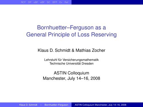
<strong>Bornhuetter</strong>–<strong>Ferguson</strong> <strong>as</strong> a<br />
<strong>General</strong> <strong>Principle</strong> <strong>of</strong> <strong>Loss</strong> <strong>Reserving</strong><br />
Klaus D. Schmidt & Mathi<strong>as</strong> Zocher<br />
Lehrstuhl für Versicherungsmathematik<br />
Technische Universität Dresden<br />
ASTIN Colloquium<br />
Manchester, July 14–16, 2008<br />
Klaus D. Schmidt – <strong>Bornhuetter</strong>–<strong>Ferguson</strong> ASTIN Colloquium Manchester, July 14–16, 2008
ROT DP oBF eBF SC BFP Ex Ref<br />
Table <strong>of</strong> Contents<br />
Run–Off Triangles <strong>of</strong> Cumulative <strong>Loss</strong>es<br />
Development Patterns<br />
The original <strong>Bornhuetter</strong>–<strong>Ferguson</strong> Method<br />
The extended <strong>Bornhuetter</strong>–<strong>Ferguson</strong> Method<br />
Special C<strong>as</strong>es<br />
The <strong>Loss</strong>–Development Method<br />
The Chain–Ladder Method<br />
The Cape Cod Method<br />
The Additive Method<br />
The <strong>Bornhuetter</strong>–<strong>Ferguson</strong> <strong>Principle</strong><br />
An Example<br />
References<br />
Klaus D. Schmidt – <strong>Bornhuetter</strong>–<strong>Ferguson</strong> ASTIN Colloquium Manchester, July 14–16, 2008
ROT DP oBF eBF SC BFP Ex Ref<br />
Run–Off Triangles <strong>of</strong> Cumulative <strong>Loss</strong>es (1)<br />
An example from the Claims <strong>Reserving</strong> Manual:<br />
Accident Development Year<br />
Year 0 1 2 3 4 5<br />
0 1001 1855 2423 2988 3335 3483<br />
1 1113 2103 2774 3422 3844<br />
2 1265 2433 3233 3977<br />
3 1490 2873 3880<br />
4 1725 3261<br />
5 1889<br />
The enumeration <strong>of</strong> the development years represents delays<br />
with respect to the accident years.<br />
Klaus D. Schmidt – <strong>Bornhuetter</strong>–<strong>Ferguson</strong> ASTIN Colloquium Manchester, July 14–16, 2008
ROT DP oBF eBF SC BFP Ex Ref<br />
Run–Off Triangles <strong>of</strong> Cumulative <strong>Loss</strong>es (2)<br />
Accident Development Year<br />
Year 0 1 . . . k . . . n − i . . . n − 1 n<br />
0 S 0,0 S 0,1 . . . S 0,k . . . S 0,n−i . . . S 0,n−1 S 0,n<br />
1 S 1,0 S 1,1 . . . S 1,k . . . S 1,n−i . . . S 1,n−1 S 1,n<br />
.<br />
.<br />
.<br />
.<br />
i S i,0 S i,1 . . . S i,k . . . S i,n−i . . . S i,n−1 S i,n<br />
.<br />
.<br />
.<br />
.<br />
n−k S n−k,0 S n−k,1 . . . S n−k,k . . . S n−k,n−i . . . S n−k,n−1 S n−k,n<br />
.<br />
.<br />
.<br />
.<br />
n−1 S n−1,0 S n−1,1 . . . S n−1,k . . . S n−1,n−i . . . S n−1,n−1 S n−1,n<br />
n S n,0 S n,1 . . . S n,k . . . S n,n−i . . . S n,n−1 Sn,n<br />
A cumulative loss Si,k is said to be<br />
◮ observable if i + k ≤ n.<br />
◮ non–observable or future if i + k > n.<br />
◮ current if i + k = n.<br />
◮ ultimate if k = n.<br />
Klaus D. Schmidt – <strong>Bornhuetter</strong>–<strong>Ferguson</strong> ASTIN Colloquium Manchester, July 14–16, 2008<br />
.<br />
.<br />
.<br />
.<br />
.<br />
.<br />
.<br />
.<br />
.
ROT DP oBF eBF SC BFP Ex Ref<br />
Run–Off Triangles <strong>of</strong> Cumulative <strong>Loss</strong>es (3)<br />
The purpose <strong>of</strong> loss reserving is to predict<br />
◮ the ultimate losses Si,n and<br />
◮ the accident year reserves Si,n − Si,n−i<br />
More generally: The aim is to predict<br />
◮ the future cumulative losses Si,k<br />
◮ the future incremental losses Zi,k := Si,k − Si,k−1<br />
◮ the calendar year reserves n<br />
◮ the total reserve n<br />
j=1<br />
j=p−n Zj,p−j<br />
n<br />
l=n−j+1 Zj,l<br />
with i + k ≥ n + 1 and p = n + 1, . . . , 2n.<br />
Thus: The principal t<strong>as</strong>k considered here is to predict the future<br />
cumulative losses.<br />
Klaus D. Schmidt – <strong>Bornhuetter</strong>–<strong>Ferguson</strong> ASTIN Colloquium Manchester, July 14–16, 2008
ROT DP oBF eBF SC BFP Ex Ref<br />
Table <strong>of</strong> Contents<br />
Run–Off Triangles <strong>of</strong> Cumulative <strong>Loss</strong>es<br />
Development Patterns<br />
The original <strong>Bornhuetter</strong>–<strong>Ferguson</strong> Method<br />
The extended <strong>Bornhuetter</strong>–<strong>Ferguson</strong> Method<br />
Special C<strong>as</strong>es<br />
The <strong>Loss</strong>–Development Method<br />
The Chain–Ladder Method<br />
The Cape Cod Method<br />
The Additive Method<br />
The <strong>Bornhuetter</strong>–<strong>Ferguson</strong> <strong>Principle</strong><br />
An Example<br />
References<br />
Klaus D. Schmidt – <strong>Bornhuetter</strong>–<strong>Ferguson</strong> ASTIN Colloquium Manchester, July 14–16, 2008
ROT DP oBF eBF SC BFP Ex Ref<br />
Development Patterns<br />
◮ A development pattern for quot<strong>as</strong> consists <strong>of</strong> parameters<br />
γ0, γ1, . . . , γn with<br />
γk = E[Si,k]/E[Si,n]<br />
for all k = 0, 1, . . . , n and for all i = 0, 1, . . . , n.<br />
These parameters are called development quot<strong>as</strong><br />
(percentages reported).<br />
◮ A development pattern for factors consists <strong>of</strong> parameters<br />
ϕ1, . . . , ϕn with<br />
ϕk = E[Si,k]/E[Si,k−1]<br />
for all k = 1, . . . , n and for all i = 0, 1, . . . , n.<br />
These parameters are called development factors<br />
(age–to–age factors).<br />
Klaus D. Schmidt – <strong>Bornhuetter</strong>–<strong>Ferguson</strong> ASTIN Colloquium Manchester, July 14–16, 2008
ROT DP oBF eBF SC BFP Ex Ref<br />
Development Patterns:<br />
Cumulative <strong>Loss</strong>es and Quot<strong>as</strong><br />
Accident Development Year<br />
Year 0 1 2 3 4 5<br />
0 1001 1855 2423 2988 3335 3483<br />
1 1113 2103 2774 3422 3844 4044<br />
2 1265 2433 3233 3977 4477 4677<br />
3 1490 2873 3880 4880 5380 5680<br />
4 1725 3261 4361 5461 5961 6361<br />
5 1889 3489 4889 5889 6489 6889<br />
0 0.287 0.533 0.696 0.858 0.958 1.000<br />
1 0.275 0.520 0.686 0.846 0.951 1.000<br />
2 0.270 0.520 0.691 0.850 0.957 1.000<br />
3 0.262 0.506 0.683 0.859 0.947 1.000<br />
4 0.271 0.513 0.686 0.859 0.937 1.000<br />
5 0.274 0.506 0.710 0.855 0.942 1.000<br />
Klaus D. Schmidt – <strong>Bornhuetter</strong>–<strong>Ferguson</strong> ASTIN Colloquium Manchester, July 14–16, 2008
ROT DP oBF eBF SC BFP Ex Ref<br />
Development Patterns:<br />
Cumulative <strong>Loss</strong>es and Factors<br />
Accident Development Year<br />
Year 0 1 2 3 4 5<br />
0 1001 1855 2423 2988 3335 3483<br />
1 1113 2103 2774 3422 3844 4044<br />
2 1265 2433 3233 3977 4477 4677<br />
3 1490 2873 3880 4880 5380 5680<br />
4 1725 3261 4361 5461 5961 6361<br />
5 1889 3489 4889 5889 6489 6889<br />
0 1.853 1.306 1.233 1.116 1.044<br />
1 1.889 1.319 1.234 1.123 1.052<br />
2 1.923 1.329 1.230 1.126 1.045<br />
3 1.928 1.351 1.258 1.102 1.056<br />
4 1.890 1.337 1.252 1.092 1.067<br />
5 1.847 1.401 1.205 1.102 1.062<br />
Klaus D. Schmidt – <strong>Bornhuetter</strong>–<strong>Ferguson</strong> ASTIN Colloquium Manchester, July 14–16, 2008
ROT DP oBF eBF SC BFP Ex Ref<br />
Development Patterns: Quot<strong>as</strong> and Factors<br />
◮ If the parameters γ0, γ1, . . . , γn form a development pattern<br />
for quot<strong>as</strong>, then the parameters ϕ1, . . . , ϕn with<br />
ϕk := γk<br />
γk−1<br />
form a development pattern for factors.<br />
◮ If the parameters ϕ1, . . . , ϕn form a development pattern<br />
for factors, then the parameters γ0, γ1, . . . , γn with<br />
γk :=<br />
n<br />
1<br />
ϕl<br />
l=k+1<br />
form a development pattern for quot<strong>as</strong>.<br />
Klaus D. Schmidt – <strong>Bornhuetter</strong>–<strong>Ferguson</strong> ASTIN Colloquium Manchester, July 14–16, 2008
ROT DP oBF eBF SC BFP Ex Ref<br />
Development Patterns: Estimation <strong>of</strong> Quot<strong>as</strong><br />
For estimation <strong>of</strong> the parameter γk <strong>of</strong> a development pattern for<br />
quot<strong>as</strong>, the only obvious estimator provided by the run–<strong>of</strong>f<br />
triangle is the empirical individual quota<br />
γ0,k := S0,k/S0,n<br />
Accident Development Year<br />
Year 0 1 2 3 4 5<br />
0 0.287 0.533 0.696 0.858 0.958 1.000<br />
1 0.275 0.520 0.686 0.846 0.951 1.000<br />
2 0.270 0.520 0.691 0.850 0.957 1.000<br />
3 0.262 0.506 0.683 0.859 0.947 1.000<br />
4 0.271 0.513 0.686 0.859 0.937 1.000<br />
5 0.274 0.506 0.710 0.855 0.942 1.000<br />
Klaus D. Schmidt – <strong>Bornhuetter</strong>–<strong>Ferguson</strong> ASTIN Colloquium Manchester, July 14–16, 2008
ROT DP oBF eBF SC BFP Ex Ref<br />
Development Patterns: Estimation <strong>of</strong> Factors<br />
For estimation <strong>of</strong> the parameter ϕk <strong>of</strong> a development pattern for<br />
factors, the run–<strong>of</strong>f triangle provides the empirical individual<br />
factors<br />
ϕi,k := Si,k/Si,k−1<br />
with i = 0, 1, . . . , n − k. Moreover, any weighted mean <strong>of</strong> these<br />
estimators is an estimator <strong>as</strong> well.<br />
Accident Development Year<br />
Year 0 1 2 3 4 5<br />
0 1.853 1.306 1.233 1.116 1.044<br />
1 1.889 1.319 1.234 1.123 1.052<br />
2 1.923 1.329 1.230 1.126 1.045<br />
3 1.928 1.351 1.258 1.102 1.056<br />
4 1.890 1.337 1.252 1.092 1.067<br />
5 1.847 1.401 1.205 1.102 1.062<br />
Klaus D. Schmidt – <strong>Bornhuetter</strong>–<strong>Ferguson</strong> ASTIN Colloquium Manchester, July 14–16, 2008
ROT DP oBF eBF SC BFP Ex Ref<br />
Development Patterns: Chain–Ladder Factors<br />
The chain–ladder factors<br />
ϕ CL<br />
k :=<br />
n−k<br />
j=0 Sj,k<br />
n−k<br />
j=0 Sj,k−1<br />
=<br />
n−k Sj,k−1<br />
n−k j=0 h=0 Sh,k−1<br />
ϕj,k<br />
are weighted means and may be used to estimate the<br />
development factors ϕk.<br />
Accident Development Year k<br />
Year i 0 1 2 3 4 5<br />
0 1001 1855 2423 2988 3335 3483<br />
1 1113 2103 2774 3422 3844<br />
2 1265 2433 3233 3977<br />
3 1490 2873 3880<br />
4 1725 3261<br />
5 1889<br />
bϕ CL<br />
k 1.899 1.329 1.232 1.120 1.044<br />
Klaus D. Schmidt – <strong>Bornhuetter</strong>–<strong>Ferguson</strong> ASTIN Colloquium Manchester, July 14–16, 2008
ROT DP oBF eBF SC BFP Ex Ref<br />
Development Patterns: Chain–Ladder Quot<strong>as</strong><br />
The chain–ladder quot<strong>as</strong><br />
γ CL<br />
k :=<br />
n<br />
l=k+1<br />
1<br />
ϕ CL<br />
l<br />
may be used to estimate the development quot<strong>as</strong> γk.<br />
Accident Development Year k<br />
Year i 0 1 2 3 4 5<br />
0 1001 1855 2423 2988 3335 3483<br />
1 1113 2103 2774 3422 3844<br />
2 1265 2433 3233 3977<br />
3 1490 2873 3880<br />
4 1725 3261<br />
5 1889<br />
bϕ CL<br />
k 1.899 1.329 1.232 1.120 1.044<br />
bγ CL<br />
k 0.278 0.527 0.701 0.864 0.968 1<br />
Klaus D. Schmidt – <strong>Bornhuetter</strong>–<strong>Ferguson</strong> ASTIN Colloquium Manchester, July 14–16, 2008
ROT DP oBF eBF SC BFP Ex Ref<br />
Table <strong>of</strong> Contents<br />
Run–Off Triangles <strong>of</strong> Cumulative <strong>Loss</strong>es<br />
Development Patterns<br />
The original <strong>Bornhuetter</strong>–<strong>Ferguson</strong> Method<br />
The extended <strong>Bornhuetter</strong>–<strong>Ferguson</strong> Method<br />
Special C<strong>as</strong>es<br />
The <strong>Loss</strong>–Development Method<br />
The Chain–Ladder Method<br />
The Cape Cod Method<br />
The Additive Method<br />
The <strong>Bornhuetter</strong>–<strong>Ferguson</strong> <strong>Principle</strong><br />
An Example<br />
References<br />
Klaus D. Schmidt – <strong>Bornhuetter</strong>–<strong>Ferguson</strong> ASTIN Colloquium Manchester, July 14–16, 2008
ROT DP oBF eBF SC BFP Ex Ref<br />
The original <strong>Bornhuetter</strong>–<strong>Ferguson</strong> Method (1)<br />
In its original version, the <strong>Bornhuetter</strong>–<strong>Ferguson</strong> method aims<br />
at predicting calendar year reserves<br />
Ri := Si,n − Si,n−i<br />
If γ0, γ1, . . . , γn is a development pattern for quot<strong>as</strong>, then the<br />
expected reserves satisfy the model equation<br />
<br />
E[Ri] = 1 − γn−i E[Si,n]<br />
The original <strong>Bornhuetter</strong>–<strong>Ferguson</strong> predictors <strong>of</strong> the reserves<br />
Ri are defined <strong>as</strong><br />
<br />
Ri := 1 − γ CL<br />
<br />
n−i πi κi<br />
where<br />
◮ γ CL<br />
n−i<br />
is the current chain–ladder quota,<br />
◮ πi is a volume me<strong>as</strong>ure, and<br />
◮ κi is an estimator <strong>of</strong> the expected loss ratio κi := E[Si,n/πi]<br />
Klaus D. Schmidt – <strong>Bornhuetter</strong>–<strong>Ferguson</strong> ASTIN Colloquium Manchester, July 14–16, 2008
ROT DP oBF eBF SC BFP Ex Ref<br />
The original <strong>Bornhuetter</strong>–<strong>Ferguson</strong> Method (2)<br />
◮ Transformation into predictors <strong>of</strong> the ultimate losses Si,n:<br />
Si,n := Si,n−i +<br />
<br />
1 − γ CL<br />
<br />
n−i πi κi<br />
◮ Transformation into predictors <strong>of</strong> other future cumulative<br />
losses Si,k:<br />
<br />
Si,k := Si,n−i + γ CL<br />
<br />
k − γCL n−i πi κi<br />
Idea:<br />
◮ Replace the chain–ladder quot<strong>as</strong> by arbitrary estimators <strong>of</strong><br />
the quot<strong>as</strong>.<br />
◮ Replace the estimators πi κi by arbitrary estimators <strong>of</strong> the<br />
expected ultimate losses E[Si,n].<br />
Klaus D. Schmidt – <strong>Bornhuetter</strong>–<strong>Ferguson</strong> ASTIN Colloquium Manchester, July 14–16, 2008
ROT DP oBF eBF SC BFP Ex Ref<br />
Table <strong>of</strong> Contents<br />
Run–Off Triangles <strong>of</strong> Cumulative <strong>Loss</strong>es<br />
Development Patterns<br />
The original <strong>Bornhuetter</strong>–<strong>Ferguson</strong> Method<br />
The extended <strong>Bornhuetter</strong>–<strong>Ferguson</strong> Method<br />
Special C<strong>as</strong>es<br />
The <strong>Loss</strong>–Development Method<br />
The Chain–Ladder Method<br />
The Cape Cod Method<br />
The Additive Method<br />
The <strong>Bornhuetter</strong>–<strong>Ferguson</strong> <strong>Principle</strong><br />
An Example<br />
References<br />
Klaus D. Schmidt – <strong>Bornhuetter</strong>–<strong>Ferguson</strong> ASTIN Colloquium Manchester, July 14–16, 2008
ROT DP oBF eBF SC BFP Ex Ref<br />
The extended <strong>Bornhuetter</strong>–<strong>Ferguson</strong> Method (1)<br />
The extended <strong>Bornhuetter</strong>–<strong>Ferguson</strong> method is b<strong>as</strong>ed on the<br />
<strong>as</strong>sumption, that there exists a development pattern for quot<strong>as</strong><br />
and that<br />
◮ prior estimators<br />
γ0, γ1, . . . , γn<br />
(with γn = 1) <strong>of</strong> the development quot<strong>as</strong> γ0, γ1, . . . , γn and<br />
◮ prior estimators<br />
α0, α1, . . . , αn<br />
<strong>of</strong> the expected ultimate losses<br />
with i = 0, 1, . . . , n<br />
are available.<br />
αi := E[Si,n]<br />
Klaus D. Schmidt – <strong>Bornhuetter</strong>–<strong>Ferguson</strong> ASTIN Colloquium Manchester, July 14–16, 2008
ROT DP oBF eBF SC BFP Ex Ref<br />
The extended <strong>Bornhuetter</strong>–<strong>Ferguson</strong> Method (2)<br />
These prior estimators can be obtained from<br />
◮ internal information (provided by the run–<strong>of</strong>f triangle, like<br />
chain–ladder factors),<br />
◮ volume me<strong>as</strong>ures (like premiums) for the portfolio under<br />
consideration,<br />
◮ external information (market statistics or data from similar<br />
portfolios) or<br />
◮ a combination <strong>of</strong> these data.<br />
Klaus D. Schmidt – <strong>Bornhuetter</strong>–<strong>Ferguson</strong> ASTIN Colloquium Manchester, July 14–16, 2008
ROT DP oBF eBF SC BFP Ex Ref<br />
The extended <strong>Bornhuetter</strong>–<strong>Ferguson</strong> Method (3)<br />
The future cumulative losses satisfy the model equation<br />
E[Si,k] = E[Si,n−i] +<br />
<br />
γk − γn−i<br />
<br />
E[Si,n]<br />
Accordingly, the extended <strong>Bornhuetter</strong>–<strong>Ferguson</strong> predictors <strong>of</strong><br />
the future cumulative losses are defined <strong>as</strong><br />
S BF<br />
i,k := Si,n−i<br />
<br />
+ γk − γn−i αi<br />
Thus:<br />
◮ The run–<strong>of</strong>f triangle provides information perhaps only via<br />
the current losses.<br />
◮ The predictors <strong>of</strong> the ultimate losses are obtained by linear<br />
extrapolation from the current losses.<br />
Klaus D. Schmidt – <strong>Bornhuetter</strong>–<strong>Ferguson</strong> ASTIN Colloquium Manchester, July 14–16, 2008
ROT DP oBF eBF SC BFP Ex Ref<br />
The extended <strong>Bornhuetter</strong>–<strong>Ferguson</strong> Method (4)<br />
Accident Development Year k<br />
Year i 0 1 2 3 4 5 bαi<br />
0 3483 3517<br />
1 3844 4043 3981<br />
2 3977 4391 4621 4598<br />
3 3880 4785 4389 5577 5658<br />
4 3261 4442 5436 5995 6306 6214<br />
5 1889 3344 4546 5558 6127 6443 6325<br />
bγk 0.280 0.510 0.700 0.860 0.950 1.000<br />
1 − bγk 0.720 0.490 0.300 0.140 0.050 0.000<br />
Klaus D. Schmidt – <strong>Bornhuetter</strong>–<strong>Ferguson</strong> ASTIN Colloquium Manchester, July 14–16, 2008
ROT DP oBF eBF SC BFP Ex Ref LD CL CC AD<br />
Table <strong>of</strong> Contents<br />
Run–Off Triangles <strong>of</strong> Cumulative <strong>Loss</strong>es<br />
Development Patterns<br />
The original <strong>Bornhuetter</strong>–<strong>Ferguson</strong> Method<br />
The extended <strong>Bornhuetter</strong>–<strong>Ferguson</strong> Method<br />
Special C<strong>as</strong>es<br />
The <strong>Loss</strong>–Development Method<br />
The Chain–Ladder Method<br />
The Cape Cod Method<br />
The Additive Method<br />
The <strong>Bornhuetter</strong>–<strong>Ferguson</strong> <strong>Principle</strong><br />
An Example<br />
References<br />
Klaus D. Schmidt – <strong>Bornhuetter</strong>–<strong>Ferguson</strong> ASTIN Colloquium Manchester, July 14–16, 2008
ROT DP oBF eBF SC BFP Ex Ref LD CL CC AD<br />
The <strong>Loss</strong>–Development Method (1)<br />
The loss–development method is b<strong>as</strong>ed on the <strong>as</strong>sumption,<br />
that there exists a development pattern for quot<strong>as</strong> and that prior<br />
estimators<br />
γ0, γ1, . . . , γn<br />
(with γn = 1) <strong>of</strong> the development quot<strong>as</strong> γ0, γ1, . . . , γn are<br />
available.<br />
The loss–development method does not involve any prior<br />
estimators for the expected ultimate losses.<br />
Klaus D. Schmidt – <strong>Bornhuetter</strong>–<strong>Ferguson</strong> ASTIN Colloquium Manchester, July 14–16, 2008
ROT DP oBF eBF SC BFP Ex Ref LD CL CC AD<br />
The <strong>Loss</strong>–Development Method (2)<br />
The future cumulative losses satisfy the model equation<br />
E[Si,n−i]<br />
E[Si,k] = γk<br />
γn−i<br />
Accordingly, the loss–development predictors <strong>of</strong> the future<br />
cumulative losses are defined <strong>as</strong><br />
Thus:<br />
S LD<br />
i,k<br />
:= γk<br />
Si,n−i<br />
γn−i<br />
◮ The run–<strong>of</strong>f triangle provides information perhaps only via<br />
the current losses.<br />
◮ The predictors <strong>of</strong> the ultimate losses are obtained by<br />
scaling the current losses.<br />
◮ The predictors <strong>of</strong> other future cumulative losses are<br />
obtained by scaling the predictors <strong>of</strong> the ultimate losses.<br />
Klaus D. Schmidt – <strong>Bornhuetter</strong>–<strong>Ferguson</strong> ASTIN Colloquium Manchester, July 14–16, 2008
ROT DP oBF eBF SC BFP Ex Ref LD CL CC AD<br />
The <strong>Loss</strong>–Development Method (3)<br />
Accident Development Year k<br />
Year i 0 1 2 3 4 5<br />
0 3483<br />
1 3844 4046<br />
2 3977 4393 4624<br />
3 3880 4767 5266 5543<br />
4 3261 4476 5499 6074 6394<br />
5 1889 3440 4722 5802 6409 6746<br />
bγk 0,280 0,510 0,700 0,860 0,950 1,000<br />
Klaus D. Schmidt – <strong>Bornhuetter</strong>–<strong>Ferguson</strong> ASTIN Colloquium Manchester, July 14–16, 2008
ROT DP oBF eBF SC BFP Ex Ref LD CL CC AD<br />
The <strong>Loss</strong>–Development Method (4)<br />
Because <strong>of</strong> the definition<br />
S LD<br />
i,k<br />
:= γk<br />
Si,n−i<br />
γn−i<br />
the loss–development predictors can be written <strong>as</strong><br />
S LD<br />
i,k = Si,n−i<br />
<br />
Si,n−i<br />
+ γk − γn−i<br />
γn−i<br />
In this form, the loss–development predictors attain the shape<br />
<strong>of</strong> the extended <strong>Bornhuetter</strong>–<strong>Ferguson</strong> predictors with respect<br />
to the prior estimators<br />
α LD<br />
i<br />
<strong>of</strong> the expected ultimate losses.<br />
:= Si,n−i<br />
γn−i<br />
Klaus D. Schmidt – <strong>Bornhuetter</strong>–<strong>Ferguson</strong> ASTIN Colloquium Manchester, July 14–16, 2008
ROT DP oBF eBF SC BFP Ex Ref LD CL CC AD<br />
Table <strong>of</strong> Contents<br />
Run–Off Triangles <strong>of</strong> Cumulative <strong>Loss</strong>es<br />
Development Patterns<br />
The original <strong>Bornhuetter</strong>–<strong>Ferguson</strong> Method<br />
The extended <strong>Bornhuetter</strong>–<strong>Ferguson</strong> Method<br />
Special C<strong>as</strong>es<br />
The <strong>Loss</strong>–Development Method<br />
The Chain–Ladder Method<br />
The Cape Cod Method<br />
The Additive Method<br />
The <strong>Bornhuetter</strong>–<strong>Ferguson</strong> <strong>Principle</strong><br />
An Example<br />
References<br />
Klaus D. Schmidt – <strong>Bornhuetter</strong>–<strong>Ferguson</strong> ASTIN Colloquium Manchester, July 14–16, 2008
ROT DP oBF eBF SC BFP Ex Ref LD CL CC AD<br />
The Chain–Ladder Method (1)<br />
The chain–ladder method is b<strong>as</strong>ed on the <strong>as</strong>sumption that<br />
there exists a development pattern for factors.<br />
The chain–ladder method relies completely on the observable<br />
cumulative losses <strong>of</strong> the run–<strong>of</strong>f triangle and involves no prior<br />
estimators at all.<br />
As estimators <strong>of</strong> the development factors, the chain–ladder<br />
method uses the chain–ladder factors<br />
ϕ CL<br />
n−k j=0<br />
k :=<br />
Sj,k<br />
n−k j=0 Sj,k−1<br />
n−k Sj,k−1<br />
= n−k h=0 Sh,k−1<br />
ϕj,k<br />
Klaus D. Schmidt – <strong>Bornhuetter</strong>–<strong>Ferguson</strong> ASTIN Colloquium Manchester, July 14–16, 2008<br />
j=0
ROT DP oBF eBF SC BFP Ex Ref LD CL CC AD<br />
The Chain–Ladder Method (2)<br />
The future cumulative losses Si,k satisfy the model equation<br />
E[Si,k] = E[Si,n−i]<br />
k<br />
l=n−i+1<br />
Accordingly, the chain–ladder predictors <strong>of</strong> the future<br />
cumulative losses are defined <strong>as</strong><br />
Thus:<br />
S CL<br />
i,k<br />
k<br />
:= Si,n−i<br />
l=n−i+1<br />
ϕ CL<br />
l<br />
◮ The chain–ladder method consists in successive scaling <strong>of</strong><br />
the current loss Si,n−i to the level <strong>of</strong> the future cumulative<br />
loss Si,k.<br />
Klaus D. Schmidt – <strong>Bornhuetter</strong>–<strong>Ferguson</strong> ASTIN Colloquium Manchester, July 14–16, 2008<br />
ϕl
ROT DP oBF eBF SC BFP Ex Ref LD CL CC AD<br />
The Chain–Ladder Method (3)<br />
Accident Development Year k<br />
Year i 0 1 2 3 4 5<br />
0 1001 1855 2423 2988 3335 3483<br />
1 1113 2103 2774 3422 3844 4013<br />
2 1265 2433 3233 3977 4454 4650<br />
3 1490 2873 3880 4780 5354 5590<br />
4 1725 3261 4334 5339 5980 6243<br />
5 1889 3587 4767 5873 6578 6867<br />
bϕ CL<br />
k 1,899 1,329 1,232 1,120 1,044<br />
Klaus D. Schmidt – <strong>Bornhuetter</strong>–<strong>Ferguson</strong> ASTIN Colloquium Manchester, July 14–16, 2008
ROT DP oBF eBF SC BFP Ex Ref LD CL CC AD<br />
The Chain–Ladder Method (4)<br />
Because <strong>of</strong> the definition<br />
S CL<br />
i,k<br />
k<br />
:= Si,n−i<br />
l=n−i+1<br />
ϕ CL<br />
l<br />
the chain–ladder predictors <strong>of</strong> the future cumulative losses can<br />
be written <strong>as</strong><br />
S CL<br />
i,k<br />
= γCL<br />
k<br />
Si,n−i<br />
γ CL<br />
n−i<br />
In this form, the chain–ladder predictors attain the shape <strong>of</strong> the<br />
loss–development predictors with respect to the chain–ladder<br />
quot<strong>as</strong>.<br />
Klaus D. Schmidt – <strong>Bornhuetter</strong>–<strong>Ferguson</strong> ASTIN Colloquium Manchester, July 14–16, 2008
ROT DP oBF eBF SC BFP Ex Ref LD CL CC AD<br />
The Chain–Ladder Method (5)<br />
Since<br />
S CL<br />
i,k<br />
= γCL<br />
k<br />
Si,n−i<br />
γ CL<br />
n−i<br />
the chain–ladder predictors <strong>of</strong> the future cumulative losses can<br />
also be written <strong>as</strong><br />
S CL<br />
i,k = Si,n−i<br />
<br />
+ γ CL<br />
<br />
Si,n−i<br />
k − γCL n−i<br />
γ CL<br />
n−i<br />
In this form, the chain–ladder predictors attain the shape <strong>of</strong> the<br />
extended <strong>Bornhuetter</strong>–<strong>Ferguson</strong> predictors with respect to the<br />
chain–ladder quot<strong>as</strong> and the prior estimators<br />
α CL<br />
i<br />
<strong>of</strong> the expected ultimate losses.<br />
:= Si,n−i<br />
γ CL<br />
n−i<br />
Klaus D. Schmidt – <strong>Bornhuetter</strong>–<strong>Ferguson</strong> ASTIN Colloquium Manchester, July 14–16, 2008
ROT DP oBF eBF SC BFP Ex Ref LD CL CC AD<br />
Table <strong>of</strong> Contents<br />
Run–Off Triangles <strong>of</strong> Cumulative <strong>Loss</strong>es<br />
Development Patterns<br />
The original <strong>Bornhuetter</strong>–<strong>Ferguson</strong> Method<br />
The extended <strong>Bornhuetter</strong>–<strong>Ferguson</strong> Method<br />
Special C<strong>as</strong>es<br />
The <strong>Loss</strong>–Development Method<br />
The Chain–Ladder Method<br />
The Cape Cod Method<br />
The Additive Method<br />
The <strong>Bornhuetter</strong>–<strong>Ferguson</strong> <strong>Principle</strong><br />
An Example<br />
References<br />
Klaus D. Schmidt – <strong>Bornhuetter</strong>–<strong>Ferguson</strong> ASTIN Colloquium Manchester, July 14–16, 2008
ROT DP oBF eBF SC BFP Ex Ref LD CL CC AD<br />
The Cape Cod Method (1)<br />
The Cape Cod method is b<strong>as</strong>ed on the <strong>as</strong>sumption, that there<br />
exists a development pattern for quot<strong>as</strong> and that prior<br />
estimators<br />
γ0, γ1, . . . , γn<br />
(with γn = 1) <strong>of</strong> the development quot<strong>as</strong> γ0, γ1, . . . , γn are<br />
available.<br />
It is also b<strong>as</strong>ed on the <strong>as</strong>sumption that there exist volume<br />
me<strong>as</strong>ures π0, π1, . . . , πn for the accident years and that the<br />
expected ultimate loss ratio<br />
<br />
Si,n<br />
κ := E<br />
is the same for all accident years.<br />
Klaus D. Schmidt – <strong>Bornhuetter</strong>–<strong>Ferguson</strong> ASTIN Colloquium Manchester, July 14–16, 2008<br />
πi
ROT DP oBF eBF SC BFP Ex Ref LD CL CC AD<br />
The Cape Cod Method (2)<br />
The future cumulative losses satisfy the model equation<br />
<br />
E[Si,k] = E[Si,n−i] + γk − γn−i πi κ<br />
Accordingly, the Cape Cod predictors <strong>of</strong> the future cumulative<br />
losses are defined <strong>as</strong><br />
S CC<br />
i,k := Si,n−i<br />
<br />
+ γk − γn−i πi κ CC (π, γ)<br />
where<br />
κ CC (π, γ) :=<br />
is the Cape Cod loss ratio.<br />
n<br />
j=0 Sj,n−j<br />
n<br />
j=0 πj γn−j<br />
Klaus D. Schmidt – <strong>Bornhuetter</strong>–<strong>Ferguson</strong> ASTIN Colloquium Manchester, July 14–16, 2008
ROT DP oBF eBF SC BFP Ex Ref LD CL CC AD<br />
The Cape Cod Method (3)<br />
Therefore, the Cape Cod predictors <strong>of</strong> the future cumulative<br />
losses have the shape <strong>of</strong> the extended <strong>Bornhuetter</strong>–<strong>Ferguson</strong><br />
predictors with respect to the Cape Cod estimators<br />
α CC<br />
i<br />
<strong>of</strong> the expected ultimate losses.<br />
:= πi κ CC (π, γ)<br />
Klaus D. Schmidt – <strong>Bornhuetter</strong>–<strong>Ferguson</strong> ASTIN Colloquium Manchester, July 14–16, 2008
ROT DP oBF eBF SC BFP Ex Ref LD CL CC AD<br />
Table <strong>of</strong> Contents<br />
Run–Off Triangles <strong>of</strong> Cumulative <strong>Loss</strong>es<br />
Development Patterns<br />
The original <strong>Bornhuetter</strong>–<strong>Ferguson</strong> Method<br />
The extended <strong>Bornhuetter</strong>–<strong>Ferguson</strong> Method<br />
Special C<strong>as</strong>es<br />
The <strong>Loss</strong>–Development Method<br />
The Chain–Ladder Method<br />
The Cape Cod Method<br />
The Additive Method<br />
The <strong>Bornhuetter</strong>–<strong>Ferguson</strong> <strong>Principle</strong><br />
An Example<br />
References<br />
Klaus D. Schmidt – <strong>Bornhuetter</strong>–<strong>Ferguson</strong> ASTIN Colloquium Manchester, July 14–16, 2008
ROT DP oBF eBF SC BFP Ex Ref LD CL CC AD<br />
The Additive Method (1)<br />
The additive method (or incremental loss ratio method) is<br />
b<strong>as</strong>ed on the <strong>as</strong>sumption, that there exist<br />
◮ volume me<strong>as</strong>ures π0, π1, . . . , πn for the accident years, and<br />
◮ parameters ζ0, ζ1, . . . , ζn such that the expected<br />
incremental loss ratio<br />
<br />
Zi,k<br />
ζk := E<br />
is the same for all accident years, where<br />
πi<br />
<br />
Si,0<br />
Zi,k :=<br />
Si,k − Si,k−1<br />
if k = 0<br />
else<br />
is the incremental loss <strong>of</strong> accident year i and development<br />
year k.<br />
Klaus D. Schmidt – <strong>Bornhuetter</strong>–<strong>Ferguson</strong> ASTIN Colloquium Manchester, July 14–16, 2008
ROT DP oBF eBF SC BFP Ex Ref LD CL CC AD<br />
The Additive Method (2)<br />
The cumulative and incremental losses satisfy the model<br />
equation<br />
k<br />
E[Si,k] = E[Si,n−i] + πi ζl<br />
l=n−i+1<br />
Accordingly, the additive predictors <strong>of</strong> the future cumulative<br />
losses are defined <strong>as</strong><br />
where<br />
S AD<br />
i,k := Si,n−i + πi<br />
ζ AD<br />
k :=<br />
k<br />
l=n−i+1<br />
n−k<br />
j=0 Zj,k<br />
n−k<br />
j=0 πj<br />
ζ AD<br />
l<br />
is the additive incremental loss ratio <strong>of</strong> development year k.<br />
Klaus D. Schmidt – <strong>Bornhuetter</strong>–<strong>Ferguson</strong> ASTIN Colloquium Manchester, July 14–16, 2008
ROT DP oBF eBF SC BFP Ex Ref LD CL CC AD<br />
The Additive Method (3)<br />
Since<br />
S AD<br />
i,k := Si,n−i + πi<br />
k<br />
l=n−i+1<br />
ζ AD<br />
l<br />
the additive predictors can be written <strong>as</strong><br />
S AD<br />
i,k := Si,n−i<br />
k l=0<br />
+<br />
ζAD l<br />
n l=0 ζAD n−i l=0<br />
−<br />
l<br />
ζAD l<br />
n l=0 ζAD <br />
l<br />
or <strong>as</strong><br />
S AD<br />
i,k := Si,n−i<br />
<br />
+<br />
γ AD<br />
k<br />
(π) − γAD<br />
n−i (π)<br />
<br />
n<br />
πi<br />
l=0<br />
α AD<br />
i (π)<br />
ζ AD<br />
l<br />
In this form, the additive predictors <strong>of</strong> the future cumulative<br />
losses have the shape <strong>of</strong> the extended <strong>Bornhuetter</strong>–<strong>Ferguson</strong><br />
predictors with respect to the additive quot<strong>as</strong> γ AD<br />
k (π) and the<br />
additive estimators α AD<br />
i (π) <strong>of</strong> the expected ultimate losses.<br />
Klaus D. Schmidt – <strong>Bornhuetter</strong>–<strong>Ferguson</strong> ASTIN Colloquium Manchester, July 14–16, 2008
ROT DP oBF eBF SC BFP Ex Ref LD CL CC AD<br />
The Additive Method (4)<br />
Remark:<br />
It can be shown that<br />
α AD<br />
i (π) = α CC<br />
i (π, γ AD (π))<br />
such that the additive method can be viewed <strong>as</strong> the Cape Cod<br />
method with respect to the volume me<strong>as</strong>ures π and the<br />
additive quot<strong>as</strong> γ AD (π).<br />
Klaus D. Schmidt – <strong>Bornhuetter</strong>–<strong>Ferguson</strong> ASTIN Colloquium Manchester, July 14–16, 2008
ROT DP oBF eBF SC BFP Ex Ref<br />
Table <strong>of</strong> Contents<br />
Run–Off Triangles <strong>of</strong> Cumulative <strong>Loss</strong>es<br />
Development Patterns<br />
The original <strong>Bornhuetter</strong>–<strong>Ferguson</strong> Method<br />
The extended <strong>Bornhuetter</strong>–<strong>Ferguson</strong> Method<br />
Special C<strong>as</strong>es<br />
The <strong>Loss</strong>–Development Method<br />
The Chain–Ladder Method<br />
The Cape Cod Method<br />
The Additive Method<br />
The <strong>Bornhuetter</strong>–<strong>Ferguson</strong> <strong>Principle</strong><br />
An Example<br />
References<br />
Klaus D. Schmidt – <strong>Bornhuetter</strong>–<strong>Ferguson</strong> ASTIN Colloquium Manchester, July 14–16, 2008
ROT DP oBF eBF SC BFP Ex Ref<br />
The <strong>Bornhuetter</strong>–<strong>Ferguson</strong> <strong>Principle</strong> (1)<br />
Comparison <strong>of</strong> certain versions <strong>of</strong> the extended<br />
<strong>Bornhuetter</strong>–<strong>Ferguson</strong> method:<br />
Prior Estimators Prior Estimators <strong>of</strong> Cumulative Quot<strong>as</strong><br />
<strong>of</strong> Expected<br />
Ultimate <strong>Loss</strong>es γ external<br />
α external<br />
γ CL<br />
γ AD (π)<br />
<strong>Bornhuetter</strong>–<br />
<strong>Ferguson</strong><br />
Method (external)<br />
α LD (γ) <strong>Loss</strong>–Development Chain–Ladder<br />
Method (external) Method<br />
α CC (π, γ) Cape Cod Additive<br />
Method (external) Method<br />
Klaus D. Schmidt – <strong>Bornhuetter</strong>–<strong>Ferguson</strong> ASTIN Colloquium Manchester, July 14–16, 2008
ROT DP oBF eBF SC BFP Ex Ref<br />
The <strong>Bornhuetter</strong>–<strong>Ferguson</strong> <strong>Principle</strong> (2)<br />
The <strong>Bornhuetter</strong>–<strong>Ferguson</strong> principle consists <strong>of</strong><br />
◮ an analytic part,<br />
in which known methods <strong>of</strong> loss reserving are interpreted<br />
<strong>as</strong> versions <strong>of</strong> the extended <strong>Bornhuetter</strong>–<strong>Ferguson</strong><br />
method,<br />
◮ a synthetic part,<br />
in which components <strong>of</strong> different versions <strong>of</strong> the extended<br />
<strong>Bornhuetter</strong>–<strong>Ferguson</strong> method are used to construct new<br />
versions <strong>of</strong> the extended <strong>Bornhuetter</strong>–<strong>Ferguson</strong> method,<br />
and<br />
◮ the simultaneous application <strong>of</strong> several versions <strong>of</strong> the<br />
extended <strong>Bornhuetter</strong>–<strong>Ferguson</strong> method to a given run–<strong>of</strong>f<br />
triangle <strong>of</strong> cumulative losses.<br />
Klaus D. Schmidt – <strong>Bornhuetter</strong>–<strong>Ferguson</strong> ASTIN Colloquium Manchester, July 14–16, 2008
ROT DP oBF eBF SC BFP Ex Ref<br />
The <strong>Bornhuetter</strong>–<strong>Ferguson</strong> <strong>Principle</strong> (3)<br />
Application <strong>of</strong> the <strong>Bornhuetter</strong>–<strong>Ferguson</strong> principle may result in<br />
◮ the selection <strong>of</strong> reliable predictors,<br />
◮ the selection <strong>of</strong> reliable ranges,<br />
◮ the comparison <strong>of</strong> the given portfolio with a market<br />
portfolio, and<br />
◮ the control <strong>of</strong> pricing.<br />
In either c<strong>as</strong>e, careful actuarial judgement <strong>of</strong> the quality <strong>of</strong> the<br />
sources <strong>of</strong> information underlying the different versions <strong>of</strong> the<br />
extended <strong>Bornhuetter</strong>–<strong>Ferguson</strong> method is essential.<br />
Klaus D. Schmidt – <strong>Bornhuetter</strong>–<strong>Ferguson</strong> ASTIN Colloquium Manchester, July 14–16, 2008
ROT DP oBF eBF SC BFP Ex Ref<br />
Table <strong>of</strong> Contents<br />
Run–Off Triangles <strong>of</strong> Cumulative <strong>Loss</strong>es<br />
Development Patterns<br />
The original <strong>Bornhuetter</strong>–<strong>Ferguson</strong> Method<br />
The extended <strong>Bornhuetter</strong>–<strong>Ferguson</strong> Method<br />
Special C<strong>as</strong>es<br />
The <strong>Loss</strong>–Development Method<br />
The Chain–Ladder Method<br />
The Cape Cod Method<br />
The Additive Method<br />
The <strong>Bornhuetter</strong>–<strong>Ferguson</strong> <strong>Principle</strong><br />
An Example<br />
References<br />
Klaus D. Schmidt – <strong>Bornhuetter</strong>–<strong>Ferguson</strong> ASTIN Colloquium Manchester, July 14–16, 2008
An Example<br />
ROT DP oBF eBF SC BFP Ex Ref<br />
Modified example:<br />
Acc. Development Year k<br />
Year i 0 1 2 3 4 5 πi bα ext<br />
i<br />
0 1001 1855 2423 2988 3335 3483 4000 3520<br />
1 1113 2103 2774 3422 3844 4500 3980<br />
2 1265 2433 3233 3977 5300 4620<br />
3 1490 2873 3880 6000 5660<br />
4 1725 4261 6900 6210<br />
5 1889 8200 6330<br />
bγ ext<br />
k 0.2800 0.5300 0.7100 0.8600 0.9500 1.0000<br />
Klaus D. Schmidt – <strong>Bornhuetter</strong>–<strong>Ferguson</strong> ASTIN Colloquium Manchester, July 14–16, 2008
An Example<br />
ROT DP oBF eBF SC BFP Ex Ref<br />
Predictors <strong>of</strong> various versions:<br />
First-Year Reserve<br />
5.000<br />
4.900<br />
4.800<br />
4.700<br />
4.600<br />
4.500<br />
4.400<br />
4.300<br />
4.200<br />
4.100<br />
4.000<br />
9.000 10.000 11.000 12.000 13.000<br />
Total Reserve<br />
V11 (BF ext.)<br />
V12<br />
V13<br />
V14<br />
V21 (CC ext.)<br />
V22 (AD)<br />
V23<br />
V24<br />
V41 (LD ext.)<br />
V42<br />
V43 (CL)<br />
V44<br />
V61<br />
V62<br />
V63<br />
V64 (Panning)<br />
V75 (Mack)<br />
Klaus D. Schmidt – <strong>Bornhuetter</strong>–<strong>Ferguson</strong> ASTIN Colloquium Manchester, July 14–16, 2008
An Example<br />
ROT DP oBF eBF SC BFP Ex Ref<br />
Reliable predictors:<br />
First-Year Reserve<br />
5.000<br />
4.900<br />
4.800<br />
4.700<br />
4.600<br />
4.500<br />
4.400<br />
4.300<br />
4.200<br />
4.100<br />
4.000<br />
9.000 10.000 11.000 12.000 13.000<br />
Total Reserve<br />
V22 (AD)<br />
V23<br />
V24<br />
V42<br />
V44<br />
V62<br />
V63<br />
V64 (Panning)<br />
Klaus D. Schmidt – <strong>Bornhuetter</strong>–<strong>Ferguson</strong> ASTIN Colloquium Manchester, July 14–16, 2008
An Example<br />
ROT DP oBF eBF SC BFP Ex Ref<br />
Selected predictor:<br />
First-Year Reserve<br />
5.000<br />
4.900<br />
4.800<br />
4.700<br />
4.600<br />
4.500<br />
4.400<br />
4.300<br />
4.200<br />
4.100<br />
4.000<br />
9.000 10.000 11.000 12.000 13.000<br />
Total Reserve<br />
V23 V42<br />
Klaus D. Schmidt – <strong>Bornhuetter</strong>–<strong>Ferguson</strong> ASTIN Colloquium Manchester, July 14–16, 2008
ROT DP oBF eBF SC BFP Ex Ref<br />
Table <strong>of</strong> Contents<br />
Run–Off Triangles <strong>of</strong> Cumulative <strong>Loss</strong>es<br />
Development Patterns<br />
The original <strong>Bornhuetter</strong>–<strong>Ferguson</strong> Method<br />
The extended <strong>Bornhuetter</strong>–<strong>Ferguson</strong> Method<br />
Special C<strong>as</strong>es<br />
The <strong>Loss</strong>–Development Method<br />
The Chain–Ladder Method<br />
The Cape Cod Method<br />
The Additive Method<br />
The <strong>Bornhuetter</strong>–<strong>Ferguson</strong> <strong>Principle</strong><br />
An Example<br />
References<br />
Klaus D. Schmidt – <strong>Bornhuetter</strong>–<strong>Ferguson</strong> ASTIN Colloquium Manchester, July 14–16, 2008
References<br />
ROT DP oBF eBF SC BFP Ex Ref<br />
◮ P. Paczkowski, K.D. Schmidt and M. Zocher [2007]:<br />
Dresden <strong>Loss</strong> <strong>Reserving</strong> Tool.<br />
http://www.math.tu-dresden.de/sto/schmidt/lossreserving/<br />
◮ M. Radtke and K.D. Schmidt [2004]:<br />
Handbuch zur Schadenreservierung.<br />
Karlsruhe: Verlag Versicherungswirtschaft.<br />
◮ K.D. Schmidt [permanent update]:<br />
A Bibliography <strong>of</strong> <strong>Loss</strong> <strong>Reserving</strong>.<br />
http://www.math.tu-dresden.de/sto/schmidt<br />
/dsvm/reserve.pdf<br />
◮ K.D. Schmidt [2006]:<br />
Methods and Models <strong>of</strong> <strong>Loss</strong> <strong>Reserving</strong> B<strong>as</strong>ed on Run–Off<br />
Triangles: A Unifying Survey. CAS Forum Fall 2006.<br />
◮ K.D. Schmidt and M. Zocher [2008]:<br />
The <strong>Bornhuetter</strong>–<strong>Ferguson</strong> <strong>Principle</strong>. Variance (in press).<br />
Klaus D. Schmidt – <strong>Bornhuetter</strong>–<strong>Ferguson</strong> ASTIN Colloquium Manchester, July 14–16, 2008