XPS Spectra - CasaXPS
XPS Spectra - CasaXPS
XPS Spectra - CasaXPS

You also want an ePaper? Increase the reach of your titles
YUMPU automatically turns print PDFs into web optimized ePapers that Google loves.
<strong>XPS</strong> <strong>Spectra</strong><br />
Copyright © 2013 Casa Software Ltd. www.casaxps.com<br />
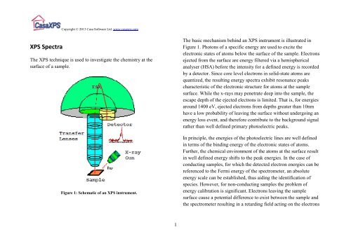
The <strong>XPS</strong> technique is used to investigate the chemistry at the<br />
surface of a sample.<br />
Figure 1: Schematic of an <strong>XPS</strong> instrument.<br />
1<br />
The basic mechanism behind an <strong>XPS</strong> instrument is illustrated in<br />
Figure 1. Photons of a specific energy are used to excite the<br />
electronic states of atoms below the surface of the sample. Electrons<br />
ejected from the surface are energy filtered via a hemispherical<br />
analyser (HSA) before the intensity for a defined energy is recorded<br />
by a detector. Since core level electrons in solid-state atoms are<br />
quantized, the resulting energy spectra exhibit resonance peaks<br />
characteristic of the electronic structure for atoms at the sample<br />
surface. While the x-rays may penetrate deep into the sample, the<br />
escape depth of the ejected electrons is limited. That is, for energies<br />
around 1400 eV, ejected electrons from depths greater than 10nm<br />
have a low probability of leaving the surface without undergoing an<br />
energy loss event, and therefore contribute to the background signal<br />
rather than well defined primary photoelectric peaks.<br />
In principle, the energies of the photoelectric lines are well defined<br />
in terms of the binding energy of the electronic states of atoms.<br />
Further, the chemical environment of the atoms at the surface result<br />
in well defined energy shifts to the peak energies. In the case of<br />
conducting samples, for which the detected electron energies can be<br />
referenced to the Fermi energy of the spectrometer, an absolute<br />
energy scale can be established, thus aiding the identification of<br />
species. However, for non-conducting samples the problem of<br />
energy calibration is significant. Electrons leaving the sample<br />
surface cause a potential difference to exist between the sample and<br />
the spectrometer resulting in a retarding field acting on the electrons
Copyright © 2013 Casa Software Ltd. www.casaxps.com<br />
escaping the surface. Without redress, the consequence can be peaks<br />
shifted in energy by as much as 150 eV. Charge compensation<br />
designed to replace the electrons emitted from the sample is used to<br />
reduce the influence of sample charging on insulating materials, but<br />
nevertheless identification of chemical state based on peak positions<br />
requires careful analysis.<br />
<strong>XPS</strong> is a quantitative technique in the sense that the number of<br />
electrons recorded for a given transition is proportional to the<br />
number of atoms at the surface. In practice, however, to produce<br />
accurate atomic concentrations from <strong>XPS</strong> spectra is not straight<br />
forward. The precision of the intensities measured using <strong>XPS</strong> is not<br />
in doubt; that is intensities measured from similar samples are<br />
repeatable to good precision. What may be doubtful are results<br />
reporting to be atomic concentrations for the elements at the surface.<br />
An accuracy of 10% is typically quoted for routinely performed <strong>XPS</strong><br />
atomic concentrations. For specific carefully performed and<br />
characterised measurements better accuracy is possible, but for<br />
quantification based on standard relative sensitivity factors,<br />
precision is achieved not accuracy. Since many problems involve<br />
monitoring changes in samples, the precision of <strong>XPS</strong> makes the<br />
technique very powerful.<br />
The first issue involved with quantifying <strong>XPS</strong> spectra is identifying<br />
those electrons belonging to a given transition. The standard<br />
approach is to define an approximation to the background signal.<br />
2<br />
The background in <strong>XPS</strong> is non-trivial in nature and results from all<br />
those electrons with initial energy greater than the measurement<br />
energy for which scattering events cause energy losses prior to<br />
emission from the sample. The zero-loss electrons constituting the<br />
photoelectric peak are considered to be the signal above the<br />
background approximation. A variety of background algorithms are<br />
used to measure the peak area; none of the practical algorithms are<br />
correct and therefore represent a source for uncertainty when<br />
computing the peak area. Peak areas computed from the background<br />
subtracted data form the basis for most elemental quantification<br />
results from <strong>XPS</strong>.<br />
Figure 2: An example of a typical <strong>XPS</strong> survey spectrum taken from a<br />
compound sample.
Copyright © 2013 Casa Software Ltd. www.casaxps.com<br />
The data in Figure 2 illustrates an <strong>XPS</strong> spectrum measured from a<br />
typical sample encountered in practice. The inset tile within Figure 2<br />
shows the range of energies associated with the C 1s and K 2p<br />
photoelectric lines. Since these two transitions include multiple<br />
overlapping peaks, there is a need to apportion the electrons to the C<br />
1s or the K 2p transitions using a synthetic peak model fitted to the<br />
data. The degree of correlation between the peaks in the model<br />
influences the precision and therefore the accuracy of the peak area<br />
computation.<br />
Relative sensitivity factors of photoelectric peaks are often tabulated<br />
and used routinely to scale the measured intensities as part of the<br />
atomic concentration calculation. These RSF tables can only be<br />
accurate for homogenous materials. If the sample varies in<br />
composition with depth, then the kinetic energy of the photoelectric<br />
line alters the depth from which electrons are sampled. It is not<br />
uncommon to see evidence of an element in the sample by<br />
considering a transition at high kinetic energy, but find little<br />
evidence for the presence of the same element when a lower kinetic<br />
energy transition is considered. Transitions of this nature might be<br />
Fe 2p compared to Fe 3p both visible in Figure 2, where the relative<br />
intensity of these peaks will depend on the depth of the iron with<br />
respect to the surface. Sample roughness and angle of the sample to<br />
the analyser also changes the relative intensity of in-homogenous<br />
samples, thus sample preparation and mounting can influence<br />
quantification values.<br />
3<br />
Figure 3: Germanium Oxide relative intensity to elemental germanium<br />
measured using photoelectrons with kinetic energy in the range 262 eV to 272<br />
eV.<br />
Figure 4: Germanium Oxide relative intensity to elemental germanium<br />
measured using photoelectrons with kinetic energy in the range 1452 eV to<br />
1460 eV.
Copyright © 2013 Casa Software Ltd. www.casaxps.com<br />
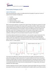
The chemical shifts seen in <strong>XPS</strong> data are a valuable source of<br />
information about the sample. The spectra in Figure 3 and Figure 4<br />
illustrate the separation of elemental and oxide peaks of germanium<br />
due to chemical state. Both spectra were acquired from the same<br />
sample under the same conditions with the exception that the ejected<br />
electrons for the Ge 3d peaks are about 1200 eV more energetic that<br />
the Ge 2p electrons. The consequence of choosing to quantify based<br />
on one of these transitions is that the proportion of oxide to<br />
elemental germanium differs significantly. The oxide represents an<br />
over layer covering of the elemental germanium and therefore the<br />
low energy photoelectrons from the Ge 2p line are attenuated<br />
resulting in a shallower sampling depth compared to the more<br />
energetic Ge 3d electrons. Hence the volume sampled by the Ge 2p<br />
transition favours the oxide signal, while the greater depth from<br />
which Ge 3d electrons can emerge without energy loss favours the<br />
elemental germanium. While these variations may seem a problem,<br />
such changes in the spectra are also a source for information about<br />
the sample.<br />
Tilting the sample with respect to the axis of the analyser results in<br />
changing the sampling depth for a given transition and therefore data<br />
collected at different angles vary due to the differing composition<br />
with depth. Figure 5 is a sequence of Si 2p spectra measured from<br />
the same silicon sample at different angles. The angles associated<br />
with the spectra are with respect to the axis of the analyser and the<br />
sample surface. Data measured at 30° favours the top most oxide<br />
4<br />
layers; while at 90° the elemental substrate becomes dominant in the<br />
spectrum.<br />
Figure 5: Angle resolved Si 2p spectra showing the changes to the spectra<br />
resulting from tilting the sample with respect to the analyser axis.
Copyright © 2013 Casa Software Ltd. www.casaxps.com<br />
Other Peaks in <strong>XPS</strong> <strong>Spectra</strong><br />
Not all peaks in <strong>XPS</strong> data are due to the ejection of an electron by a<br />
direct interaction with the incident photon. The most notable are the<br />
Auger peaks, which are explained in terms of the decay of a more<br />
energetic electron to fill the vacant hole created by the x-ray photon,<br />
combined with the emission of an electron with an energy<br />
characteristic of the difference between the states involved in the<br />
process. The spectrum in Figure 2 includes a sequence of peaks<br />
labelled O KLL. These peaks represent the energy of the electrons<br />
ejected from the atoms due to the filling of the O 1s state (K shell)<br />
by an electron from the L shell coupled with the ejection of an<br />
electron from an L shell.<br />
Unlike the photoelectric peaks, the kinetic energy of the Auger lines<br />
is independent of the photon energy for the x-ray source. Since the<br />
kinetic energy of the photoelectrons are given in terms of the photon<br />
energy , the binding energy for the ejected electron and a<br />
work function by the relationship , altering<br />
the photon energy by changing the x-ray anode material causes the<br />
Auger lines and the photoelectric lines to move in energy relative to<br />
one another.<br />
5<br />
Figure 6: Elemental Silicon loss peaks and also x-ray satellite peak.<br />
Less prominent than Auger lines are x-ray satellite peaks. Data<br />
acquired using a non-monochromatic x-ray source create satellite<br />
peaks offset from the primary spectral lines by the difference in<br />
energy between the resonances in the x-ray spectrum of the anode<br />
material used in the x-ray gun and also in proportion to the peaks in<br />
the x-ray spectrum for the anode material. Figure 6 indicates an<br />
example of a satellite peak to the primary Si 2p peak due to the use<br />
of a magnesium anode in the x-ray source. Note that Auger line<br />
energies are independent of the photon energy and therefore do not<br />
have satellite peaks.<br />
A further source for peaks in the background signal is due to<br />
resonant scattering of electrons by the surface materials. Plasmon
Copyright © 2013 Casa Software Ltd. www.casaxps.com<br />
peaks for elemental silicon are also labelled on Figure 6. The<br />
sharpness of these plasmon peaks in Figure 6 is due to the nature of<br />
the material through which the photoelectrons must pass. For silicon<br />
dioxide, the loss structures are much broader and follow the trend of<br />
a typical <strong>XPS</strong> background signal. The sharp loss structures in Figure<br />
6 are characteristic of pure metallic-like materials.<br />
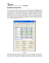
Basic Quantification of <strong>XPS</strong> <strong>Spectra</strong><br />
<strong>XPS</strong> counts electrons ejected from a sample surface when irradiated<br />
by x-rays. A spectrum representing the number of electrons recorded<br />
at a sequence of energies includes both a contribution from a<br />
background signal and also resonance peaks characteristic of the<br />
bound states of the electrons in the surface atoms. The resonance<br />
peaks above the background are the significant features in an <strong>XPS</strong><br />
spectrum shown in Figure 7.<br />
<strong>XPS</strong> spectra are, for the most part, quantified in terms of peak<br />
intensities and peak positions. The peak intensities measure how<br />
much of a material is at the surface, while the peak positions<br />
indicate the elemental and chemical composition. Other values, such<br />
as the full width at half maximum (FWHM) are useful indicators of<br />
chemical state changes and physical influences. That is, broadening<br />
of a peak may indicate: a change in the number of chemical bonds<br />
contributing to a peak shape, a change in the sample condition (x-ray<br />
6<br />
damage) and/or differential charging of the surface (localised<br />
differences in the charge-state of the surface).<br />
Figure 7: <strong>XPS</strong> and Auger peaks appear above a background of scattered electrons.<br />
Figure 8: Quantification regions
Copyright © 2013 Casa Software Ltd. www.casaxps.com<br />
The underlying assumption when quantifying <strong>XPS</strong> spectra is that the<br />
number of electrons recorded is proportional to the number of atoms<br />
in a given state. The basic tool for measuring the number of<br />
electrons recorded for an atomic state is the quantification region.<br />
Figure 8 illustrates a survey spectrum where the surface is<br />
characterised using a quantification table based upon values<br />
computed from regions. The primary objectives of the quantification<br />
region are to define the range of energies over which the signal can<br />
be attributed to the transition of interest and to specify the type of<br />
approximation appropriate for the removal of background signal not<br />
belonging to the peak.<br />
Figure 9: O 1s Region<br />
7<br />
How to Compare Samples<br />
A direct comparison of peak areas is not a recommended means of<br />
comparing samples for the following reasons. An <strong>XPS</strong> spectrum is a<br />
combination of the number of electrons leaving the sample surface<br />
and the ability of the instrumentation to record these electrons; not<br />
all the electrons emitted from the sample are recorded by the<br />
instrument. Further, the efficiency with which emitted electrons are<br />
recorded depends on the kinetic energy of the electrons, which in<br />
turn depends on the operating mode of the instrument. As a result,<br />
the best way to compare <strong>XPS</strong> intensities is via, so called, percentage<br />
atomic concentrations. The key feature of these percentage atomic<br />
concentrations is the representation of the intensities as a percentage,<br />
that is, the ratio of the intensity to the total intensity of electrons in<br />
the measurement. Should the experimental conditions change in any<br />
way between measurements, for example the x-ray gun power<br />
output, then peak intensities would change in an absolute sense, but<br />
all else being equal, would remain constant in relative terms.<br />
Relative Intensity of Peaks in <strong>XPS</strong><br />
Each element has a range of electronic states open to excitation by<br />
the x-rays. For an element such as silicon, both the Si 2s and Si 2p<br />
transitions are of suitable intensity for use in quantification. The rule<br />
for selecting a transition is to choose the transition for a given<br />
element for which the peak area, and therefore in principle the RSF,
Copyright © 2013 Casa Software Ltd. www.casaxps.com<br />
is the largest, subject to the peak being free from other interfering<br />
peaks.<br />
Transitions from different electronic states from the same element<br />
vary in peak area. Therefore, the peak areas calculated from the data<br />
must be scaled to ensure the same quantity of silicon, say, is<br />
determined from either the Si 2s or the Si 2p transitions. More<br />
generally, the peak areas for transitions from different elements must<br />
be scaled too. A set of relative sensitivity factors are necessary for<br />
transitions within an element and also for all elements, where the<br />
sensitivity factors are designed to scale the measured areas so that<br />
meaningful atomic concentrations can be obtained, regardless of the<br />
peak chosen.<br />
Figure 10: Regions Property Page.<br />
8<br />
Quantification of the spectrum in Figure 8 requires the selection of<br />
one transition per element. Figure 9 illustrates the area targeted by<br />
the region defined for the O 1s transition; similar regions are defined<br />
for the C 1s, N 1s and Si 2p transitions leading to the quantification<br />
table displayed over the data in Figure 8. The Regions property page<br />
shown in Figure 10 provides the basic mechanism for creating and<br />
updating the region parameters influencing the computed peak area.<br />
Relative sensitivity factors are also entered on the Regions property<br />
page. The computed intensities are adjusted for instrument<br />
transmission and escape depth corrections, resulting in the displayed<br />
quantification table in Figure 8.<br />
Quantification regions are useful for isolated peaks. Unfortunately<br />
not all samples will offer clearly resolved peaks. A typical example<br />
of interfering peaks is any material containing both aluminium and<br />
copper. When using the standard magnesium or aluminium x-ray<br />
anodes, the only aluminium photoelectric peaks available for<br />
measuring the amount of aluminium in the sample are Al 2s and Al<br />
2p. Both aluminium peaks appear at almost the same binding energy<br />
as the Cu 3s and Cu 3p transitions. Thus estimating the intensity of<br />
the aluminium in a sample containing these elements requires a<br />
means of modelling the data envelope resulting from the<br />
overlapping transitions illustrated in Figure 11.
Copyright © 2013 Casa Software Ltd. www.casaxps.com<br />
Figure 11: Aluminium and Copper both in evidence at the surface.<br />
Overlapping Peaks<br />
Techniques for modelling data envelopes not only apply to<br />
separating elemental information, such as the copper and aluminium<br />
intensities in Figure 11, but also apply to chemical state information<br />
about the aluminium itself. Intensities for the aluminium oxide and<br />
metallic states in Figure 11 are measured using synthetic line-shapes<br />
or components. An <strong>XPS</strong> spectrum typically includes multiple<br />
transitions for each element; while useful to identify the composition<br />
of the sample, the abundance of transitions frequently leads to<br />
interference between peaks and therefore introduces the need to<br />
9<br />
construct peak models. Figure 12 illustrates a spectrum where a thin<br />
layer of silver on silicon (University of Iowa, Jukna, Baltrusaitis and<br />
Virzonis, 2007, unpublished work) introduces an interference with<br />
the Si 2p transition from the Ag 4s transition.<br />
Figure 12: Elemental and oxide states of Silicon
Copyright © 2013 Casa Software Ltd. www.casaxps.com<br />
The subject of peak-fitting data is complex. A model is typically<br />
created from a set of Gaussian/Lorentzian line-shapes. Without<br />
careful model construction involving additional parameter<br />
constraints, the resulting fit, regardless of how accurate a<br />
representation of the data, may be of no significance from a physical<br />
perspective. The subject of peak fitting <strong>XPS</strong> spectra is dealt with in<br />
detail elsewhere.<br />
Peak models are created using the Components property page on the<br />
Quantification Parameters dialog window shown in Figure 13. A<br />
range of line-shapes are available for constructing the peak models<br />
including both symmetric and asymmetric functional forms. The<br />
intensities modelled using these synthetic line-shapes are scaled<br />
using RSFs and quantification using both components and regions<br />
are offered on the Report Spec property page of Casa<strong>XPS</strong>.<br />
Peak Positions<br />
In principle, the peak positions in terms of binding energy provide<br />
information about the chemical state for a material. The data in<br />
Figure 2 provides evidence for at least three chemical states of<br />
silicon. Possible candidates for these silicon states might be SiO2,<br />
Si2O3, SiO, Si2O or Si, however an assignment based purely on the<br />
measured binding energies for the synthetic line-shapes relies on an<br />
accurate calibration for the energy scale. Further, the ability to<br />
calibrate the energy scale is dependent on the success of the charge<br />
10<br />
compensation for the sample and the availability of a peak at known<br />
binding energy to provide a reference for shifting the energy scale.<br />
Figure 13: Components property page on the Quantification Parameters<br />
dialog window.<br />
Charge Compensation<br />
The <strong>XPS</strong> technique relies on electrons leaving the sample. Unless<br />
these emitted electrons are replaced, the sample will charge relative<br />
to the instrument causing a retarding electric field at the sample<br />
surface. For conducting samples electrically connected to the<br />
instrument, the charge balance is easily restored; however, for
Copyright © 2013 Casa Software Ltd. www.casaxps.com<br />
insulating materials electrons must be replaced via an external<br />
source. Insulating samples are normally electrically isolated from<br />
the instrument and low energy electrons and/or ions are introduced<br />
at the sample surface. The objective is to replace the photoelectrons<br />
to provide a steady state electrical environment from which the<br />
energy of the photoelectrons can be measured.<br />
Figure 14: Insulating sample before and after charge compensation.<br />
11<br />
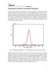
The data in Figure 14 shows spectra from PTFE (Teflon) acquired<br />
with and without charge compensation. The C 1s peaks are shifted<br />
by 162 eV between the two acquisition conditions, but even more<br />
importantly, the separation between the C 1s and the F 1s peaks<br />
differ between the two spectra by 5 eV. Without effective charge<br />
compensation, the measured energy for a photoelectric line may<br />
change as a function of kinetic energy of the electrons.<br />
Charge compensation does not necessarily mean neutralization of<br />
the sample surface. The objective is to stabilize the sample surface<br />
to ensure the best peak shape, whilst also ensuring peak separation<br />
between transitions is independent of the energy at which the<br />
electrons are measured. Achieving a correct binding energy for a<br />
known transition is not necessarily the best indicator of good charge<br />
compensation. A properly charge compensated experiment typically<br />
requires shifting in binding energy using the Calibration property<br />
page, but the peak shapes are good and the relative peak positions<br />
are stable.<br />
A nominally conducting material may need to be treated as an<br />
insulating sample. Oxide layers on metallic materials can transform<br />
a conducting material into an insulated surface. For example,<br />
aluminium metal oxidizes even in vacuum and a thin oxide layer<br />
behaves as an insulator.<br />
Calibrating spectra in Casa<strong>XPS</strong> is performed using the Calibration<br />
property page on the Spectrum Processing dialog window.
Copyright © 2013 Casa Software Ltd. www.casaxps.com<br />
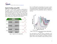
Depth Profiling using <strong>XPS</strong><br />
Figure 15: Segment of an <strong>XPS</strong> depth profile.<br />
While <strong>XPS</strong> is a surface sensitive technique, a depth profile of the<br />
sample in terms of <strong>XPS</strong> quantities can be obtained by combining a<br />
sequence of ion gun etch cycles interleaved with <strong>XPS</strong> measurements<br />
from the current surface. An ion gun is used to etch the material for<br />
a period of time before being turned off whilst <strong>XPS</strong> spectra are<br />
acquired. Each ion gun etch cycle exposes a new surface and the<br />
<strong>XPS</strong> spectra provide the means of analysing the composition of<br />
these surfaces.<br />
12<br />
Figure 16: The set of O 1s spectra measured during a depth profiling<br />
experiment.<br />
The set of <strong>XPS</strong> spectra corresponding to the oxygen 1s peaks from a<br />
depth profile experiment depicted logically in Figure 15 are<br />
displayed in Figure 16. The objective of these experiments is to plot<br />
the trend in the quantification values as a function of etch-time.<br />
The actual depth for each <strong>XPS</strong> analysis is dependent on the etch-rate<br />
of the ion-gun, which in turn depends on the material being etched at<br />
any given depth. For example, the data in Figure 16 derives from a<br />
multilayer sample consisting of silicon oxide alternating with<br />
titanium oxide layers on top of a silicon substrate. The rate at which
Copyright © 2013 Casa Software Ltd. www.casaxps.com<br />
the material is removed by the ion gun may vary between the layers<br />
containing silicon oxide and those layers containing titanium oxide,<br />
with a further possible variation in etch-rate once the silicon<br />
substrate is encountered. The depth scale is therefore dependent on<br />
characterizing the ion-gun however each <strong>XPS</strong> measurement is<br />
typical of any other <strong>XPS</strong> measurement, with the understanding that<br />
the charge compensation steady state may change between layers.<br />
Figure 17: <strong>XPS</strong> Depth Profile of silicon oxide/titanium oxide multilayer<br />
sample profiled using a Kratos Amicus <strong>XPS</strong> instrument.<br />
13<br />
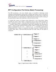
Figure 18: Logical structure of the VAMAS blocks in an <strong>XPS</strong> depth profile.<br />
The <strong>XPS</strong> depth profile in Figure 17 is computed from the VAMAS<br />
file data logically ordered in Casa<strong>XPS</strong> as shown in Figure 18. The O<br />
1s spectra displayed in Figure 16 are highlighted in Figure 18. One<br />
point to notice about the profile in Figure 17 is that the atomic<br />
concentration calculation for the O 1s trace is relatively flat for the<br />
silicon oxide and titanium oxide layers, in contrast to the raw data in<br />
Figure 16, where the chemically shifted O 1s peaks would appear to<br />
be more intense for the silicon oxide layers compared to the titanium<br />
oxide layers. This observation is supported by the plot of adjusted
Copyright © 2013 Casa Software Ltd. www.casaxps.com<br />
peak areas in Figure 19, where again the O 1s trace is far from flat.<br />
The profile in Figure 17 is far more physically meaningful than the<br />
variations displayed in Figure 19. Normalization of the <strong>XPS</strong><br />
intensities to the total signal measured on a layer by layer basis is<br />
important for understanding the sample. This example is a good<br />
illustration of why <strong>XPS</strong> spectra should be viewed in the context of<br />
the other elements measured from a surface.<br />
The details of how to analyze a depth profile in Casa<strong>XPS</strong> are<br />
discussed at length in The Casa Cookbook and other manual pages<br />
available from the Help option on the Help menu.<br />
Figure 19: Peak areas scaled by RSF used to compute the atomic<br />
concentration plots in Figure 17.<br />
14<br />
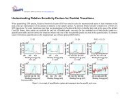
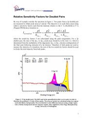
Understanding Relative Sensitivity Factors for<br />
Doublet Transitions<br />
When quantifying <strong>XPS</strong> spectra, Relative Sensitivity Factors (RSF)<br />
are used to scale the measured peak areas so variations in the peak<br />
areas are representative of the amount of material in the sample<br />
surface. An element library typically contains lists of RSFs for <strong>XPS</strong><br />
transitions. For some transitions more than one peak appears in the<br />
data in the form of doublet pairs and, in the case of the default<br />
Casa<strong>XPS</strong> library, three entries are available for each set of doublet<br />
peaks: one entry for the combined use of both doublet peaks in a<br />
quantification table and two entries for situations where only one of<br />
the two possible peaks are used in the quantification. A common<br />
cause of erroneous quantification is the inappropriate use of these<br />
optional RSF entries.<br />
Figure 20: Example of quantification regions and components used to<br />
quantify peak areas.
Copyright © 2013 Casa Software Ltd. www.casaxps.com<br />
The data in Figure 20 are a set of high resolution spectra where<br />
quantification regions and components are used to calculate the area<br />
for the peaks. These data illustrate some of the issues associated<br />
with <strong>XPS</strong> quantification as the data includes singlet peaks in the<br />
form of O 1s, C 1s, Al 2s and N 1s; as well as doublet pairs: Cr 2p,<br />
Cu 2p, Ar 2p and Fe 2p. The spectra are sufficiently complex to<br />
involve overlaps such as the Al 2s and Cu 3s, while the Cu 2p1/2<br />
peak includes signal from a Cr Auger line. When creating a table of<br />
percentage atomic concentrations it is important to select the correct<br />
RSF for the peak area chosen to measure the given element.<br />
Name R.S.F. % Conc.<br />
Cr 2p 1/2 10.6041 2.9<br />
Cr 2p 3/2 10.6041 6.2<br />
Fe 2p 1/2 14.8912 2.2<br />
Fe 2p 3/2 14.8912 4.5<br />
Cu 2p 3/2 15.0634 4.4<br />
Al 2s Metal 0.753 61.4<br />
Al 2s Ox 0.753 5.1<br />
Ar 2p 2.65797 5.5<br />
O 1s 2.93 6.2<br />
C1s 1 1.5<br />
N1s 1.8 0.2<br />
Table 1: Quantification table showing RSFs used to scale the raw peak areas.<br />
When measuring a transition, from the perspective of signal to noise,<br />
it is better to include both peaks from a doublet pair. For the data in<br />
Figure 20, the Fe 2p, Cr 2p and Ar 2p transitions are free of<br />
15<br />
interference from other peaks and therefore simple integration<br />
regions can be used to measure the peak areas. The Ar 2p doublet<br />
peaks overlap each other; however the Cr 2p and Fe 2p peaks do not<br />
overlap, thus separate quantification regions are used to measure the<br />
area for these resolved doublet peaks. Even though separate regions<br />
are used to estimate the peak areas for the two peaks in each of the<br />
Cr 2p and the Fe 2p transitions, total RSFs for these transitions are<br />
used to scale the raw area calculated from the regions. Similarly, the<br />
total RSF is used to scale the Ar 2p doublet peaks, because both<br />
peaks from the doublet are used in calculating the peak area for<br />
argon. On the other hand, since the Cu 2p1/2 peak overlaps with the<br />
Cr LMM Auger transition, only the Cu 2p3/2 peak can be used with<br />
ease and so the reduced RSF must be applied to scale the peak area.<br />
The quantification table in Table 1 lists the regions and components<br />
used to calculate the atomic concentrations together with the RSFs<br />
for each transition.<br />
Note the peak model used to measure the Al 2s includes a<br />
component representing the contribution of the Cu 3s transition to<br />
the Al 2s spectrum in Figure 20. Copper is measured using the Cu<br />
2p3/2 peak therefore the RSF for the Cu 3s component is set to zero<br />
so that the component does not appear in Table 1.<br />
By way of example, an alternative quantification regime might be to<br />
use only one of the two possible Fe 2p doublet peaks. The<br />
quantification in Table 2 removes the Fe 2p1/2 region from the
Copyright © 2013 Casa Software Ltd. www.casaxps.com<br />
calculation by setting the RSF to zero, whilst adjusting the Fe 2p3/2<br />
RSF to accommodate the absence of the Fe 2p1/2 peak area from the<br />
calculation. Since the ratio of 2p doublet peaks should be 2:1, the<br />
RSF for the Fe 2p3/2 region is two thirds of the total RSF used in<br />
Table 1. In Table 1, the percentage atomic concentration for Fe is<br />
split between the two Fe 2p doublet peaks, whereas in Table 2 the<br />
entire Fe 2p contribution is estimated using the Fe 2p3/2 and<br />
therefore the same amount of Fe is measured via either approach.<br />
A common misunderstanding is to use both peaks in the calculation,<br />
but still assign RSFs for the individual peaks in the doublet. The<br />
consequence of using both peaks and the specific RSFs to the<br />
individual peaks in the doublet is the contribution from Fe to the<br />
quantification table would be incorrectly increased by a factor of<br />
two.<br />
Note: the RSFs used in both Table 1 and Table 2 are Scofield crosssections<br />
adjusted for angular distribution corrections for an<br />
instrument with angle of 90º between the analyser and x-ray source.<br />
Name R.S.F. % Conc.<br />
Cr 2p 1/2 10.6041 2.9<br />
Cr 2p 3/2 10.6041 6.2<br />
Fe 2p 3/2 9.8064 6.8<br />
Cu 2p 3/2 15.0634 4.4<br />
16<br />
Al 2s Metal 0.753 61.3<br />
Al 2s Ox 0.753 5.1<br />
Ar 2p 2.65797 5.5<br />
O 1s 2.93 6.2<br />
C1s 1 1.5<br />
N1s 1.8 0.2<br />
Table 2: Fe 2p 3/2 peak is used without the area from the Fe 2p1/2.<br />
To further illustrate the issues associated with the uses of the three<br />
RSFs associated with doublet peaks, consider the three possible<br />
options available when quantifying the Cr 2p doublet shown in<br />
Figures 21, 22 and 23. Table 3 shows that the corrected area when<br />
measured using any of these three options is approximately the<br />
same.<br />
Figure 21: Intensity for Cr calculated from the Cr 2p1/2 transition.<br />
Cr 2p1/2 RSF Raw Area<br />
3.60721 19234.8
Copyright © 2013 Casa Software Ltd. www.casaxps.com<br />
Figure 22 Intensity for Cr calculated from the Cr 2p3/2 transition.<br />
Cr 2p3/2 RSF Raw Area<br />
6.9697 40871.9<br />
Figure 23 Intensity for Cr calculated from both peaks in the doublet.<br />
Total RSF Raw Area<br />
10.6041 60098.5<br />
17<br />
Peak<br />
RSF Raw Area Corrected Area<br />
Raw Area/(RSF*T*MFP)<br />
Cr 2p 1/2 3.60721 19234.8 125.455<br />
Cr 2p 3/2 6.9697 40871.9 138.192<br />
Both Cr 2p Peaks 10.6041 60098.5 133.555<br />
Table 3: Comparison of the intensities calculated from the three different<br />
combinations of peak area and RSF for the Cr 2p doublet illustrated in<br />
Figure 21 Figure 22 and Figure 23.<br />
Electronic Energy Levels and <strong>XPS</strong> Peaks<br />
An electron spectrum is essentially obtained by monitoring a signal<br />
representing the number of electrons emitted from a sample over a<br />
range of kinetic energies. The energy for these electrons, when<br />
excited using a given photon energy, depends on the difference
Copyright © 2013 Casa Software Ltd. www.casaxps.com<br />
between the initial state for the electronic system and the final state.<br />
If both initial and final states of the electronic system are well<br />
defined, a single peak appears in the spectrum. Well defined<br />
electronic states exist for systems in which all the electrons are<br />
paired with respect to orbital and spin angular momentum. The<br />
initial state for the electronic system offers a common energy level<br />
for all transitions. When an electron is emitted from the initial state<br />
due to the absorption of a photon, the electrons emerge with kinetic<br />
energies characteristic of the final states available to the electronic<br />
system and therefore <strong>XPS</strong> peaks represent the excitation energies<br />
open to the final states. Since these final states include electronic<br />
sub-shells with unpaired electrons, the spin-orbit coupling of the<br />
orbital and spin angular moment results in the splitting of the energy<br />
levels otherwise identical in terms of common principal and orbital<br />
angular momentum. Thus, instead of a single energy level for a final<br />
state, the final state splits into two states referred to in <strong>XPS</strong> as<br />
doublet pairs. To differentiate between these <strong>XPS</strong> peaks, labels are<br />
assigned to the peaks based on the hole in the final state electronic<br />
configuration. Since these final states, even when split by spin-orbit<br />
interactions, are still degenerate in the sense that more than one<br />
electronic state results in the same energy for the system, three<br />
quantum numbers are sufficient to identify the final state for the xray<br />
excited system. Specifying the three quantum numbers in the<br />
format nlj both uniquely identifies the transition responsible for a<br />
18<br />
peak in the spectrum and offers information regarding the<br />
degeneracy of the electronic state involved. The relative intensity of<br />
these doublet pair peaks linked by the quantum numbers nl is<br />
determined from the j = l ± ½ quantum number. Doublet peaks<br />
appear with intensities in the ratio 2j1+1 : 2j2+1. Thus p-orbital<br />
doublet peaks are assigned j quantum numbers 1/2 and 3/2 and appear<br />
with relative intensities in the ratio 1:2.<br />
Similar intensity ratios and differing energy separations are common<br />
features of doublet peaks in <strong>XPS</strong> spectra. Final states with s<br />
symmetry do not appear as doublets, e.g. Au 4s.
Copyright © 2013 Casa Software Ltd. www.casaxps.com<br />
Examples of <strong>XPS</strong> <strong>Spectra</strong><br />
19
Copyright © 2013 Casa Software Ltd. www.casaxps.com<br />
Bulk molybdenum disulphide measured using a Kratos Axis Nova<br />
20
Copyright © 2013 Casa Software Ltd. www.casaxps.com<br />
21
Copyright © 2013 Casa Software Ltd. www.casaxps.com<br />
C<br />
O<br />
C<br />
H<br />
C<br />
O<br />
H<br />
Tartaric Acid<br />
H<br />
C<br />
C<br />
O<br />
H<br />
O<br />
C<br />
C<br />
O<br />
H<br />
Carbon appears in tartaric acid in two<br />
chemical environments resulting in two<br />
identifiable binding energies for the C 1s<br />
transition. Each chemical state appears<br />
in equal proportions in the tartaric acid<br />
molecule.<br />
O<br />
22<br />
H<br />
H<br />
O<br />
O<br />
O<br />
C<br />
C
Copyright © 2013 Casa Software Ltd. www.casaxps.com<br />
O<br />
C<br />
Oxygen appears in the tartaric acid molecule in<br />
two chemical environments resulting in two<br />
closely positioned binding energies for the O 1s<br />
transition. Each chemical state appears in a<br />
proportion of 2:4 in the tartaric acid molecule.<br />
23<br />
C<br />
O<br />
H
Copyright © 2013 Casa Software Ltd. www.casaxps.com<br />
24
Copyright © 2013 Casa Software Ltd. www.casaxps.com<br />
SiO2 measured using an aluminium anode.<br />
25
Copyright © 2013 Casa Software Ltd. www.casaxps.com<br />
Note the relative movement of the O KLL Auger line relative to the O 1s peak for data acquired using a magnesium anode compared<br />
to the SiO2 data measured with an aluminium anode. The elemental silicon in the sample also accounts for the sequence of plasmon<br />
loss peaks not seen in the SiO2 data.<br />
26
Copyright © 2013 Casa Software Ltd. www.casaxps.com<br />
Aluminium oxide sample analysed using an aluminium monochromatic source.<br />
27
Copyright © 2013 Casa Software Ltd. www.casaxps.com<br />
Again, metallic aluminium is responsible for the sequence of plasmon loss peaks associated with the Al 2p and Al 2s photoelectric<br />
lines not present in the aluminium oxide spectrum. It is worth observing the argon from the ion gun used to reduce the depth of the<br />
aluminium oxide layer exhibits plasmon loss structures characteristic of the aluminium metal. Note also that the plasmon loss peaks<br />
from the Al 2p transition will interfere with the Al 2s peak, hence the common practice of using the Al 2p line to quantify samples<br />
containing aluminium.<br />
28
Copyright © 2013 Casa Software Ltd. www.casaxps.com<br />
Gold measured using a silver anode in the x-ray monochromatic source.<br />
29
Copyright © 2013 Casa Software Ltd. www.casaxps.com<br />
Gold spectrum measured using a Cylindrical Sector Analyser (CSA) and Synchrotron a photon energy of 10.5 keV (PETRA P09 Beamline,<br />
Hamburg DESY; FOCUS HV-CSA).<br />
30
Copyright © 2013 Casa Software Ltd. www.casaxps.com<br />
31
Copyright © 2013 Casa Software Ltd. www.casaxps.com<br />
32
Copyright © 2013 Casa Software Ltd. www.casaxps.com<br />
33
Copyright © 2013 Casa Software Ltd. www.casaxps.com<br />
34
Copyright © 2013 Casa Software Ltd. www.casaxps.com<br />
35
Copyright © 2013 Casa Software Ltd. www.casaxps.com<br />
36
Copyright © 2013 Casa Software Ltd. www.casaxps.com<br />
37
Copyright © 2013 Casa Software Ltd. www.casaxps.com<br />
38
Copyright © 2013 Casa Software Ltd. www.casaxps.com<br />
39
Copyright © 2013 Casa Software Ltd. www.casaxps.com<br />
40
Copyright © 2013 Casa Software Ltd. www.casaxps.com<br />
41
Copyright © 2013 Casa Software Ltd. www.casaxps.com<br />
42
Copyright © 2013 Casa Software Ltd. www.casaxps.com<br />
43
Copyright © 2013 Casa Software Ltd. www.casaxps.com<br />
44
Copyright © 2013 Casa Software Ltd. www.casaxps.com<br />
45
Copyright © 2013 Casa Software Ltd. www.casaxps.com<br />
46
Copyright © 2013 Casa Software Ltd. www.casaxps.com<br />
47
Copyright © 2013 Casa Software Ltd. www.casaxps.com<br />
Data provided by Bridget Rogers, Vanderbilt University, Nashville, TN, USA<br />
48
Copyright © 2013 Casa Software Ltd. www.casaxps.com<br />
49
Copyright © 2013 Casa Software Ltd. www.casaxps.com<br />
50
Copyright © 2013 Casa Software Ltd. www.casaxps.com<br />
51
Copyright © 2013 Casa Software Ltd. www.casaxps.com<br />
52
Copyright © 2013 Casa Software Ltd. www.casaxps.com<br />
53
Copyright © 2013 Casa Software Ltd. www.casaxps.com<br />
54
Copyright © 2013 Casa Software Ltd. www.casaxps.com<br />
55
Copyright © 2013 Casa Software Ltd. www.casaxps.com<br />
56
Copyright © 2013 Casa Software Ltd. www.casaxps.com<br />
The peak model is to illustrate a complex data envelope fitted with simple Gaussian-Lorentzian lineshapes. For a more complete<br />
discussion of Ce Oxide please see:V. Matolín, M. Cabala, V. Cháb, I. Matolínová, K. C. Prince, M. Škoda, F. Šutara, T. Skála and K.<br />
Veltruská, A resonant photoelectron spectroscopy study of Sn(Ox) doped CeO2 catalysts, Surf. Interface Anal. 40 (2008) 225–230.<br />
57
Copyright © 2013 Casa Software Ltd. www.casaxps.com<br />
58
Copyright © 2013 Casa Software Ltd. www.casaxps.com<br />
59
Copyright © 2013 Casa Software Ltd. www.casaxps.com<br />
60
Copyright © 2013 Casa Software Ltd. www.casaxps.com<br />
61
Copyright © 2013 Casa Software Ltd. www.casaxps.com<br />
62
Copyright © 2013 Casa Software Ltd. www.casaxps.com<br />
<strong>XPS</strong> spectra and electronic structure of Group IA sulfates, M. Wahlqvist, A. Shchukarev / Journal of Electron Spectroscopy and<br />
Related Phenomena 156–158 (2007) 310–314<br />
<strong>XPS</strong> Study of Group IA Carbonates, A.V. Shchukarev, D.V. Korolkov / CEJC 2(2) 2004 347-362<br />
63
Copyright © 2013 Casa Software Ltd. www.casaxps.com<br />
64
Copyright © 2013 Casa Software Ltd. www.casaxps.com<br />
65
Copyright © 2013 Casa Software Ltd. www.casaxps.com<br />
66
Copyright © 2013 Casa Software Ltd. www.casaxps.com<br />
67
Copyright © 2013 Casa Software Ltd. www.casaxps.com<br />
68
Copyright © 2013 Casa Software Ltd. www.casaxps.com<br />
69
Copyright © 2013 Casa Software Ltd. www.casaxps.com<br />
70
Copyright © 2013 Casa Software Ltd. www.casaxps.com<br />
71
Copyright © 2013 Casa Software Ltd. www.casaxps.com<br />
72
Copyright © 2013 Casa Software Ltd. www.casaxps.com<br />
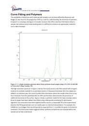
PMMA<br />
CH<br />
2<br />
C<br />
C<br />
O<br />
CH3<br />
C<br />
C<br />
O<br />
CH3<br />
O<br />
n<br />
O<br />
H<br />
C H<br />
Different Chemical States for Carbon in Poly(methyl methacrylate)<br />
O<br />
H<br />
C<br />
73<br />
C<br />
C<br />
C<br />
C<br />
H<br />
C<br />
H<br />
C<br />
C<br />
H<br />
C<br />
H<br />
H<br />
C
Copyright © 2013 Casa Software Ltd. www.casaxps.com<br />
Poly(methyl methacrylate): C 1s peak assignments are based on those of Beamson and Briggs (The <strong>XPS</strong> of Polymers Database<br />
Edited by Graham Beamson and David Briggs (2000) ISNB: 0-9537848-4-3.<br />
74
Copyright © 2013 Casa Software Ltd. www.casaxps.com<br />
75
Copyright © 2013 Casa Software Ltd. www.casaxps.com<br />
76
Acknowledgments<br />
Copyright © 2013 Casa Software Ltd. www.casaxps.com<br />
Data used to prepare this PDF were donated by:<br />
University of Manchester, UK<br />
University of Nottingham, UK<br />
Peking University, China<br />
Max Plank Institute Düsseldorf, Germany<br />
Umeå University, Sweden<br />
Lehigh University, USA<br />
Vanderbilt University, Nashville, TN, USA<br />
Technical University of Eindhoven, The Netherlands<br />
University of Nantes, France<br />
and several unnamed contributors.<br />
A thank you to all involved in collecting these data.<br />
77