Dynamic SIMS - CasaXPS

CasaXPS Manual 2.3.15 Rev 1.0 

Copyright © 2010 Casa Software Ltd 

CasaXPS Manual 2.3.15 

CasaXPS Processing Software 

Casa Software Ltd. 

NO WARRANTY 

Casa Software Ltd. does its best to ensure the accuracy and reliability of the Software and 

Related Documentation. Nevertheless, the Software and Related Documentation may 

contain errors that may affect its performance to a greater or lesser degree. Therefore no 

representation is made nor warranty given that the Software and Related Documentation 

will be suitable for any particular purpose, or that data or results produced by the 

Software and Related Documentation will be suitable for use under any specific 

conditions, or that the Software and Related Documentation will not contain errors. Casa 

Software Ltd. shall not in any way be liable for any loss consequential, either directly or 

indirectly, upon the existence of errors in the Software and Related Documentation. The 

Software and Related Documentation, including instructions for its use, is provided “AS IS” 

without warranty of any kind. Casa Software Ltd. further disclaims all implied warranties 

including without limitation any implied warranties of merchantability or fitness for a 

particular purpose. CasaXPS should not be relied on for solving a problem whose incorrect 

solution could result in injury to a person or loss of property. The entire risk arising out of 

the use or performance of the Software and Related Documentation remains with the 

Recipient. In no event shall Casa Software Ltd. be liable for any damages whatsoever, 

including without limitation, damages for loss of business profit, business interruption, 

loss of business information or other pecuniary loss, arising out of the use or inability to 

use the Software or written material, even if Casa Software Ltd. has been advised of the 

possibility of such damages. 

Acknowledgements 

Casa Software Ltd would like to thank all those providing data and offering 

enlightening discussions leading to the current state of the CasaXPS software 

and manual. It is a humbling experience to work with so many knowledgeable 

people and the author would like to express gratitude to all concerned. 

1



Contents 

CasaXPS Processing Software ............................................................................................................ 1 

Casa Software Ltd. ........................................................................................................................... 1 

NO WARRANTY ............................................................................................................................... 1 

Acknowledgements ............................................................................................................................. 1 

The Nature of ToF Spectra ................................................................................................................... 5 

ToF Mass Calibration ........................................................................................................................... 7 

Calibration Based on Nominal Masses ............................................................................................ 9 

An Example of Mass Calibration using Nominal Masses ........................................................... 11 

Recalibration of Mass Scale for ToF Spectra ..................................................................................... 15 

Recalibration Steps ........................................................................................................................ 17 

Peak Fitting ToF SIMS Data ................................................................................................................ 18 

Line-shapes Suitable for ToF SIMS Spectra ................................................................................... 19 

Peak Identification and Reduction .................................................................................................... 21 

IonToF Peak Identification ................................................................................................................. 23 

Converting IonToF Spectra ................................................................................................... 24 

Directory Profiling ......................................................................................................................... 26 

Profile Directory Toolbar Option ...................................................................................... 28 

Working with ToF Spectra in CasaXPS ............................................................................................... 29 

Time to Mass Calibration Procedures ........................................................................................... 29 

Mass Calibration using Regions and Propagation of Regions between Spectra ....................... 30 

Mass Calibration ........................................................................................................................ 31 

Propagation of Calibration Regions ........................................................................................... 31 

Mass Calibration using the Exact Mass Calculator Property Page: ........................................... 33 

The Element Library from a ToF Perspective ................................................................................ 35 

The Element Library and Linking ToF Peaks for Display ............................................................ 36 

Profiling Features for ToF data .......................................................................................................... 47 

ToF Data File Options .................................................................................................................... 49 

Create a Total Ion Spectrum ............................................................................................. 50 

Create Images from Spectra using Quantification Regions ....................................................... 52 

Spectra Generated from Image Zones ...................................................................................... 54 

Creating a Profile from a Total Ion Spectrum ............................................................................ 56 

Spectra Generated from Profile Layers ............................................................................. 58 

2



Create a Profile from a Directory of Files .......................................................................... 58 

Convert and Merge a Directory of XYT File ....................................................................... 61 

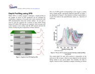
Image Depth Profile Data Analysis .............................................................................. 63 

Quantification Reports and ToF Data ................................................................................................ 66 

Quantification via the Report Spec Property Page ....................................................................... 66 

Standard Report ........................................................................................................................ 67 

Custom Report .......................................................................................................................... 70 

An Overview of Working with ToF Data in CasaXPS ......................................................................... 72 

SIMS Toolbar Buttons: Display Options ........................................................................................ 72 

An Overview .................................................................................................................................. 79 

Basics of CasaXPS .......................................................................................................................... 81 

Converting Data ........................................................................................................................ 81 

Data Viewed Via an Experiment Frame .................................................................................... 82 

Displaying Data .......................................................................................................................... 83 

Selecting VAMAS Blocks ............................................................................................................ 84 

Tile Display Options ................................................................................................................... 85 

Display Colours .......................................................................................................................... 86 

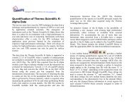
Calculating SNMS Sensitivity Factors ............................................................................................ 88 

Quantification of SNMS Profiles .................................................................................................... 98 

Quantification of Stainless Steel using SNMS: an Example ....................................................... 98 

Specifying the Sputter-Rate .................................................................................................... 103 

Creating a Calibrated SNMS Profile ......................................................................................... 104 

Dynamic SIMS .................................................................................................................................. 109 

Notes on Dynamic SIMS RSF Calculation .................................................................................... 110 

Reference Signal Measured during the Course of Profile ....................................................... 110 

Reference Signal Measured at End of Acquisition Cycles ....................................................... 111 

Quantification of Dynamic SIMS Profiles .................................................................................... 112 

Quantification of Basic Profiles ............................................................................................... 114 

Making Adjustments to the Sputter Rate ............................................................................... 125 

Display of Calibrated Profiles .................................................................................................. 126 

Further Aspects of Dynamic SIMS Quantification ....................................................................... 127 

Logical Structure of a SIMS Depth Profile within CasaXPS ...................................................... 127 

Methods for Computation of RSF and Sputter Rate Values ................................................... 128 

Identification of the Matrix and Interface Cycles.................................................................... 128 

3



Selecting Ranges of Cycles on the Calibration Property Page ................................................. 132 

Surface Data and Background Signal ....................................................................................... 133 

Three Ways to Calculate RSF Values from Standard Samples ................................................. 134 

Adding RSF and Sputter Rates to Profile Data ......................................................................... 135 

Applying Calibration Parameters to One or More Profiles...................................................... 135 

Depth Profile Statistics: Areal Density and Decay Length ....................................................... 136 

Maintaining Standards Library Files ........................................................................................ 137 

Step-by-Step Description of Quantification for a Multi-Layer Sample .................................... 137 

An Example of Computing an RSF using Dose and Implant Peak Depth ................................. 143 

Computing RSFs where the Matrix Signal is Measured following the Completion of the Implant 

Profile ...................................................................................................................................... 145 

Gathering Profile Data for Display and Calibration Purposes ..................................................... 147 

4



TOF SIMS 

The Nature of ToF Spectra 

Time-of-Flight Mass Spectrometry (ToF MS) is based on the principle that ions 

created from a sample are accelerated into a flight tube using an electric 

extraction field resulting in each ion of a given charge acquiring a 

characteristic energy from a tight distribution of possible energies. Since the 

kinetic energy of the ions are nearly identical, the velocity attained by ions 

with differing mass must also differ, thus the time taken for an ion with a 

given charge to travel a given distance down the flight tube to the detector 

discriminates between ions of different mass. Specifically, the mass of an ion 

is proportional to the square of the time taken to travel a fixed distance. 

Thus, ToF MS works on the basis of a stop-watch; a start event occurs as the 

extraction voltage is pulsed, followed by a sequence of stop events 

representing the arrival of ions at the detector. To process a ToF mass 

spectrum from the raw timing data, a histogram is created from the set of 

time values, where the time events recorded during an experiment are 

counted into time-bins. The relationship between the time events and the 

mass of the ions responsible for the time events allows the time-bin 

histogram to be viewed using a mass scale. 

CasaXPS displays the ToF intensities with respect to the time bin indices, even 

when a mass calibration is available. Converting a spectrum to mass binned 

intensities involves a mapping which cannot be reversed; explicit steps must 

be taken to perform the transformation between time and mass. 

The following two plots are for the same data, both viewed in the time 

domain. The mass range in these two plots is identical. 

5



The same spectrum plotted using a linear mass step size changes the 

perspective of the data as follows. 

Spectra from ToF instruments traditionally appear as a single spectrum over a 

wide range of mass. The spectral display reflects the parallel nature of the 

technique in the sense that counts are allocated over the entire range of time 

bins for each pulse of the ion gun. This is in contrast to quadrupole or 

magnetic sector MS instruments where the signal is only recorded one mass 

bin at a time. Nevertheless, for high resolution ToF MS the majority of time 

bins, particularly at low mass, contain little information, therefore CasaXPS 

offers a means of converting ToF spectra from a single monolithic data set 

into a set of mass intervals representative of the useful information content. 

Each nominal mass, based on the current time to mass calibration, is isolated 

into individual VAMAS blocks. Presenting a ToF spectrum as a set of many 

6



VAMAS blocks favours the tools within CasaXPS providing the basis for data 

comparison and peak analysis via synthetic peak models. 

The partitioning of the time bins into suitable mass ranges around the 

nominal masses requires a calibration for the mass scale. 

ToF Mass Calibration 

The relationship between the mass m of an ion and the time taken for the ion 

of a given charge to travel a fixed distance is quadratic in the flight time t. For 

an ideal system, the time-to-mass relationship is: 

m 

[( t t b 

2 

0 

) / ] 

where t 0 represents a time offset and b scales the time values appropriately. 

Since knowledge of these two parameters t 0 and b is sufficient to describe 

the relationship between the mass and time-of-flight, given two mass/time 

pairs the calibration parameters can be determined from a pair of 

simultaneous equations. In reality, assigning the mass/time coordinates from 

the time-binned spectra is not exact and therefore the time-to-mass 

calibration must be computed in a least-squares sense using multiple 

mass/time pairs. Further, the choice of mass/time pairs must be carefully 

made to ensure accuracy of the calibration for both interpolated and 

extrapolated mass regions. Those mass regions falling within (interpolation) 

the set of mass/time pairs used to create the calibration will be more 

accurate with respect to the time-to-mass calibration than those outside 

(extrapolation) the interval containing the mass/time pairs included in the 

7



least squares fit. It is therefore important to calibrate a spectrum using peaks 

over as wide a mass range as possible and check that peaks, once calibrated, 

can be sequentially assigned to nominal masses. The following describes the 

tools in CasaXPS for calibrating a spectrum of time-bins with respect to mass 

and how to assess the success of this procedure. 

Figure 1 

Figure 2: An example of a poor mass calibration based on extrapolation. 

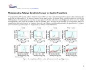
When calibrating the mass scale, the primary objective is to assign each 

visible peak to a nominal mass. For some spectra and instruments, there may 

be perfectly good reasons why this objective may fail, but in general each 

peak in the data should be associated with a nominal mass; any mass defect 

from the nominal mass provides information about the atomic or molecular 

ion responsible for the peak. It is not necessary nor is it always possible to 

attribute each peak to a known ion, however, when properly calibrated, if the 

observable peaks deviate from the sequence of nominal masses then the 

accuracy of the calibration may be in doubt. The problem of calibrating the 

mass scale reduces to identifying a set of peaks sufficiently well distributed 

over the mass scale to provide plausible mass assignments for each and every 

8



peak in the spectrum. Figure 1 is an example of a mass calibration in which 

the set of peaks displayed matches well with the computed mass positions; 

however the calibration is performed using only those peaks within the 

window in Figure 1 and a similar agreement, when using the same 

calibration, for the molecules shown in Figure 2 is not achieved. The poor 

mass calibration is remedied by simply including at least one of the peaks in 

Figure 2 as part of the calibration set. The concept of progressively adding 

calibration points to the set used to mass calibrate a spectrum is developed 

in following sections. 

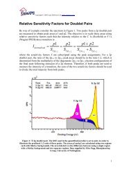
Calibration Based on Nominal Masses 

Figure 3: Nominal mass calibration 

The procedure for calibrating a spectrum can be summarised as follows: 

following an initial assignment based on at least two peaks, new peaks are 

progressively added to the set of mass/time pairs until the observed peaks 

are sequentially associated with nominal masses. The spectrum in Figure 3 is 

calibrated based on nominal masses and an iterative improvement 

procedure. This process can be performed manually using the Exact Mass 

property page (Figure 4), where peaks are associated with formulae using the 

mouse, or alternatively nominal masses are used in a sequence of steps 

involving repeatedly: 

1. Finding the peaks using the Find Peaks button. 

9



2. Replacing the current calibration list by nominal masses and times 

determined from the regions obtained from the Find Peak operation. 

The Load Regions button transfers the required information from the 

current set of regions to the calibration list on the Exact Mass property 

page. 

3. Recalibrate the mass scale by pressing the Calib C,t0 button. 

Figure 4: Exact Mass Calculator Property Page. 

The Find Peaks button uses a threshold to identify peak structures in the 

data; then for each peak identified, a region is created on the spectrum using 

the name derived from the nominal mass determined from the region. The 

Load Regions button transfers those nominal mass names and computed 

positions to the calibration table on the Exact Mass property page for which 

the computed mass is within a tolerance of the nominal mass. The search for 

these acceptable mass/time pairs begins with the low masses, so the initial 

calibration should begin with small masses, but typically greater than 10 amu. 

With each repetition of these steps, the number of regions loaded into the 

calibration table should increase until, ideally, all the peaks found are 

included in the calibration table. At this point, the spectrum so calibrated 

should be surveyed to ensure the peaks, both minor and major, are 

associated with the nominal masses on the abscissa scale. 

10



Figure 5: Raw time-binned spectrum. 

Calibration using nominal mass values is not always appropriate, for example 

heavy molecular ions; however, for some spectra, calibration using exact 

masses is equally inappropriate. The data in Figure 1 is an example of a 

spectrum for which it is beneficial to use nominal masses rather than exact 

masses; the spectrum derives from a total ion list file containing image 

information and minor variations in acquisition conditions across the imaged 

surface cause small shifts in the underlying peaks summed to form the total 

ion spectrum. Peaks are neither high enough in mass resolution nor well 

enough defined in terms of position to use an exact mass position. The latter 

can be demonstrated using false colour images to extract spectra from 

different zones on the image. 

An Example of Mass Calibration using Nominal Masses 

Initially the spectrum is without a mass calibration as seen in Figure 5. The 

first step is to identify two peaks. 

Figure 6: Two peaks are identified by creating quantification regions. 

11



The regions defined on the spectrum in Figure 6 represent the initial pair of 

mass/time coordinates used to produce a rough calibration for the mass 

scale. The regions are created using the Regions property page on the 

Quantification Parameters dialog window. Each region calculates the timebin 

representative of the peak, while the mass corresponding to the 

computed time-bin is entered into the name field of the quantification 

region. In this case, the name fields are entered with the nominal masses 15 

and 23, although these values could equally well have been entered using the 

formulae C+H*3 and Na, respectively. Calibration based on these two regions 

is performed by pressing the toolbar button. When the toolbar button is 

pressed, any spectra appearing in the Active Tile will be calibrated based on 

regions so defined on the displayed spectra. 

Figure 7: Spectrum after initial mass calibration. 

While the calibration in Figure 7 looks reasonable for masses close to the 

calibration points, the high mass peaks are poorly calibrated. The largest 

peak in Figure 8 differs by about 18 amu from the mass calibration shown in 

Figure 3. 

Figure 8: Poor mass calibration for high mass peaks. Same peaks as those displayed using the 

inset tile in Figure 3. 

12



While the initial mass calibration based to only two low mass peaks is clearly 

a problem at higher masses, the accuracy is sufficient to begin the iterative 

process of build a fuller set of mass calibration points. 

Figure 9: Exact Mass property page. 

Figure 10: Result of Find Peaks with a threshold of 20. 

Given the initial mass calibration based on the peaks labelled 15 and 23, the 

Find Peaks button on the Exact Mass property page shown in Figure 9 can be 

used to assign nominal masses to all peaks characterized by a threshold 

value. On pressing the Find Peaks button, a dialog window appears in which a 

threshold value can be entered. In the case of the results shown in Figure 10 

the threshold value was set to 20. Once a new set of regions are created 

using the Find Peaks button, the Load Regions button is pressed, the 

consequence of which is the mass calibration table on the Exact Mass 

property page is loaded with the set of calibration points determined from 

the regions currently defined on the spectrum, subject to the condition that 

the mass determined from the time bin for each region is within a tolerance 

of the nominal mass entered into the name field of the region. Following the 

13



initial mass calibration and application of the Find Peaks button, the set of 

regions generated by the Find Peaks button in Figure 10 are limited by the 

Load Regions button to those displayed in Figure 9. That is, all regions above 

nominal mass 31 were sufficiently different from the nominal mass to be 

rejected. The deviation of the computed mass for peaks above 31 amu from 

the nominal mass is a measure of the error in the original mass calibration. 

Given the new set of calibration points, the Calib button on the Exact Mass 

property page can be pressed resulting in an improved mass calibration. 

Repeating the Find Peaks operation followed by reloading the regions into 

the calibration table reveals that peaks up to 53 amu are now included in the 

calibration table. A third iteration of these steps produced a calibration table 

including peaks up to 228 amu, while a forth iteration extends the calibration 

table up to 561 amu, exhausting the set of peaks found using the Find Peaks 

button. The mass calibration based on nominal masses is now complete. All 

that remains is to verify the mass calibration by stepping through the spectral 

peaks to confirm the presence of peaks at each amu and that known peaks 

are correctly assigned. 

Figure 11: High resolution ToF peaks clearly distinct from the nominal mass of 28 amu. 

The procedure is not without flaw, so verification is necessary, but can 

provide a means of improving an initial calibration with minimal effort. For 

high resolution ToF spectra, the use of nominal masses will lead to a rough 

mass scale which requires refinement using resolved peaks and exact mass 

formulae (Figure 11). 

NB: The peak marker in Figure 11 for elemental Si is positioned to the lefthand 

side of the peak. When a ToF spectrum is calibrated using the option on 

the toolbar, the position of peaks with respect to time are determined from 

the regions. While the peak maximum may appear to be a good choice for 

14



the peak position, the asymmetry typically observed in ToF peaks and the 

variety of peak shapes over a spectrum suggest, in general, the peak 

maximum is less well defined than the leading edge of a peak. For this 

reason, the position of the peak used for the calibration procedure is taken to 

be the lower full width half maximum. Hence the peak markers will align with 

the leading edge of the peaks rather than the peak maxima. Note that the 

calibration option on the Exact Mass property page offers the choice of peak 

position to the user without limitation. 

Recalibration of Mass Scale for ToF Spectra 

Occasionally ToF Spectra are supplied as mass binned data. While data in 

mass bins is convenient for those without the ability to handle the relatively 

large time binned spectra, the possibility exists that the mass calibration used 

to mass-bin the spectra may not be accurate enough for the application in 

question. For high resolution mass spectra, a small error in the original timeto-mass 

calibration may lead to the type of uncertainty illustrated in Figure 

12, where the peak maximum falls between the two most likely assignments 

for the measured data. A recalibration of the mass bins is therefore required. 

Figure 12: An example of a mass-binned spectrum where the original mass calibration is not 

sufficiently accurate for the resolution of the peak shown. 

The recalibration of mass-binned data differs from a time-to-mass calibration 

of time-binned data in that the act of reallocating the counts to mass-bins 

from the original time-binned data (performed during the creation of the 

mass spectrum), results in the loss of information. Namely, two or more 

time-bins may map into the same mass-bin, therefore it is impossible to take 

a mass-bin and repopulate the time-bins with the same distribution found in 

the original data set. The consequence of there being a fundamental 

15



difference between these two operations is that, when recalibrating a massbinned 

spectrum, the functional form used to assign the data bins to mass 

values must involve a general three parameter quadratic function rather than 

the stiffer model used to calibrate time-bins to mass-bins. The two parameter 

calibration function recommended for time-to-mass calibration is too specific 

to the counting mechanism used to acquire the ToF MS data. The extra 

flexibility offered by the three parameter quadratic is needed to model the 

errors in the original time-to-mass calibration; the stiffer two-parameter 

quadratic model used for time-to-mass calibration is dictated by and 

appropriate to the physics of the ToF instrument. 

While CasaXPS allows time-to-mass calibration using both the recommended 

two-parameter quadratic model and the general three-parameter quadratic 

function, the same warning about the three-parameter functional form is 

equally applicable to both situations. That is, the flexibility offered by the 

general quadratic function allows non-physical solutions for the mass 

assignment of peaks. It is possible to create a mass calibration when using 

the three-parameter quadratic for which known peaks are apparently 

correctly assigned to masses, yet other peaks in the spectrum are incorrectly 

assigned. Extrapolation based on the three parameter model should be 

viewed with suspicion. Ideally, ToF MS data should be provided in the time 

domain, nevertheless situations do occur where mass-binned data must be 

managed and therefore CasaXPS provides a mean of recalibrating the massbinned 

data. Figure 13 shows the same data seen in Figure 12 following the 

recalibration procedure described below. 

Figure 13: The same mass spectrum after recalibration. 

16



Recalibration Steps 

1. Cancel the Mass calibrated status of the spectra: overlay the massbinned 

spectra in the Active Tile and press the toolbar button on 

the SIMS toolbar. The label for the abscissa will return to “Time Bin”, 

which indicates the data is in a state where a new calibration can be 

created. Note, the abscissa values will be bin indices, not true timebins, 

but nevertheless it is necessary to the calibration procedure that 

the abscissa label is assigned the string “Time Bin”. 

2. Using the Exact Mass Calculator, a new calibration set defining the 

relationship between the peaks and the mass assignment must be 

established. The procedure is identical to creating a time-to-mass 

calibration described elsewhere. 

3. Perform the recalibration using the button on the Exact Mass 

Calculator property page of the Element Library dialog window. 

Figure 14: A mass-binned peak illustrating the peak deformations due to the re-binning 

algorithm used to create the mass spectrum. 

An alternative procedure is to create quantification regions and apply the 

recalibration using the toolbar button. While possible, this approach 

suffers from the information lost during the time-to-mass conversion 

procedure, that is, the mass-bins for higher mass values tend to be poorly 

defined compared to the original time data (Figure 14). The algorithms for 

identifying a peak position and therefore determining the calibration points 

17



assumes the data obeys Passion statistics, but otherwise varies smoothly; it is 

clear from Figure 14 that the mass-binned data contains anomalous values. 

Peak Fitting ToF SIMS Data 

The features in CasaXPS typically used to model XPS data envelopes can also 

be used to analyst overlapping peaks in high resolution ToF SIMS spectra. The 

principal difference between ToF SIMS and XPS is that asymmetry in ToF 

SIMS peaks is, in general, in the opposite direction to that found for XPS 

peaks. As a result, not all line-shapes in CasaXPS are appropriate for ToF SIMS 

peaks, however the more recently introduced asymmetric line-shapes of LA 

and LF provide a means of creating line-shapes appropriate for the range of 

ToF SIMS peaks observed in practice. 

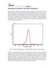
The data in Figure 15 illustrates the similarities between XPS and ToF SIMS, 

where the mass peaks associates with a nominal mass of 42 are very typical 

of polymer XPS spectra such as PMMA or PET. The problems of 

understanding the data are also similar in that both the position and the 

intensity of the underlying peaks are of importance when identifying the 

molecular ions responsible for the measured data. 

Figure 15: Example of ToF SIMS peak structure. 

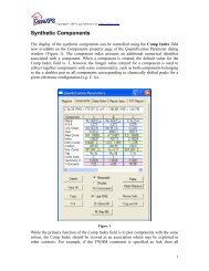
The procedure for adding synthetic components to the data involves first 

adding a quantification region to the data with background type set of “Zero” 

before adding synthetic line-shapes. Creating and adjusting regions and 

components is performed on the Quantification Parameters dialog window 

18



available from the Quantify option on the Options menu or the toolbar 

button on the top toolbar of CasaXPS. Regions and components are managed 

using the tables found on the Regions and Components property pages of 

the Quantification Parameters dialog window shown in Figure 16. 

The peaks shown in Figure 15 are defined using the parameters displayed in 

the table on the Components property page illustrated in Figure 16. The lineshape 

parameter in this example is defined using the LA functional form, 

where the parameters provide a degree of asymmetry to the right of the 

peak maximum. The meaning of these parameters is described below. 

Figure 16: Quantification Dialog Window. 

Line-shapes Suitable for ToF SIMS Spectra 

The success of a peak fit is dependent on an appropriate choice for the lineshape 

parameter. As stated above, the LA and LF line-shapes offer sufficient 

flexibility for most ToF SIMS peak shapes. 

The Lorentzian line-shape with FWHM F and position M is given by 

1 

L ( x : f , e) 

(1) 

2 

x e 

1 4 

f 

The functional form is symmetrical about x = M. In order to retain the 

characteristics of the Lorentzian line-shape and yet also introduce 

asymmetry, the LA line-shape is defined in two halves as 

19



LA(α,β,m): Equation (2) defines the first two parameters used in the lineshape 

LA(α,β,m) shown in Figure 16. The third parameter m is used to 

control the width of a Gaussian convolution applied to the functional form 

defined by Equation (2). As a consequence of the definition for the LA lineshape, 

an asymmetry line-shape is established by specifying α not equal to β. 

Further, is α is greater than β then the resulting peak will be asymmetric with 

an extended tail to the right of the peak maximum. Adjusting the Gaussian 

convolution parameter causes the extent of the asymmetric tail to reduce 

and also shifts the peak maximum towards the extended tail. 

LF(α, β, w, m): Identical to the LA line-shape with the exception that the 

specified values of α and β are force to increase to a constant value via a 

smooth function determined by the width parameter w. The w parameter is 

used to restrict the extent of the tail. 

(2) 

Figure 17: Asymmetric Mass Peak fitted using a single LA line-shape. 

By way of example, the elemental sodium mass peak shown in Figure 17 

exhibits significant asymmetry to the right of the peak maximum, which can 

be modelled using the LA line-shape. Note that the line-shape included in the 

annotation of the peak in Figure 17 is achieved by setting the first parameter 

to a value greater than unity, thus compressing the tail to the left compared 

20



to the tail to the right. Further, the Lorentzian tail to the right of the peak 

maximum is adjusted by convoluting the functional shape with a Gaussian of 

characteristic width described by a value of 250 for the m parameter in the 

LA definition. The degree of asymmetry is determine by the relative size of 

the first parameter compared to the second, that is α > β. 

Figure 18 

The line-shape used in Figure 17 should be compared with the line-shape in 

Figure 18 corresponding to a similar sodium peak measured using the same 

IonToF instrument but using a different ion gun. The peak in Figure 18 rises 

more quickly than the peak in Figure 17, therefore the α-parameter is now 

much larger than the β-parameter, which is also set to a value greater than 

unity. The larger the values for these two parameters the steeper the edge of 

the peak appears. Also note in Figure 18 that the Gaussian convolution is 

much narrower than that used in Figure 17. Possible values for the Gaussian 

parameter are between 0 and 499; m = 0 corresponds to no convolution 

being performed. 

Peak Identification and Reduction 

High resolution ToF spectra typically consist of numerous peaks, however for 

some analyses only a small number of correlated peaks are significant for 

21



distinguishing between samples. That is, a peak at one mass is only 

characteristic of a particular compound when also accompanied by peaks at a 

set of very specific masses. Given the plethora of peaks typically present in 

ToF MS data, a means of grouping and displaying only significant peaks is 

required. To visualise the spectrum with respect to only significant peaks, a 

ToF spectrum can be organised in CasaXPS 2.3.15 such that the Element 

Library property page simplifies the mechanism by which these significant 

peaks can be displayed for visual inspection. In addition to the element 

marks, a spectrum can be broken into an array of VAMAS blocks representing 

the peak information associated with the nominal masses and the element 

library used to display appropriate subsets of these VAMAS blocks for 

interpretation. 

The procedure for splitting a ToF spectrum into a set of mass calibrated 

VAMAS blocks can be performed using the toolbar button indicated in Figure 

19. As an alternative approach, for data files for which a mass calibration is 

available to CasaXPS at the time of conversion the division of the data into 

mass calibrated VAMAS blocks can be performed at the time the data are 

converted. Either route to the mass calibrated VAMAS blocks requires a mass 

calibration for the data. 

Figure 19: ToF Spectrum with data in time domain. 

22



The data in Figure 19 are converted to a mass calibrated set of VAMAS blocks 

by pressing the toolbar button with hint Split into Unit Mass Spectra. The 

result of converting the data in Figure 19 is shown in Figure 20, where the 

right-hand pane displays the set of VAMAS blocks derived from the single 

VAMAS block in Figure 19. 

The display in Figure 20 is achieved by overlaying the full set of VAMAS blocks 

from the right-hand pane in the active tile. An inset tile is used to display a 

specific VAMAS block, namely the VAMAS block corresponding to a nominal 

mass of 42. Note that since the individual VAMAS blocks are mass calibrated, 

the overlay appears in the form of a mass calibrated spectrum. 

Figure 20: ToF Spectrum after conversion to mass calibrated VAMAS blocks. 

The discussion that follows relates to data prepared in the format shown in 

Figure 20. Presenting the spectrum as a set of VAMAS block provides the 

basis for the tools within CasaXPS. Before describing these tools, the method 

for converting data files directly to mass calibrated sets of VAMAS blocks will 

be addressed. Version 2.3.15 of CasaXPS only offers data conversion to the 

multiple VAMAS block format for ASCII files formatted using the convention 

adopted by the IonToF data system. 

IonToF Peak Identification 

IonToF spectra are exported in ASCII files in the format shown in Figure 21. 

The follow describes the options in CasaXPS for importing these data in 

formats suitable for compiling peak lists. 

23



Figure 21:IonToF ASCII format. 

The SIMS toolbar in CasaXPS offers two toolbar buttons for controlling the 

import of data in the format shown in Figure 21. These toolbar buttons are 

indicated in Figure 22. 

Figure 22: SIMS Toolbar buttons 

The traditional method for working with ToF data is based on a single data 

block approach, however the tools for peak identification now added to 

CasaXPS are organized on a partitioning of the data into numerous data 

blocks based on the nominal mass for each group of peaks. The objective is to 

analyze a directory of spectra and determine a set of mass peaks and 

intensities for each spectrum in the directory. 

Converting IonToF Spectra 

Figure 23: ASCII txt files exported from the IonToF software. 

24



A data directory initially contains a set of spectra exported from the IonToF 

software as ASCII txt files. Figure 23 illustrates such a directory which is 

displayed using the File Dialog window offered by the toolbar button. The 

conversion of these data may be performed using several filter strings as 

follows: 

1. “.ion” 

2. “.amu” 

3. “.sum”. 

To initiate a conversion sequence, a name followed by one of the above 

strings must be entered into the File name text-field on the File Dialog in 

Figure 23. For example, to convert and merge the set of txt files in a format 

suitable for peak identification, the File name text-field should be entered 

with the string “datafile.amu”. The base-name is arbitrary, however the 

extension “.amu” instructs the set of txt files to be converted to VAMAS 

format (a new VAMAS file will appear in the directory for each txt file 

processed) then these converted files are merged into a single experiment 

frame in CasaXPS. Note that these data are large; therefore the process is 

both time consuming and requires plenty of PC memory! 

The different filter strings determine the nature of the data files generated 

from the IonToF ASCII files. The individual VAMAS files generated from the 

ASCII files are identical for both the “.amu” and “.sum” filters; the final 

outcome differs however, where the “.amu” filter causes the merger of the 

spectra into a single experiment frame as separate spectra equivalent to the 

original ASCII data, while the “.sum” filter results in the total counts from the 

set of spectra in the ASCII files forming the equivalent of a single mass 

spectrum. In both cases, the mass spectrum from each of the IonToF files is 

partitioned into VAMAS blocks corresponding to data in the vicinity of the 

nominal mass values. Figure 24 shows the result of using the “.sum” filter on 

the data directory depicted in Figure 23. Both display tiles in Figure 24 display 

an overlay of all the data blocks in the right-hand pane of the experiment 

frame and the inset tile shows the data from the three highlight blocks 

containing intensities for nominal masses 41, 42 and 43 amu. 

25



Figure 24: Example of a total counts spectrum formed from the four ASCII files shown in 

Figure 23. 

The conversion filter “.ion” when applied to a directory merges the data into 

a single experiment frame containing one spectrum per original ASCII file, but 

maintains the data for each spectrum as a single block. While the format 

adopted is more traditional for mass spectra, the peak identification option 

uses peak-fitting and therefore the format shown in Figure 24 is more suited 

to the algorithms involved. The single block of data provided by the “.ion” is 

for visual inspection of the full data set and should not be used when peak 

identification is employed. 

Directory Profiling 

The objective addressed by the features described here, is to identify and 

quantify in terms of mass assignments and intensities the set of peaks 

characteristic of a sample. The peak structures within a ToF spectrum are 

illustrated in Figure 25, where it can be seen that at least five overlapping 

peaks to varying degrees are responsible for the data envelope. Peak 

intensity and peak position are determined for these types of peak structures 

using optimized peak modelling. The very fact that peak modelling is required 

highlights the difficulty of automatically identifying all the peaks for a given 

data envelope. For a directory of similar spectra, automatically identifying 

mass peaks from data such as that in Figure 25 is fraught with dangers and 

therefore the strategy in CasaXPS for processing directories of similar spectra 

is one of aiding the construction of a template spectrum, for which peak 

models are prepared to be exhaustive with respect to the data under 

analysis, then the automatic application of the template models to a 

26



directory of spectra forms the basis for extracting the quantitative 

information for each spectrum in the directory. 

Figure 25: Mass peak structure from a ToF spectrum. 

The creation of peak models for each significant mass peak in a file such as 

the one shown in Figure 24 is central to the profiling options in CasaXPS. 

About 500 data blocks corresponding to the nominal masses potentially 

require the construction of regions and synthetic peaks. The success of the 

template approach relies on the peak models adequately describing the 

peaks with appropriate constraints in terms of relative positions and FWHM 

to permit the peak intensities to be calculated from the fitted model. To 

assist this initial step, an option on the Exact Mass Calculator property page 

of the Element Library dialog window offers a means of creating peak models 

based on a threshold limit. 

The Create Peaks button on the Exact Mass Calculator property page (Figure 

26) uses the threshold value to limit the number of peaks created for a given 

data block. 

Figure 26: Exact Mass Calculator Property page. 

27



The peak creation mechanism uses the threshold value entered on the MS 

Peak Threshold dialog window to create a region and synthetic peaks for 

each data block overlaid in the active tile. The smaller the threshold values, 

the smaller the peaks will be that are included in the peak search. Since the 

significance of mass peaks may not depend entirely on peak intensity, it is 

worth noting that different threshold values may be appropriate for different 

ranges in the mass scale. It is therefore unlikely that a single application of 

the Create Peaks button will generate all the appropriate peaks, however, by 

the user selectively overlaying data blocks and choosing different thresholds, 

peaks can be created on large numbers of data blocks while still retaining the 

discretion of the operator. Ultimately, the success or failure of the profiling 

step will depend on the way these peak models are constructed and time 

spent in getting these models right will be recovered by the accuracy and 

automatic application of these models to larger data directories. 

Profile Directory Toolbar Option 

The options for profiling a directory of IonToF spectra are as follows: 

1. “.amu” 

2. “.fit” 

3. “.vfc” 

These conversion filters are used to control the nature of the directory 

profile. On providing a base name followed by one of these filter strings, the 

directory located by the File Dialog window invoked by the toolbar button 

is scanned for the appropriate file types and, on accepting the Continue 

prompt via the resulting message dialog, the set of files are one-by-one 

processed to produce several text file reports and a VAMAS file containing 

the profile information from the directory. 

The two profile filters “.amu” and “.fit” both require a template spectrum to 

be loaded and displayed in the active tile. In the case of the “.amu” profile 

filter, the ASCII .txt IonToF files are converted to VAMAS files before applying 

the template information to these newly converted data, which are also 

saved in the processed state as .vms files. On completion, several text files 

provide the results of the profile, one offering the context information for the 

numerical tabulations located in the other files. In addition, the profile 

information is presented in VAMAS format within the current CasaXPS 

session. 

28



The second profile filter “.fit” performs the same sequence of steps as the 

“.amu” with the exception that the files processed from the directory are the 

“.vms” files. This removes the conversion step from the operation and is 

appropriate if, for example, the data directory has been previously processed 

using the “.sum” conversion filter described above. The “.sum” conversion 

filter generates a single spectrum from a set of files in a directory and also, as 

part of the process, converts the ASCII files to VAMAS format. The total 

counts spectrum created from the “.sum” operation may appear in the same 

directory as the converted files, but provided the filename retains the “.sum” 

sub-string, the total spectrum will not appear in the final profile results 

generated from applying the template file to the set of .vms files in the 

current directory. 

An alternative way to profile a directory of .vms files is to apply the “.vfc” 

profile filter. In this case, no fitting is performed, but rather the existing peak 

fits within the set of VAMAS files is used to construct the profile information. 

The “.vfc” profile filter allows the individual files to be inspected and any 

anomalies rectified on a file-by-file basis before creating the profile 

information. It is important that the same set of VAMAS blocks and number 

of synthetic peaks are used on each of the data blocks, however profiling the 

directory without automatic peak fitting allows user-intervention to override 

poor fitting scenarios. 

Working with ToF Spectra in CasaXPS 

Time to Mass Calibration Procedures 

A raw ToF spectrum is recorded in the time domain. Mass calibration of a ToF 

spectrum is performed in CasaXPS by identifying a set of peaks in the data 

with specific masses; then, by using these pairs of mass/time values a 

quadratic relationship between the time and mass scales is created. A linear 

least squares procedure determines the two constants within the quadratic 

expression and therefore two or more mass/time pairs must be supplied to 

perform the calibration procedure. The accuracy of the mass-to-time 

calibration is dependent of the precision of the mass/time pairs used in the 

least squares calculation; the more pairs used to compute the least squares 

solution, the more tolerant the calibration will be to errors in the mass/time 

specification. 

29



CasaXPS offers two methods for calibrating ToF MS data: 

1. Peaks and corresponding masses specified using quantification regions. 

2. Mouse identification of the peaks coupled with an exact mass 

calculator located on the Element Library dialog window. 

Mass Calibration using Regions and Propagation of Regions 

between Spectra 

The Quantification Parameters Dialog window provides a means of 

defining time intervals, within which systematic positions are defined 

(computed from a peak bounded by an interval) and linked to masses via an 

exact mass formula entered into the Name field for the regions. 

Figure 27: Quantification Parameters Dialog Window shown three regions defined for the 

purpose of calibrating the time scale to mass. 

The spectrum in Figure 27 is an example of ToF SIMS data where three 

quantification regions are defined suitable for calibrating the time scale to 

mass. The mass associated with each region is entered into the Name field 

and may be a numerical value exemplified by the region headed column B or 

a string corresponding to any exact mass formula equivalent to expressions 

use on the Exact Mass property page of the Element Library dialog window. 

30



For example, the mass of a peak might be defined using the expression 

C+H*3, which when evaluated would result in a mass of 15.0235 Daltons. 

Mass Calibration 

One or more time domain spectra can be prepared with calibration regions as 

described above and overlaid in the active tile in the left-hand pane of the 

experiment frame. On pressing the toolbar button, each spectrum in the 

active tile is calibrated using the peaks within the regions. Since multiple 

spectra can be mass calibrated using a single invocation of the toolbar 

button, the use of this procedure is supported by the propagation of the 

calibration regions to similar spectra, thus avoiding the need to manually 

create regions for each spectrum requiring a mass calibration. 

Propagation of Calibration Regions 

The procedure to propagate the calibration regions from the spectrum as 

defined in Figure 27 to two other similar spectra is as follows: 

1. Select the VAMAS blocks in each of the two experiment frames 

containing the spectra requiring the calibration regions. 

The CasaXPS window is arranged in a tiled format using the Tile option from 

the Window menu at the top of the CasaXPS main window. The arrangement 

of the experiment frames allows the selection to be made by left-clicking the 

first VAMAS block in the experiment frame to the bottom-left and then 

holding the Control-Key down and left-clicking the VAMAS block in the 

bottom-right experiment frame 

31



2. The Browser Operations dialog window is invoked by right-clicking the 

mouse with the cursor over the left-hand pane of the top-most 

experiment frame. The objective is to right-click over the display tile in 

which the spectrum containing the calibration regions is displayed. 

3. To propagate regions to the two selected VAMAS blocks, which are 

listed on the Browser Operations dialog window, tick the radio button 

in the Propagate section of the dialog window and press the OK 

button. Region labels are now visible on the spectra. 

The data in each of the three experiment frames are calibrated by switching 

focus between the experiment frames and each time pressing the toolbar 

32



button. Control-TAB moves the focus between the experiment frames within 

CasaXPS. 

The time to mass calibration for the time domain data may be seen labelling 

the x-axis using a quadratic mass scale. 

Mass Calibration using the Exact Mass Calculator Property Page: 

The procedure for calibrating a spectrum involves creating a set of 

mass/time-bin pairs within the scrolled-list on the Exact Mass property page 

on the Element Library dialog window. 

The example below illustrates how the columns in the scrolled-list headed 

Mass and Time store the information relating these two parameters. Before 

an assignment for a given entry has been made, the value in the Time column 

is set to -1. The mass for an entry in the table is computed from the chemical 

formula entered into the name column. 

33



To add an entry to the calibration table: 

1. Type a chemical formula into the text-field below the scrolled list and 

press the Add Formula button or press the return key on the keyboard. 

The formula for an ion may be entered using the chemical symbols 

used to on the Periodic Table property page of the Element Library 

dialog window. 

2. Select the name in the scrolled-list. To select a name field, place the 

cursor over the text within the Name column and left-click the mouse. 

The name entry will appear highlighted when successfully selected. 

3. Zoom into the known peak in the spectrum displayed in the active tile. 

It is important to perform the zoom operation before step 4 is taken. 

4. Tick the tick-box labelled “Define Time”. 

5. Using the mouse cursor, click on the known peak at a location 

representative of the mass already defined by the selected entry in the 

scrolled list. The value in the Time column is updated and the Define 

Time tick-box is cleared. 

At least two entries must be specified in the scrolled-list before pressing the 

Calib C,t0 button on the Exact Mass property page. The more entries 

assigned mass/time pairs, the better the mass to time calibration will be 

computed in the least squares sense. 

Once a calibration table has been prepared, a file containing the calibration 

points can be saved to a separate text file from the data. 

34



These files can be reloaded at a later time to provide an initial calibration for 

other data or for making adjustments to the calibration of the original 

spectrum used to create the calibration file. Note, while the Save button on 

the Exact Mass property page saves the current calibration table, the Load 

button will merge a saved file with the current set of entries on the scrolledlist. 

To return the table to the entries within a file, it is first necessary to press 

the Delete All button. The Delete All button removes the current entries in 

the scrolled-list, while the Delete Entry button removes the currently 

selected entry. 

If an assignment is incorrect, the individual entry must be deleted from the 

table. The name field for the deleted entry is entered into the text field 

below the scrolled list; therefore a selected entry can be deleted then 

reinstated by immediately pressing the Add Formula button. The Time field 

will return to a value of -1 and therefore be ignored during any subsequent 

calibration operation. 

The Element Library from a ToF Perspective 

The element library in CasaXPS is an ASCII file. On startup, CasaXPS loads the 

default element library from within the same directory as the one in which 

the CasaXPS.exe executable file is located. The name of the default element 

35



library file is CasaXPS.lib and is designed with the view that the element 

library can be constructed for specific applications. For example, in the case 

of quadrupole MS, a library consisting of elemental isotopes is appropriate to 

the resolution of quadrupole mass spectra, while for high resolution ToF MS 

a library consisting of entries for molecular fragments is required when 

assigning mass peaks. 

Preparing an element library file for mass spectra may be performed using a 

spreadsheet program such as Excel or tools on the Exact Mass Calculator 

property page allowing correctly formatted library files to be constructed 

from lists of chemical formulae. Methods for displaying the significant peaks 

based on selections from an element library constructed from one or more 

library files are described below. 

The Element Library and Linking ToF Peaks for Display 

High resolution ToF spectra typically consist of numerous peaks; however for 

some analyses only a small number of correlated peaks are significant for 

distinguishing between samples; a peak at one mass is only characteristic of a 

particular compound when also accompanied by other peaks in the 

spectrum. A strong link between the element library and displaying data for 

inspection is therefore introduced in CasaXPS 2.3.15. The objective is to use 

the element library to specify a set of mass peaks grouped with respect to 

correlated peaks which are used to makes selections of VAMAS blocks. These 

selections of VAMAS blocks containing narrow interval mass spectra combine 

with the display tools in CasaXPS to provide a perspective in which overall 

spectral distribution and localised peak structure can be assessed with 

relative ease. 

A ToF data set presented as a set of unit mass VAMAS blocks can be viewed 

in the more traditional form of a single plot. The traditional perspective of a 

ToF spectrum is achieve by selecting all the VAMAS blocks in the right-hand 

pane, then pressing the overlay toolbar button. When viewed as a single 

continuous display, all the features for manipulating the display are still open 

for use. 

36



The advantage of creating a set of mass calibrated VAMAS files is that the 

spectrum can be dissected and displayed with a variety of options: 

Display only those peaks more than 5% in intensity of the largest peak. 

Display one VAMAS block per tile for those peaks greater than 5% of the 

maximum peak. All peaks scaled with respect to a specific peak; mass 23 in 

this case. 

37



Scale the peaks on an individual basis. 

Take a closer look at specific peaks. 

Enhancements for manipulating the selection and display for ToF MS data are 

available on the Element Table property page of the Element Library dialog 

window. 

38



The mechanisms offered on the Element Table property page are described 

in the following sections. 

Linking Element Library Entries 

A CasaXPS library file may be prepared with a set of entries corresponding to 

particular sample chemistry. Such a library file can be loaded or merged with 

the existing library file whenever appropriate. The essential feature of the 

entries in the given library file is that a set of mass formulae are all assigned 

the same unique string for the Transition column. 

Using the Selection Mechanism 

By way of example, a set of formulae only involving carbon and hydrogen are 

assigned the Transition string CH. On selecting one of the entries using the 

Name column of the table on the Element Table property page bearing the 

CH Transition string before pressing the Display Linked VBs button on the 

Element Table property page causes all those VAMAS blocks (in the 

experiment frame with focus) to be displayed in the left-hand pane, one 

VAMAS block per tile. Thus, a set of related mass peaks can be easily 

displayed for inspection. 

39



A dialog window provides a means of only selecting those VAMAS blocks for 

which the peak intensity is greater than the specified percentage of the 

maximum peak in the data. 

The key used to match the VAMAS blocks in the experiment frame is the 

string corresponding to the Species VAMAS field within each VAMAS block. 

The Species VAMAS field is used in the header string for each column of 

blocks in the right-hand pane of the experiment frame. 

The ToF spectral files, when split into sets of VAMAS blocks, are created using 

the appropriate nominal masses to create these Species fields and the library 

entries with the common Transition library field are used to compute the 

corresponding nominal mass for each library entry, which when matched to 

the Species VAMAS fields causes the data to be displayed in the tile list. 

40



The element library file also includes Transition strings CO and F. 

The different assignments for the Transition strings are simply a partition of 

the file between three possible sets of mass peaks; however a more realistic 

example might involve significant peaks from any combination of mass peaks, 

all of which would be collectively assigned a common Transition string. 

Should the same mass peak correspond to more than one compound, the 

element library file can include repeated entries differing only by the 

Transition string. 

Overlaying Related VAMAS Blocks 

The Element Table property page also includes a button for overlaying 

VAMAS blocks selected from the current file using the same mechanism as 

the Display Linked VBs button described above. 

41



To overlay a set of VAMAS blocks corresponding to a predefined compound, 

one of the entries in the element-table list for the compound is selected 

before pressing the Overlay Linked VBs button. A dialog window appears 

offering a threshold value, which represents the percentage of the maximum 

height intensity of the peaks in the experiment frame. Only peaks of intensity 

greater than the percentage specified on the dialog window will be included 

in the set of VAMAS blocks overlaid in the active tile. 

Constructing an Element Library File 

The element library file was constructed using the Ex M T button on the Exact 

Mass property page and three text files containing lists of chemical formulae. 

An example file containing formulae used to compute exact masses for 

library entries is as follows. 

To create a corresponding library file, select the text file via the File Dialog 

invoked by the Ex M T button. 

The base-name for the text file is used to assign a string to the Transition field 

in the resulting library file created when the Open button is pressed on the 

File Dialog window. The new library file appears in the directory where the 

original text file is located. 

42



The intension is that a text file is prepared for those mass fragments 

characteristic of a particular compound, from which a library file is then 

created. When it is desired to visually inspect a ToF spectrum for evidence of 

the given compound, the library file for the compound is loaded into CasaXPS 

via the Input File property page. 

The library file displayed via the Element Table scrolled list 

43



is a combination of loading three different library files using the Input File 

property sheet. The first file was selected using the Browse button, and then 

pressing the Load button caused the selected library file to replace the 

existing library entries. The two remaining files were merged with the first 

file by again using the Browse button to select the files followed by pressing 

the Merge button. 

Examining the Peak Structure using Zoom Actions 

The standard method for defining a range of intensities in CasaXPS is to use 

the left-mouse button to drag a box over the peaks of interest before leftclicking 

inside the box on the display tile. The mechanism used in the 

definition of the zoom-box is enhanced when the Element Table property 

page is top-most on the Element Library dialog window. These enhancements 

are enabled by holding down the Control Key or the Control Key at the same 

time as the Shift Key on the key board. The result of combining the Control 

Key with the Element Table top-most on the Element Library dialog window is 

to create a narrow and tall zoom box at the location of the cursor whenever 

the left-mouse button is clicked. 

The second modification to the zoom mechanism is designed to provide a 

means of creating a limited intensity applicable to the mass range currently in 

effect. Holding down the Control Key at the same time as the Shift Key alters 

44



the behaviour of the mouse drag action such that the zoom box always 

extends over the current mass range, but permits the height of the box to be 

determined from the cursor’s final position. 

To perform the zoom action, click inside the zoom box. 

While zoom-actions permit a global perspective of a spectrum to be 

transformed into the display of a specific peak, there is always a cost 

associated with mouse actions required when transforming the display to see 

the peaks located at a nominal mass. The problem lies in the sparse nature of 

the mass peaks compared to the number of data bins comprising a spectrum. 

It is for this reason that the nominal masses can be broken down into 

individual VAMAS blocks using the Display Linked VBs button on the Element 

Table property page described above, thus offering a means of individually 

displaying a user defined set of VAMAS blocks. When these blocks are 

displayed, each spectrum appears such that the intensity scale is appropriate 

for each and every VAMAS block. However, while ensuring the peak 

structures are visible, the relative scale of these data, when viewed as 

individually scaled tiles, is lost. For this reason new SIMS toolbar buttons 

are introduced to permit the intensity scale for the entire set of data 

displayed in the left-hand pane of an experiment frame to be determined 

from the active tile. These toolbar buttons when coupled with the extension 

to the number of tiles per row, from four to ten, allows the peak structures 

45



within each VAMAS block to be visualized with a similar perspective of 

intensity as that seen in an overlaid plot of the data. The following display 

shows two rows of VAMAS blocks after scaling with respect to the tile with 

heading 43. 

The Page Tile Format dialog window provides the means of adjusting the 

number of tiles per row and the Tile Display Parameter dialog window offers 

display settings for switching the tile display to those seen. The organization 

of the VAMAS blocks in the scrolled list means that paging down the scroll list 

effectively scrolls through the mass range in the spectrum being displayed. 

The enhanced Page Tile Format window provides the means of changing 

the number of tiles per scroll position in the left-hand pane of the 

experiment frame. 

46



To display the VAMAS blocks without an x-axis, the Tile Display Parameters 

dialog window is used. 

Profiling Features for ToF data 

Figure 28 ToF Mass Spectrum displayed using Time Bins. Data provided by Prof. Winograd, 

Pennsylvania State University, USA. 

ToF MS is often categorized according to the method for generating the ions 

from the sample. The data in Figure 28 is an example of Secondary Ion Mass 

Spectrometry SIMS, where the ToF technique is used to separate ions with 

different mass-to-charge ratio following exposing the sample to a focused 

beam of ions from an ion gun. Since the beam from the ion-gun can be 

scanned across the sample surface, ToF data may be collected over a set of 

points on the sample. Knowledge of where on the sample a time event was 

recorded allows the spectral data in Figure 28 to be assigned to pixels in mass 

resolved images as seen in Figure 29. These images in Figure 29 correspond 

47



to the peaks identified in Figure 28, that is, each image is obtained by only 

counting time-events contributing to the peaks labelled on the spectrum. 

Figure 29: Mass resolved images extracted from the ToF SIMS data file corresponding to the 

histogram Figure 28. 

Similarly, identifying pixels in an image and only counting time-events 

corresponding to the selected pixels permits multiple spectra to be extracted 

from a single ToF data file. Given the complex nature of ToF spectra, the 

ability to retrospectively examine the data from an experiment is a powerful 

tool in understanding the information in the spectra. 

ToF MS is used to obtain spectra through ionization mechanisms other than 

SIMS. Proton Transfer Reactor (PTR) ToF MS (Figure 30) provides a soft 

ionization mechanism of an analyte by the transfer of a proton from H 3 O + to 

the analyte. While spatial information is not appropriate for PTR ToF MS, the 

technique provides temporally separation of spectra, where variation of 

mass-peaks with time provides a profile (Figure 31) of changes in a sample. 

Figure 30: Schematic of a PTR ToF MS (Kore Technology Limited, UK) 

48



The tools for the purpose of visualizing the data from a ToF MS experiment 

are described in following sections. 

ToF Data File Options 

The options on the SIMS toolbar for manipulating ToF MS data fall into two 

categories: those for which a new VAMAS file is created without reference to 

other data and those for which an existing spectrum or image is used to 

create spectra or images representing a subset of the data within a file. 

Figure 31: A profile of PTR ToF MS peaks. 

Currently, two types of file formats may be processed using these options: 

Kore Technology Limited list files and Prof Winograd’s (Pennsylvania State 

University) Bio ToF XYT files. Both types of files contain time information as 

well as associating the time information with image pixels. 

The first step to viewing a data file is to create a spectrum from the entire file 

of time values regardless of whether the file is a set of images or a profile of 

some description. From the total spectrum, peaks are identified from which 

49



images or profiles are created. In turn, the images or profiles can be used to 

define the pixels or layers of interest, which once specified are used to extra 

pixel or layer filtered spectra from the original data file. 

Create a Total Ion Spectrum 

A total ion spectrum is created from a data file specified using the resulting 

File Dialog window shown in Figure 32. 

Figure 32: Convert to VAMAS File Dialog window used to specify the ToF MS files. 

The file types supported are: 

1) Files with the extension “lst” created using by the Kore Technology Ltd ToF 

MS instruments. The lst files contain a list of binary data in which each 

analysis ToF cycle appears as a sequence of start events followed by a list of 

stop events representing ions arriving at the detector. While these analysis 

cycles may be associated with a pixel in an image or a layer of a profile, the 

spectrum created from the lst file ignores these distinctions and generates a 

single time histogram from the timing information. Images or profiles are 

subsequently generating from the list file using the total spectrum as a 

reference. 

2) Files with the extension “xyt” created from the Penn State University Bio 

ToF instrument. The xyt files are binary files containing a two dimensional 

array of lists, where each pixel in an image is associated with a list of stop 

events specifying the arrival times of ions at the detector. The total ion 

spectrum is created by ignoring the spatial information and generating a 

histogram from the entire set of time lists. 

3) Files with the extension “spc” generated from the Kore Technology Ltd 

instruments. These spc files are already in the form of a time binned 

50



histogram. No image or profile information is present in these files. Sets of 

spc files within a directory can be profiles using the options below. 

4) Files with the extension “dat” generated from the Penn State University 

Bio ToF instrument. The dat files are already in the format of a time binned 

histogram. No image or profile information is present in these files. Sets of 

dat files within a directory can be profiles using the options below. 

Creating a time spectrum from a raw data file involves selecting the file 

with the appropriate file extension using the File Dialog window shown in 

Figure 32. Once a file is converted and displayed in an experiment frame, the 

data can be selectively processed using information defined on the total ion 

spectrum. 

Figure 33: Total Ion Spectrum from an Image File. 

The spectrum in Figure 33 is a total ion histogram which is mass calibrated 

and prepared with quantification regions in anticipation of processing a set of 

images from the raw list file. The quantification regions define the time 

intervals over which ions are allocated to pixels in images as the list file is 

processed a second time. Figure 34 represents the outcome to the second 

pass through the list file; the images are obtained from the second pass by 

only collecting and allocating counts to images in accordance with the 

quantification regions define on the spectrum in Figure 33. 

51



Figure 34: Images processed from the list file corresponding to Figure 33. 

The steps taken to create these images will now be described. 

Create Images from Spectra using Quantification Regions 

Once a total ion spectrum is available, the data can be mass calibrated using 

one of two procedures: 1) define a set of calibration points in the form of 

(time, mass) pairs via the Exact Mass Calculator on the Element Library dialog 

window or 2) define a set of calibration regions using the Quantification 

Parameters dialog window and calibrate the spectrum using a button from 

the SIMS toolbar. While it is not necessary to calibrate the time bin spectrum 

before generating images, given a time-to-mass calibration the automatic 

region creation option on the Element Library dialog window will assign the 

nominal mass to the region names and therefore aids the interpretation of 

the data. 

Defining Quantification Regions using the Find Peak buttons 

Regions defined on the total ion spectrum provide the time intervals over 

which counts are accumulated into images. The Quantification parameters 

dialog window permits regions to be created one at a time, however ToF MS 

is typically blessed with numerous peaks and creating a region for each of 

these peaks manually would be too time-consuming. As a result, the Element 

52



Table and Periodic Table property pages offer Find Peak buttons, which for 

ToF data will create a region for each peak subject to a threshold criterion. 

While the regions are created by simply pressing the Find Peaks button on 

the Element Table property page, it is worth reviewing the limits of the 

regions using the Reset and Zoom Out toolbar buttons. When the 

Reset button is pressed, any regions created on a spectrum are loaded onto 

the zoom-list. Thus pressing Reset followed by repeatedly pressing the Zoom 

Out button will step through the regions created by the Find Peaks button. 

The limits for the regions can be adjusted under mouse control provided the 

Region property page is visible on the Quantification Parameters dialog 

window. 

Creating the Images 

The total ion spectrum retains a record on the file from which it originated, 

therefore pressing the toolbar button with toolbar hint List File to Images 

will cause the original list-file to be scanned a further time. During the second 

scan of the list file, counts are accumulated into images defined by the 

current set of regions on the spectrum displayed in the active tile. Note, 

regions created automatically may be numerous and therefore the resulting 

image data file is potentially large. The operation is similarly potentially time 

consuming and may take several tens of seconds, depending on: the number 

53



of regions as well as the processor power, memory and disk speed of the PC 

performing the operation. 

The spectrum in Figure 33 was used to create the images displayed in Figure 

34 via the toolbar button. 

Spectra Generated from Image Zones 

Given an image of the sample, a false colour scale defined over intensity 

ranges offer a means of specifying which pixels from the image should be 

included in the procedure for creating time-bin histograms from the list file. 

As a result, one or more spectra can be extracted from the list file which will 

be referred to as LUT spectra (Look-Up Table); the colour used to display a 

pixel in a false colour image is defined using a “look-up table” of colour 

values. 

The image in Figure 35 is an example of a mass resolved image displayed 

using a false-colour-scale consisting of four colours. The intensity scale is 

partitioned into the false colours defined using intensity ranges characteristic 

of the implanted gallium lettering PSU and the complementary pixels to the 

gallium lettering. Four spectra are generated from the list file based on the 

four false colours defined on the image by only collecting time events 

corresponding to the pixels displayed using the false colours. A comparison of 

these LUT spectra for the gallium mass range is made in Figure 36. 

Figure 35 

The procedure for generating LUT spectra is as follows: 

54



1. Select an image generated from the original total ion spectrum for a 

list file. 

2. On the Image Processing dialog window, available from the Options 

menu, select the Colour Scales property page. 

Figure 36 

3. Select the False radio button from the Scale Type list and press the 

Apply button. 

55



4. Mark a range on the image colour scale displayed next to the image in 

the left-hand-side of the experiment frame using the cursor whilst 

holding down the left-mouse-button. 

5. Press the button labelled Add False Colour. The colours, as specified by 

the dialog window which appears when the button is pressed, are 

displayed in the colour scale in the active tile and the image itself is 

updated using the newly define false colour. 

The default false colours are ordered to agree with the colours used to 

display spectra when overlaid in a tile. 

6. Once the desired zones of pixels are assigned false colours, the image 

can be made the current template using the Define Image on the 

Image Processing property page. 

7. To generate the LUT spectra press the toolbar button. The list file 

corresponding to the image is scanned and, for each false colour in the 

image defined by the previous step, a spectrum is added to a new 


Creating a Profile from a Total Ion Spectrum 

The concept of a ToF list-file is applicable to time dependent measurements 

where spectra evolve during the course of an experiment. The data from 

such an experiment can be treated as a total ion spectrum. Just as the data 

from an image can be interpreted as a large area analysis to produce a single 

spectrum from all the data, so too can all the ToF timing information be 

interpreted as a single spectrum; the difference being that, in creating the 

total ion spectrum the for a profile, all the changes over time are ignored. 

56



Figure 37: PTR ToF MS total ion data showing quantification regions prepared for the 

purpose of creating time-dependent intensity profiles. 

The total ion spectrum in Figure37 provides a coarse description of the 

experiment, from which the time dependent information can be extracted. 

The procedure used to plot the variation of the spectra with time is similar to 

that of extracting images from an image list file, that is, quantification regions 

are assigned to the mass-peaks on the total ion spectrum followed by 

pressing the toolbar button. The total ion spectrum maintains a reference 

to the original list-file, therefore on pressing the toolbar button, the list-file is 

scanned a second time producing a trace for each quantification region 

defined on the total ion spectrum. 

Figure 38: A plot of three traces from the regions defined on the total ion spectrum in Figure 

37. 

57



The data in Figure 38 represents three quantification regions from the 

regions defined on the total ion spectrum in Figure 37. The oscillations in the 

profiles are due to changes in the air sampled from a subject whilst the 

mastication of food is performed. 

Spectra Generated from Profile Layers 

Figure 39: Spectra generated from the regions defined on the profile in Figure 38. 

Given a profile such as the one on Figure 38, spectra corresponding to a 

range of times or cycles can be generated as illustrated in Figure 39. For each 

quantification region defined on a profile, (Figure 38 includes two such 

regions) a spectrum is obtained by summing only those times falling into the 

ranges specified by the regions. 

Quantification regions are added to a profile using the Quantification 

Parameter dialog window. Given the two regions in Figure 38, pressing the 

toolbar button causes the list-file to be read a further time accumulating 

the spectra from the timing data. The spectra in Figure 39 are examples of 

data collected from layers within a profile experiment. 

Create a Profile from a Directory of Files 

So far, ToF list files have been considered as the data structure managing 

images of spectra or profiles of spectra. The extension to the concept of a list 

58



file is a directory of list files, where each list file represents a change in terms 

of the experiment performed. For example a depth profile of image list files 

offers the possibility of measuring an image of spectra for each layer within a 

sputter depth profile. The experimental conditions evolving during the course 

of the experiment are the depth beneath the surface at which an image of 

spectra is acquired. Such experiments are by nature time consuming and 

large in data size. 

Creating a profile from a directory of list files involves selecting a 

representative spectrum from the directory of list files suitable for specifying 

the mass calibration and also the set of peaks to be profiled throughout the 

directory of files. 

The active tile must display a spectrum for which regions are defined suitable 

for mass calibration. Once the spectrum is prepared the process is initiated 

via the toolbar button. A File Dialog window allows the specification of a 

data directory containing the files for which the list files are processed as 

follows: 

1. Converted to spectrum VAMAS files. 

2. Each spectrum is mass calibrated using the regions defined on the 

spectrum in the active tile. 

3. Peaks identified using an automatic threshold search and regions 

created for each of these peaks identified. 

4. The region intensities are collected into profile traces for each region 

created in the peak identification step. 

5. A new experiment frame created using the name specified on the File 

dialog window. 

Initially the directory of list files appears as follows. 

59



Each file with the directory is processed during the course of the profile 

procedure. On completion, the same directory appears with a VAMAS file 

corresponding to each original list file plus one further VAMAS file containing 

the profile traces for each peak identified as significant. After processing the 

directory appears as follows. 

Before pressing the Profile from Files toolbar button, a spectrum must be 

displayed in the active tile prepared with regions sufficient to provide an 

adequate mass calibration. 

The file name for the profile with the appropriate list-file extension, entered 

in the Filename text-field on the File dialog window, specifies the type of list 

files in the current directory and on pressing the Open button, the profiling 

60



operation is initiated. These files tend to be large; therefore the time taken to 

complete the profiling task may be large too. 

When the profile is complete, a new experiment frame opens in CasaXPS and 

the profile traces are displayed. A typical profile file will contain numerous 

profile traces. 

Convert and Merge a Directory of XYT File 

An alternative to automatic profiling a directory of list files is to analyses the 

depth profile using the set of total-ion spectra converted from each XYT file 

in a directory. 

A profile experiment, in which a sequence of images is acquired into separate 

XYT files, can be investigated in terms of the total ion spectra using the 

toolbar button. A File Dialog window is used to specify both the directory 

containing the XYT files and the name of the file created by scanning the 

directory for XYT files; the XYT files are individually converting into VAMAS 

files containing the total ion spectra. After each XYT file in the directory is 

converted, the set of VAMAS files are merged into a new experiment frame. 

61



Figure 40: Merged XYT files 

To load a directory of XYT files into a new experiment frame, select the 

toolbar button to invoke a File Dialog window; move to the directory 

containing the XYT files then enter a name into the file name text-field with 

the file extension “.xyt”. ToF spectra tend to require large quantities of 

memory, therefore take care not to attempt to merge an excessive number 

of file as the operation may take considerable time to complete. 

Once a set of spectra are loaded into an experiment frame, trends within the 

data can be assessed using the Custom Report mechanism on the Report 

Spec property page of the Quantification Parameters dialog window shown in 

Figure 40. A set of profiles determined from the data in Figure 40 are 

displayed in Figure 41. These profiles are obtained by defining a set of 

quantification regions using the Regions property page, generating an Area 

Report using the Custom Report on the Report Spec property page then 

creating a new VAMAS file from the tabulated report via the Create Profile 

menu option on the File menu. 

62



Figure 41: Profiles generated from the merged spectra shown in Figure 40. 

Image Depth Profile Data Analysis 

Given a directory of xyt files: 

Create an experiment frame containing a profile set of images 

corresponding to the set of regions defined on a spectrum in the active tile. 

Figure 42: Set of images created by accumulating counts into pixels based on regions defined 

on a spectrum. 

63



Figure 43: Spectrum used to create images in Figure 42. 

The images displayed in Figure 42 were generated from a directory of XYT 

files, where data from the XYT files are processed only for those counts falling 

within the time windows specified by regions defined on the associated 

spectrum in Figure 43. 

Three regions were defined using a total ion spectrum. The spectrum must be 

displayed in the active tile before pressing the toolbar button. The 

operation involves reading the entire set of XYT files in the directory specified 

via the File Dialog window. The process is potentially time consuming. To 

process a directory of XYT files, a file name must be specified in the File name 

text-field on the File Dialog with extension .xyt. On completion, a new VAMAS 

file is created with the name specified concatenated with the .vms file 

extension. 

Figure 44: False colour image used to generate profiles in Figure 45. 

64



The Image Processing dialog window on the Options menu offers tools for 

processing these sets of images. For example, the false colour image scale 

defined on the image displayed in Figure 44 may be used to generate depth 

profiles for the sum of pixel based on coloured zones. 

Figure 45: Profiles constructed from a directory of XYT files using the false colour image in 

Figrue 44. 

Creating the profiles in Figure 45 requires the generation of LUT spectra from 

the directory of XYT files. Regions defined on the LUT spectra coupled with 

the Custom Report on the Report Spec property page of the Quantification 

Parameters dialog window provide to tools to create the profiles based on 

false colours. 

Figure 46: Spectra collected using the false colour image in Figure 44. 

65



Generating LUT Spectra from a Directory of List Files 

Spectra from False Colour Zones 

Given a directory of XYT files and a false colour image, the toolbar button 

creates a new experiment frame containing a set of spectra from each XYT 

file, where the spectra are accumulated from the time information from only 

those pixels identified by the false colours in the image. For example, the 

false colour image in Figure 44 is the sum of all the gallium 69 isotope images 

and therefore the colour zones are determined by the gallium distributed 

throughout the volume sampled by the depth profile. Spectra from these 

four colour zones are collected into the new experiment frame shown in 

Figure 46, thus the depth profile can be examined from the perspective of 

gallium using these spectra. 

Quantification Reports and ToF Data 

The intensity associated with a ToF mass spectrum represent ions counted at 

a detector. The time element of the measurement is less important than is 

the case for other techniques where a specific data channel is monitored for 

a specified time; data under these measurement conditions are typically 

quantified in terms of counts per second (CPS). For ToF Data, the pulsed 

extraction of ions and the delay required to allow ions to traverse the flight 

tube result in a departure from the need to consider counts per second, but 

rather to focus on the number of ions detected. CasaXPS generally assumes 

data are quantified in terms of CPS and peak areas are integrated with 

respect to the independent variable. Since the default quantification regime 

in CasaXPS is not appropriate for ToF data, there are ToF motivated 

configuration options to permit quantification of ToF intensities in terms of a 

summation of counts over time or mass bins. 

Quantification via the Report Spec Property Page 

The Report Spec property page of the Quantification Parameters dialog 

window offers two methods for generating quantification reports. The 

Standard Report is predominantly aimed at tabulating results on a spectrumby-spectrum 

basis; while the Custom Report is designed to support the 

profiling of data acquired sequentially, for example a depth profile. 

66



Standard Report 

The Standard Report permits quantification in terms of quantification regions 

and/or synthetic components. For ToF data, quantification based on number 

of ions requires the specification of appropriate configuration files. These 

configuration files are located in the directory called CasaXPS.DEF. 

67



Generating a quantification report for ToF data requires the use of ASCII 

configuration files named: 

Report Button Pressed 

Quantification Regions 

Synthetic Line shapes 

Regions and Comps 

Configuration File Name 

RegionQuantTable.txt 

ComponentQuantTable.txt 

RegionComponentQuantTable.txt 

The configuration files can be edited using Notepad or any other text based 

editor. 

The format for the files is a list of keywords entered one per line, where each 

keyword specifies the type of information appearing in each column of the 

text quantification report generated when the corresponding button on the 

Standard Report is pressed. 

68



A quantification report is created for those VAMAS blocks selected on the 

right-hand pane of the experiment frame with focus. 

On pressing the Regions button from the Standard Report section with the 

Use Config File tick-box tricked, the following report is produced: 

For ToF data, the important column is the one specified using the keyword 

SIMS_PEAK_AREA in the RegionQuantTable.txt configuration file. The 

columns in the quantification report have a one-to-one correspondence with 

the keywords entered in order one-per-line within the RegionQuantTable.txt 

file. 

The quantification report is exported as a tab spaced ASCII data set through 

the clipboard. To move the quantification report to a spreadsheet, for 

example, press the Copy button on the top toolbar. A clipboard dialog 

window offers the option to save the data to file or copy the data onto the 

clipboard. 

69



The data on the clipboard can be pasted into another program such as Excel. 

Custom Report 

The profiles in Figure 45 were created using quantification regions and the 

Custom Report section on the Report Spec property page. 

Since ToF intensities are determined from the number of ions within a peak 

and not the peak area, quantification items defined on the spectra, either 

regions or components, must include a keyword in the Tag field and the 

report must be generated using the Tag Defined Report button. To indicate 

that a region or component derives from ToFSIMS data, the keyword tofsims 

must be entered in the Tag field for the quantification item. 

70



The Tag Defined Report button uses the keyword in the Tag field to 

determine the type of data to retrieve from the quantification item. The 

keyword tofsims causes the summation of the counts within the region or 

under the components on a bin-by-bin basis. Other keywords include height, 

which returns the maximum peak height as the measure for intensity. Note: 

for both keywords tofsims and height, the intensities are divided by the value 

entered in the RSF field; therefore the number of ions recorded for a given 

peak is only obtained for an RSF of unity. 

A further word of warning: the Custom Report is defined in terms of a list of 

names and formulae. The formulae are constructed from the name fields 

used to specify the quantification items. There is no difference between how 

regions and components are treated within these formulae, both are 

considered to be quantification items and intensities from regions and/or 

components can be combined to create a quantification report. A key 

property of the Custom Report is that, intensities from either regions or 

components or both with the same name field are automatically summed 

together. To be sure that the profile is from exactly the intended items, 

always use different names for items included in the profile. 

71



An Overview of Working with ToF Data in CasaXPS 

The SIMS toolbar is displayed via the View menu on CasaXPS. 

The SIMS toolbar offers a range of options for displaying and manipulating 

ToF MS data. 

Display Options: 

ToF Time to Mass Calibration Options: 

Organization of Data: 

Data Conversion Options: 

SIMS Toolbar Buttons: Display Options 

The toolbar button switches the display setting between forcing data to 

be displayed with a lower intensity of zero and allowing a selectable lower 

limit. The default state for the display of ToF MS spectra is to force a lower 

limit of zero. A line is drawn at the bottom of the tile to indicate when the 

display is forced to plot intensities above zero intensity. When the line 

appears at the bottom of the tile displaying the ToF spectrum, a zoom box 

drawn over the display will only indicate the upper limit for the purposes of 

expanding the display. 

72



On left-clicking inside the zoom box with the zero base line active the display 

becomes: 

Toggles the display between log and linear display modes: 

73



Overlay selected VAMAS blocks by column: 

Given a selection of VAMAS blocks in the right-hand pane, display each 

column of VAMAS blocks in separate tiles in the left-hand pane. Each tile is 

scaled with respect to the spectra displayed within the tile. 

Adjust the scale for the tiles displayed in the left-hand pane with 

respect to the intensity range determined from the active tile. 

Adjust the scale for the tiles displayed in the left-hand pane with 

respect to the intensity range currently used in the active tile and toggle the 

mode for the y-axis display. 

74



Display state modified by the toolbar button are as follows: 

Off 

On 

Cycle the display through a set of predefined mass ranges. 

A spectrum displayed in the active tile changes the mass range used to view 

the data each time the toolbar button is pressed. The mass range is 

always anchored by the smaller mass limit and with each press of the button 

the size of the display range cycles between 5 amu, 10 amu, 25 amu, 50 amu 

and 100 amu. 

Step the mass range towards higher mass values or towards lower 

mass values. The current mass range determines the size of the step. On 

75



pressing either toolbar button, the mass range is stepped by half the interval 

currently being displayed. 

Expand the display range about the central mass defined for 

the active tile. The SIMS toolbar button increases the mass range about the 

central mass for each press of the button without rescaling the intensity 

range. The equivalent button on the second toolbar performs the same 

operation as the SIMS toolbar button with the exception that the button on 

the second toolbar also rescales the intensity range. 

Step the current mass range by one amu. The intensity scale is 

unaltered by pressing either of these buttons. 

76



Given a spectrum displayed in the active tile, the toolbar button adds a 

set of tiles to the scrolled list of tiles in the left-hand pane, where the display 

range in the active tile is split into sub-ranges, the number of which is define 

on the dialog window invoked by the toolbar button. The display before 

pressing the toolbar button: 

Result of splitting the full spectrum into eight sub-ranges, one per tile is 

shown below: 

77



Each sub-range is rescaled within the display tile. Note that if the number of 

tiles exceeds the number of tiles-per-page in the left-hand pane, the 

additional tiles cause the scroll-list to expand indicating the existence of 

further pages of display tiles. 

78



SNMS in CasaXPS 

An Overview 

Sputtered Neutrals Mass Spectrometry (SNMS), as a technique related to 

SIMS, is supported on the Dynamic SIMS dialog window of CasaXPS. 

The Dynamic SIMS property page is available from the SIMS toolbar 

The SIMS toolbar is displayed using the View menu on the CasaXPS Main 

Window menu bar. 

Quantification of SNMS profiles requires the calculation of sensitivity factors. 

These SFs are calculated using options on the SNMS RSF Calculator property 

page. 

79



Relative SFs are SFs normalised with respect to a given isotope. Both SFs and 

RSFs are determined based on measurements from standard materials. Once 

established for a set of isotopes, data measured under identical conditions 

can be quantified in terms of either Atomic concentration or Mass 

concentration using options on the SNMS RSF Calculator property page. 

Further tools for transferring RSFs to other measurements are available on 

the Prepare Profile property page. 

The function of the Prepare Profile property page is to copy RSF and sputterrates 

to multiple data files with the view to generating quantified profiles 

from the raw SNMS data. The buttons on the Prepare Profile property page 

are designed to work based on selections made within the set of opened 

files. To this end, other buttons on the Prepare Profile property page provide 

a means to make selections appropriate for the action buttons. 

SNMS and Dynamic SIMS are specified in CasaXPS using an identical 

framework. The RSF and sputter-rates are assigned on a measurement-cycle 

by measurement-cycle basis. In both SNMS and Dynamic SIMS, a profile fully 

prepared for quantification must have each cycle populated with RSF and 

sputter-rates as viewed via the Calibration property page of the Dynamic 

SIMS dialog window. 

The sputter-rate for a given profile is calculated using the Calibration 

property page and, using the same mechanisms as for Dynamic SIMS, the 

80



sputter-rate and appropriate RSF entries are updated. The table on the 

Calibration property page displays the parameters used during quantification. 

Basics of CasaXPS 

Converting Data 

CasaXPS native file format is ISO 14976 VAMAS file. CasaXPS contains many 

conversion filters available from the Convert menu option on the File menu 

or via the top toolbar. 

Converting data involves selecting the data file with the appropriate file 

extension via the Convert to VAMAS file dialog window. 

81



For example, Hiden data is saved in comma separated format with file 

extension csv. On selecting a file containing Hiden data format with the 

extension csv, CasaXPS will convert the data to VAMAS format and write a 

new file into the same directory as the original csv file. 

The VAMAS file will then open as an Experiment Frame in CasaXPS. 

Data Viewed Via an Experiment Frame 

A profile experiment contains one or more traces measured and recorded for 

each isotope monitored. The Experiment Frame in CasaXPS displays the data 

using two panes with an adjustable central divider. 

82



The left-hand-pane displays the data in graphical form. 

The right-hand pane offers the data blocks within the VAMAS file. 

The right-hand pane is used to make selections from the set of VAMAS blocks 

held within the VAMAS file. These selections are used to display subsets of 

data within the file and direct processing operations to specific data blocks. 

Displaying Data 

Individual VAMAS blocks appearing in the right-hand pane are displayed by 

double-clicking the left-hand-mouse button with the cursor over the data 

block. 

83



Selecting more than one VAMAS block in the right-hand pane and using the 

Overlay toolbar button causes the selected VAMAS blocks to be displayed in 

the active display tile. 

Selecting VAMAS Blocks 

Selections are made using the right-hand pane: 

1. Single click the left mouse button over the right-hand pane to select a 

single block of data. 

2. Hold the Shift-Key down and single click the left mouse button over a 

different block in the right-hand pane to make a range selection. 

3. To add to or remove from the current set of selected VAMAS blocks, 

hold the Control-Key down before left clicking the mouse with the 

cursor over a VAMAS block in the right-hand pane. 

4. Use the Select menu to extend a selection to other VAMAS blocks of 

similar identity in other files. 

84



Tile Display Options 

The left-hand pane of an Experiment Frame displays the data in the form of 

profiles, spectra or images. Options affecting the display are managed using 

the Tile Display Parameters dialog window. The Tile Display Parameters 

dialog window is invoked via the top toolbar 

Options menu 

or from the 

When plotting a profile involving multiple traces, a common requirement is 

to place a Legend or Key within the tile in which the data are plotted. The 

Display property page on the Tile Parameter dialog window provides control 

over placing a Key on either the right-hand side of the graph area or 

alternatively the left side via the Draw Key and Key on Left tick-boxes. 

85



The Display property page also allows the profiles to be plotted using lines, 

points or both lines and points. 

Display Colours 

The colours used to plot the profiles are specifies using the Colours property 

page on the Tile Display Parameters dialog window. 

To modify the colours used to display the profiles, press the button on the 

Colours property page on the Tile Display Parameters dialog window labelled 

Spectra. Use the Colour dialog window to adjust the Custom Colours palette 

86



before pressing the OK button on the Colour dialog window followed by 

Apply or OK on the Tile Display Parameters dialog. 

The order for the colours used to display the profiles is determined by the 

Custom Colours moving left to right then top to bottom as view on the 

Colours dialog window. Further, the order of the VAMAS blocks displayed in 

the Active Tile is determined by the order in which the data blocks are 

selected in the right-hand pane. 

87



Holding the Control Key down allows the order of the data blocks to change 

and therefore the colours change accordingly. 

Calculating SNMS Sensitivity Factors 

The task of calculating a set of sensitivity factors for SNMS requires a 

standard sample of known composition and a measurement from the 

standard sample, where a specific set of isotopes for which sensitivity factors 

are to be determined is used to monitor the sample-composition in terms of 

counts per second. The SNMS RSF Calculator determines a set of factors 

relating the amount of substance to the signal measured. Thus these 

sensitivity factors provide the scaling factors to convert measured signal to 

amount of substance for profiles measured from samples of unknown 

material composition. The calculation of SNMS sensitivity factors is 

performed using the SNMS RSF Calculator property page on the Dynamic 

SIMS dialog window. 

88



An example of a standard sample is a Hastelloy material for which the 

composition is known to be: 

Element % Composition by 

Weight 

Cu 0.2 

Ni 51.5 

Cr 16.15 

V 0.22 

Mo 17.1 

Co 1.5 

W 4.29 

Fe 7.3 

When measured using a quadrupole mass spectrometer, the recorded signal 

from the Hastelloy sample defines the instrumental response for the given 

sample composition. 

89



Armed with the experimental data measured from the standard and the table 

of material compositions, the sensitivity factors for the isotopes used in the 

experiment are calculated by populating the table on the SNMS RSF 

Calculator property page and defining a quantification region for each 

VAMAS block. The quantification region provides a means of estimating 

representative signal intensity for each profile. 

The information used to calculate the sensitivity factors is recorded in the 

VAMAS blocks for each of the profiles. It is therefore necessary to update the 

appropriate information for each of the VAMAS blocks representing the data 

measured from the standard sample. 

To update the information needed to compute the sensitivity factors, repeat 

the following steps for each isotope in the SNMS profile measured from the 

standard sample. 

1. Double-click a VAMAS block in the right-hand pane. 

90



2. Select the type of percentage known about the composition of the 

sample and enter the value for the percentage in the text-field. 

The Update Value button becomes active as soon as a value is entered for the 

percentage composition. 

3. Check that the correct mass per mole and isotopic mass are displayed 

and press the Update Value button. 

The table on the property page displays the values currently available for 

profiles displayed in the active tile. 

The mass per mole is determined from the average mass for a given element, 

while the isotopic mass represents the mass of the peak used to measure the 

profile signal. 

The table is only updated when the Update Values button is pressed. 

91



Each VAMAS block holding the data from a profile must be updated with the 

composition information. Overlaying the VAMAS blocks for the full profile in 

the active tile causes the table on the SNMS RSF Calculator to display the full 

list of quantification information. 

The table reflects the percentage composition for the standard sample. To 

relate these percentage compositions to the signal intensities for the set of 

profiles, it is necessary to specify a representative intensity for each isotope. 

The representative intensity is determined as the average over a set of 

acquisition cycles as specified via a quantification region. Specifically, the 

signal intensity is the average intensity over the set of data cycles defined by 

the first quantification region for each VAMAS block in the experiment. 

4. Create a quantification region for each VAMAS block, where the limits 

to the region define a set of data channels over which the intensity can 

be averaged and assumed to be representative of the signal measured 

for the isotope being profiled. 

The quickest means of creating quantification regions on SNMS/SIMS data is 

to use the Calibration property page on the Dynamic SIMS dialog window. 

92



Overlay all the VAMAS blocks in the active tile before pressing the Define 

Surf/BG button on the Calibration property page. 

93



The Define Surf/BG button creates two quantification regions per VAMAS 

block overlaid in the active tile. Only the first region, assigned the name Peak, 

is used to determine the signal intensity for the SNMS data. The reason two 

regions are created is to allow dynamic SIMS experiments to define a surface 

zone and a zone representative of the background signal to a SIMS profile. 

The quantification regions are so named because of their use in XPS data 

analysis. For the purposes of SIMS and SNMS, the regions only define 

intervals. Should these intervals need changing from the default values 

obtained by pressing the Define Surf/BG button, the Regions property page 

on the Quantification Parameters dialog window provides a means of making 

changes to these interval limits. 

Each VAMAS block must be updated with any changes to the region limits. 

Quantification regions are propagated from one VAMAS block to others by 

selecting the range of VAMAS blocks in the right-hand pane of the 

experiment frame and right-clicking the mouse over the left-hand pane 

displaying the data with the modified regions. A dialog window appears 

offering the ability to propagate the regions to other VAMAS blocks listed on 

the dialog. 

94



Tick the tick-box in the propagate section and press the OK button. A further 

dialog window appears requesting confirmation, which should be accepted 

by pressing the Yes button. 

Assuming that the background region is deleted and the Peak region adjusted 

to provide a representative average signal from each profile, the appearance 

of the set of profiles changes as follows. 

95



Following the creation of an appropriate quantification region, the SNMS RSF 

Calculator property page will show the average value determined from the 

region for the first VAMAS block displayed in the active tile. 

The VAMAS file for the standard sample is now ready to calculate the 

sensitivity factors for the measured isotopes. 

VAMAS blocks used in the calculation of the sensitivity factors must be: 

1. All overlaid in the active tile 

2. The table on the SNMS RSF Calculator property page displays the 

correct percentage compositions , Mass per Mole and signal isotopic 

mass 

3. A region is defined on each VAMAS block. 

Once the data are prepared appropriately, pressing the Calculate SF button 

calculates and adds sensitivity factors to the table on the property page. 

96



Alternatively, relative sensitivity factors are calculated by first selecting an 

entry in the Name column of the table before pressing the Calculate RSFs 

button . 

A dialog window report the reference isotope by name and on pressing OK, 

the table is populated with RSF with respect to the indicated VAMAS block. 

In both cases, the RSF or SF values are also entered into the VAMAS blocks on 

a cycle-by-cycle basis, which can be verified via the Calibration property page 

of the Dynamic SIMS dialog window. 

97



Quantification of SNMS Profiles 

Isotopic profiles are quantified by applying the sensitivity factors to the 

intensities measured from the sample. These sensitivity factors are 

maintained within profiles measured from standard materials of known 

composition. The quantification of a profile is therefore achieved by 

transferring the appropriate sensitivity factors from these standard materials 

to the unknown material, establishing the sputter-rate for the material under 

analysis, followed by calculation of the percentage atomic or mass 

concentrations. The result is a new experiment frame containing the 

quantified profile. The process will be illustrated by quantifying a stainless 

steel sample using sensitivity factors determined from a Hastelloy material of 

known composition. 

Quantification of Stainless Steel using SNMS: an Example 

On conversion, the data from a stainless steel sample appears in CasaXPS, 

viewed via the Calibration property page of the Dynamic SIMS dialog window, 

as a set of VAMAS blocks in the right-hand pane of an experiment frame. 

The Calibration property page shows that initially the profiles are all assigned 

an RSF of unity and a unit sputter-rate. 

98



RSFs and sputter-rates are defined on a cycle-by-cycle basis. This allows 

values to be adjusted depending on the point in a profile at which the 

intensities are measured. In multilayer materials permitting differing RSFs 

and sputter-rates may be important; however for a uniform stainless steel 

sample all cycles will be assigned the same RSFs and sputter-rates 

independent of depth. 

The Prepare Profile property page on the Dynamic SIMS dialog window 

provides the tools for transferring RSFs and sputter-rates between profiles. 

99



To transfer the RSFs from the Hastelloy standard to calibrate a stainless steel 

sample: 

1. Load both the Hastelloy profile (previously processed to include the 

sensitivity factors) and the stainless steel profile. 

Data converted from Hiden files include VAMAS fields defining the element 

and species for the VAMAS blocks. While these strings are only important in 

as much as profiles from the same isotopic peaks must be assigned identical 

strings, the actual strings are at the users discretion. The Hiden data labels 

the mass peaks with the nominal mass such as “Mass 58”. These element and 

transition strings are used to make global selections within the set of open 

VAMAS files; also the transfer of RSF and sputter-rate values is achieved via 

the Prepare Profile property page based on these strings. Therefore, a 

consistent assignment for these fields significantly aids the speed of data 

preparation leading to quantified profiles. 

2. Tile the experiment frames within CasaXPS so that the right-hand 

panes can easily be seen 

In this example only two files are in use so tiling the opened files using the 

Window menu is relatively easy. When more files are involved, a cascade of 

experiment frames can be more useful a means of monitoring the selections 

within the file set. 

100



3. Select the VAMAS blocks within the Hastelloy standard previously 

prepared with appropriate sensitivity factors. 

4. Press the button to match the selection from the 

Hastelloy experiment frame throughout the opened VAMAS files. 

5. Ensure that the source experiment frame is the experiment frame with 

focus. 

101



6. Press the button. 

A dialog appears listing the set of VAMAS blocks together with the file names 

from which the VAMAS blocks belong. 

7. To transfer the RSF from the source file to the destination VAMAS 

blocks, press the OK button on the dialog. 

The key point to note is that the RSFs are copied only to those VAMAS blocks 

for which the source VAMAS block element/species strings match the target 

element/species strings. To force the transfer of RSF values to other VAMAS 

blocks regardless of such constraints, use the button on the SNMS RSF 

Calculator property page. 

102



Following these operations the VAMAS blocks in stainless steel sample is 

populated with RSFs from the Hastelloy standard. These values can be 

viewed via the Calibration property page, where the table lists both the RSF 

per cycle and also the sputter rate per cycle. The remaining step is to assign a 

sputter rate for the stainless steel sample using the Calibration property 

page. 

Specifying the Sputter-Rate 

The sputter rate for a profile is updated on the Calibration property page of 

the Dynamic SIMS dialog window. The information presented on the 

Calibration property page is designed for calibrating dynamic SIMS profiles. 

The mechanism allows the specification of sputter rates and RSFs based on 

matrix materials. Since the RSF is already added to the SNMS data via the 

Prepare Profiles or SNMS RSF Calculator property pages, the RSF must be 

retrieved before applying the newly calculated sputter-rate to the SNMS 

profile. Note that all VAMAS blocks in the row containing the block used to 

enter the sputter rate are also updated. 

To update the sputter rate for a profile, perform the following steps using the 

Calibration property page. 

103



1. Select an entry from the Matrix Index column as shown. 

2. Press the RSF button to retrieve the RSF value from the table. 

3. Enter the Crater depth in the text-field just below the Depth (nm) 

label before pressing the Compute Sputter Rate button. 

4. Press the Apply RSF/SR to Matrix button. 

Creating a Calibrated SNMS Profile 

Once the set of VAMAS blocks containing the SNMS profile have been 

populated with RSFs and the sputter-rate, quantification in terms of Atomic 

or Mass concentrations is achieved by pressing the appropriate buttons on 

the either the SNMS RSF Calculator property page or the Prepare Profile 

property page. 

104



These two property pages provide a means of quantifying SNMS data either 

one file at a time or multiple files in one operation. 

The SNMS RSF Calculator property page provides a means of quantifying the 

SNMS profile in the active tile. To perform the quantification step, display 

one or more VAMAS blocks in the active tile. Ensure the RSF and sputterrates 

are correctly assigned for each of the VAMAS blocks by inspecting the 

table on the Calibration property page. To quantify the profile, press the % 

Atomic or % Mass buttons on the SNMS RSF Calculator property page. A new 

experiment frame is created containing a set of VAMAS blocks in which the 

data are scaled by the sensitivity factors and offered as a percentage of the 

total scaled intensities. The profiles are therefore presented in the form of an 

amount of substance rather than the raw signal. 

Before quantification the signal is displayed in raw counts against acquisition 

cycle number. 

After quantification, the data are presented in percentage of material against 

depth in nanometres. 

105



The alternative to performing the quantification on a file by file basis is to 

prepare a set of SNMS profiles and then use the Prepare Profile property 

page to quantify the data in one operation. 

Sputter rates may be transferred to other profiles using the Prepare Profile 

property page in an analogous way to the RSF mechanism. 

When multiple VAMAS files are opened in CasaXPS and prepared with 

appropriate RSF and sputter-rates, the Atomic % by File button or the Mass % 

by File button may be used to quantify the profiles in each opened file for 

which at least one VAMAS block is selected and the active tile displays data 

from one profile in the file. The following steps lead to quantification for two 

profiles. 

1. Tile the experiment frames within the CasaXPS main window 

106



2. Select one of the VAMAS blocks common to both profiles to be 

quantified and press the Select and Display Matching Blocks button 

. 

3. Deselect the VAMAS block in the experiment frame for which no 

quantification is required. 

4. Press the Atomic % by File button. 

5. Review the list of files displayed in the resulting dialog window and 

press OK if all is well. 

107



Two new experiment frames appear containing the quantified profiles from 

the two files for which at least one VAMAS block is selected. 

Note that: 

Only files in which a VAMAS block is selected are quantified. 

Each raw file contains the information required to perform the 

quantification and therefore any number of different files can be 

quantified at once provided the RSF and sputter-rates are prepare 

appropriately and a selection includes at least one VAMAS block. 

The Control-Key and the mouse can be used to add to the selection 

across experiment frames, so the operation is not limited by the 

functionality of the selection options on the Prepare Profile property 

page. 

108



Hiden SIMS/SNMS Workstation 

Dynamic SIMS 

The Dynamic SIMS technique etches a sample using an ion gun whilst 

monitoring the signal for a set of isotopes. The resulting profile represents a 

measure for the composition of the sample as a function of depth, where raw 

data takes the form of counts per acquisition cycle as a function of 

acquisition cycle time. These raw data are calibrated using the tools on the 

Dynamic SIMS dialog window to provide profiles in terms of atomic density 

plotted against depth in nanometres. 

109



Quantification of SIMS data is complicated by virtue of measuring the 

intensity of the secondary ions generated by the interaction of the primary 

beam on the sample surface. The complexity results from the dependence of 

the signal intensity on the bulk properties of the sample. That is, a change in 

the material etched by the ion beam may alter the signal intensity for the 

secondary ions regardless of the concentration of the element within the 

surface. It is therefore important to identify the essential structure of a 

sample, referred to as the matrix material, with the understanding that 

should the matrix material change, both the signal intensity for mass peaks 

may change as well as possible changes to the etch rate. SIMS analysis is 

highly sensitive and ideal for the analysis of dopants, diffusion studies and 

contamination. Quantification schemes for SIMS generally assume that the 

impurity being measured is dilute (less than a few percent). Above this dilute 

limit the probability of ionisation becomes dependent upon the impurity 

concentration itself, as well as the chemistry of the matrix. 

Notes on Dynamic SIMS RSF Calculation 

Reference Signal Measured during the Course of Profile 

Dynamic SIMS relative sensitivity factors (RSFs) are the means by which 

measured implant signals are scaled to permit meaningful comparisons of 

profile data. During the course of a measurement, the signal may change for 

a variety of reasons and as a result a common practise is to measure both the 

implant signal and also the matrix signal. The matrix signal provides the 

experimental context for the implant signal, therefore the calculation of an 

RSF from a standard sample includes the matrix signal measured in counts 

per second. Since an RSF is essentially a scale factor and the matrix 

monitored during the course of the profile is a sequence of measurement, 

the value included in the RSF calculation is determined from an average of 

the matrix acquisition cycles. 

An alternative to measuring the matrix signal at the same time as the implant 

is to monitor the matrix signal following the profile completion. The structure 

of the experiment changes slightly when the matrix signal is determined 

following the implant measurement, and since the RSF calculation for both 

scenarios are generalised by the reference signal estimation following the 

110



profile, the discussion of the RSF computation will be based on the more 

general case. 

Reference Signal Measured at End of Acquisition Cycles 

d 2 

d 1 

Consider a sample created from a matrix material A implanted with a 

material B using a fluence φ atoms per cm 2 . If the resulting sample is profiled 

using C data acquisition cycles followed by a matrix signal measurement, 

where each acquisition cycle takes t seconds per cycle and the matrix signal is 

measured for a further T seconds resulting in a crater of depth d cm, then the 

RSF for equivalent samples can be determined as follows. 

The reference signal measured during the period T corresponding to the etch 

volume characterized by the depth d 2 is assumed to be representative of the 

matrix signal throughout the profiled volume characterized by the depth d 1 . 

Further, the sputter rate is determined from the total depth of the crater 

equal to d 1 +d 2 divided by the total etch time. Hence d 1 = td / (t+T). The RSF 

for the given experiment is: 

RSF 

I 

B 

tCI 

I 

bg 

C 

1 

d 

A 

(1) 

where 

1. I A is the matrix signal in counts per second, 

2. I B is the sum of the signal from the implant over the acquisition cycles 

C 

I B 

I i 

in counts, 

i 1 

3. I i are the counts record for the implant in each cycle and 

4. I bg is the background counts for the implant signal. 

The formula for the RSF in Equation (1) is defined in terms of parameters 

determined from an experiment. There are assumptions within this formula 

regarding the nature of the experiment, which become clear when the 

parameters are rearranged as follows: 

1 

111



RSF 

I 

A 

d 

1 

1 

C 

C 

i 1 

The denominator in equation (2) is an approximation to the integral of the 

background subtracted implant counts per second integrated over the depth 

of the profiled volume. That is: 

I 

I 

I 

i 

t 

( I( 

x) 

I 

bg 

) 

dx 

(2) 

C 

d1 

1 i bg 

bg 

d 

1 

(3) 

C i 1 t 

t 

0 

where the approximation in Equation (1) assumes a uniform step-size Δx = 

d 1 /C for a rectangular integration scheme. If the step-size as a function of 

depth changes during a calibration profile, the RSF calculated from Equation 

(1) will be less representative of the measured uncalibrated implant dose. 

Since the objective of calibrating an implant signal is to ensure that profiles 

obtained from identical implantation conditions return identical areal 

densities, or stated mathematically, integrals of the form in (3) for RSF scaled 

intensities are all the same when calculated from profile data measured for 

samples with identical implant dose, computation of the integral in Equation 

(3) is preferable to the summation in the same Equation. Therefore, the RSF 

calculation in version 2.3.15 of CasaXPS is now performed using: 

I 

RSF I 

A 

(4) 

d1 

( I( 

x) 

I 

bg 

) 

dx 

t 

0 

Equation (4) better represents the nature of the dynamic SIMS RSF as a 

scaling factor for adjusting implant intensities relative to a known fluence φ. 

The inclusion of the matrix signal I A in the RSF calculation is to allow the 

implant intensity to be further normalised with respect to the matrix signal as 

a means of removing instrumental variations possible during the course of a 

profile, or in the case of the reference signal at the end of the profile, 

between different profile measurements. 

Quantification of Dynamic SIMS Profiles 

The options on the Calibration property page of the Dynamic SIMS dialog 

window are designed to permit the analysis of samples for which the matrix 

material changes in the course of the experiment. Although multilayer 

112



materials are analysed using dynamic SIMS, the typical sample consists of a 

single matrix and one or two impurities appearing in dilute quantities 

compared to the matrix. For this reason, the first perspective of the 

Calibration property page will be that of these more common and simple 

samples. 

Most data systems used to acquire dynamic SIMS profiles provide a means of 

exporting the data in an ASCII format. These data files must be converted to 

VAMAS format by CasaXPS using a very specific structure within the ISO 

14976 definition. The experimental context for the dynamic SIMS profiles is 

collected into a VAMAS file by CasaXPS and presented as a set of VAMAS 

blocks. Each VAMAS block within a file manages the quantification 

information in a set of corresponding variables (as specified by the ISO 

format). The Calibration property page on the Dynamic SIMS dialog window 

displays these corresponding variables in a table. 

Data file supported by CasaXPS include: 

1. Hiden Analytical Limited 

2. Two formats for Cameca IMS instruments. 

3. RBD Instruments Inc. PHI-upgrade system. 

To convert a native ASCII format to VAMAS format suitable for quantification 

in CasaXPS, convert the data using the Convert option on the File menu or 

the Convert toolbar option . 

113



Quantification of Basic Profiles 

An example based on Cameca IMS-6f old ASCII format. 

Converting Cameca Depth Profiles 

Depth profile data from Cameca IMS-6f SIMS instruments can be exported via 

ASCII formatted files. These files, when written to disk, are assigned a file 

extension of .dp_ascii and, if exported from the raw data, include 

experimental parameters plus two columns of X/Y pairs representing the 

etch-time per cycle and the secondary ion intensity in counts per second. 

CasaXPS will convert these .dp_ascii files only when the raw data is exported. 

Conversion is performed using the Convert option on the File menu or via the 

toolbar button. A File dialog window is invoked by these options, in which the 

.dp_ascii file containing the raw data is selected and the Open button 

pressed. 

114



A new VAMAS file will be written to the same directory containing the 

original ASCII data after which the profile appears in a new experiment frame 

in CasaXPS. 

When more than one profile is of interest, the data can be combined into a 

single experiment frame via the Convert and Merge option on the File menu. 

Again a File dialog window appears, in which each .dp_ascii file within the 

current directory can be selected using the mouse and the Control Key; on 

pressing the Open button on the dialog window the entire set of selected 

dp_ascii files are converted to VAMAS files and the resulting files loaded into 

a single experiment frame. 

115



The directory containing the original dp_ascii files will also contain 

corresponding VAMAS files. Since the conversion process involves writing 

new VAMAS files, it is important that the directory containing the data must 

have write permission and there is sufficient space on the disk to receive the 

new VAMAS file. 

Quantification Information 

After conversion to VAMAS format, both the timing information and the 

intensity units are adjusted to those used internally by CasaXPS. Most 

notably, the intensity unit in the .dp_ascii file is counts per second, however 

the intensity in the VAMAS file will be measured in counts per cycle and the 

abscissa becomes cycle index. All the associated timing information is also 

save with these abscissa and ordinates so that the calibration to depth and 

atomic density can be computed later. 

Mass channels used to measure the secondary ion intensity are labelled 

within the .dp_ascii file using the nominal mass and the element name 

abbreviation. When entered into the VAMAS file, the block identifier is 

assigned the original string used to label the mass channel, however CasaXPS 

attempts to extract the nominal mass and the element abbreviation for use 

in the element and transition fields used by the VAMAS format. The 

concatenation of these element and transition fields provides the 

information used to align the VAMAS blocks within the experiment frame and 

is also used to determine the isotopic abundance ratio, which in turn is used 

to determine elemental from isotopic relative sensitivity factors. If the 

116



element/transition fields for a profile are not correctly assigned, should the 

user request elemental sensitivity factors an error message will result. In the 

event that the element and transition fields do not contain the element and 

isotopic information required to determine the relative abundance for an 

isotope, then these fields must be edited to reflect the true isotope used to 

measure the profile. To edit these fields: 

1. Select the VAMAS block(s) in the right-hand pane of the experiment 

frame. 

2. Press the toolbar button and, on the resulting dialog window, enter 

the correct element abbreviation and nominal mass for the isotope of those 

VAMAS blocks in the selection. 

When the information on the dialog window is accepted, the VAMAS blocks 

in the right-hand pane of the experiment frame are re-organised to reflect 

the new assignment. 

One way to check the possible values for the element/transition entries is to 

use the Exact Mass Calculator property page on the Element Library dialog 

window. 

Enter a string such as “Si28” into the text-edit field on the Exact Mass 

property page and press return or the Add Formula button. If a valid isotope 

string has been entered, then the string will be entered into the scrolled list 

above the text-field. Otherwise, an error dialog indicated an error occurred. If 

117



elemental RSF values are desired, it is important the string above the VAMAS 

block in the experiment frame is accepted by the exact mass calculator; 

acceptance of a string indicates the database includes the information 

necessary for the conversion of the RSF. 

Calculating Relative Sensitivity Factors for Simple SIMS Measurements 

Quantification of dynamic SIMS profiles is based on determining absolute 

scaling factors, which when applied to the profile data convert the raw signal 

into atom density measured in atoms per cm 3 . Determination of these RSFs 

requires the measurement of a profile from a material of known 

composition. For dynamic SIMS, known composition means knowledge of the 

matrix material and the impurity implant dose used to prepare the standard. 

The example used to illustrate the process for calculating an RSF is gallium 

implanted with silicon (dose = 2e14 atoms per cm 2 , crater depth = 1776.4 

nm). The profile measured on a Cameca IMS-6f includes the isotopes Ga 69 

and Si 28. 

The following steps lead to calibrated depth and intensity scales for the data 

in the original .dp_ascii file. 

118



1. Convert the .dp_ascii file using the Convert option on the File 

menu. 

2. Display the 69Ga data in the active display tile 

3. Left-click on the active tile to enable the toolbar buttons. 

4. Invoke the Dynamic SIMS Calibration dialog window by pressing the 

Dynamic SIMS toolbar button . 

The top left-most text-field displays the Block Id for the data which is the 

current focus of the Dynamic SIMS dialog window. 

119



5. Press the Define Matrix button. 

Provided no cycles are selected in the scrolled list below the Define Matrix 

button, a dialog window indicates that no selection is active and asks 

whether all cycles should be updated for the profile in the active tile. 

6. Press the Yes button and observe that the Matrix Index column of 

the scrolled list is updated with the string 69Ga. 

If a cycle selection has been made within the scrolled list, then all cycles must 

be selected before pressing the Define Matrix button is pressed. 

The second column in the scrolled list is labelled Interface. For this particular 

profile, the same matrix is present throughout the etch cycles and therefore 

the use of the Interface column is unnecessary. If the material were a 

multilayer sample, where RSF and sputter-rates varied between layers, then 

120



the Interface column would need to be populated with strings corresponding 

to the different materials characterising the layer structure. Once the layers 

are established, the Interface definition allows the assignment of RSF and 

sputter-rates to the individual layers. 

7. Double-click on the 28Si VAMAS block so that the silicon profile is 

displayed in the Active Tile. 

8. Press the Define Surf/BG button. 

Two regions are created on the 28Si profile and these mark the surface limit 

and the background to the secondary ion signal. 

121



Adjustments to these regions are performed using the Quantification 

Parameters dialog window. 

9. On the Calibration property page, enter the crater depth value 

measured for the standard (crater depth = 1776.4 nm) 

10. Press the Compute Sputter Rate button. 

11. On the Calibration property page, enter the dose value known for 

the standard (dose = 2e14 atoms per cm 2 ) 

122



12. Press the buttons labelled Compute RSF 

13. Select one cycle in the scrolled list on the Dynamic SIMS dialog 

window and press the Apply RSF/SR to Matrix button. 

The values from the two text-fields for the RSF and the sputter-rate will be 

entered into the corresponding fields in the scrolled-list for each cycle for 

which the matrix index is identical to the one previously selected. 

123



14. Press the button labelled Calibrate Depth Profile. 

The RSF and sputter-rate entered into the 28Si table are used to compute the 

atomic density and the depth; the computed profiles are entered into a new 


124



The new experiment frame contains a VAMAS block for each VAMAS block in 

the original file. Within these new VAMAS blocks, several corresponding 

variables are defined which are assigned values for the intensity in counts per 

second plus the RSF and sputter-rate used to calibrate the profile. These 

values can be viewed using the Crtl PageUp/Crtl PageDown mechanism for 

stepping through the corresponding variables in a VAMAS block. 

NB: To compute the elemental RSF from an isotope profile, the tick-box 

labelled Elemental RSF must be ticked and the element/transition field for 

the VAMAS block in use must be set appropriately. 

Making Adjustments to the Sputter Rate 

A depth profile prepared for calibration must have an RSF and sputter rate 

defined for each matrix within the analysis volume. If at a later time it is 

desired to alter the RSF or sputter rate for a given matrix, the following 

sequence of steps should be used: 

1. Select a cycle from the scrolled-list to identify the matrix for which 

the RSF or sputter-rate requires adjusting. 

2. Press the pushbutton labelled Restore RSF/SR. 

The values for the matrix identified by the chosen cycle are entered into the 

corresponding text-fields for the RSF and Sputter Rate on the dialog window. 

3. Either the RSF, the sputter rate or both the RSF and the sputter rate 

can be recalculated before again pressing the Apply RSF/SR to 

Matrix button. The matrix defined by the selected cycle will be 

updated with the modified values. 

125



Display of Calibrated Profiles 

The labels for identifying the x and y axes in a display tile are determined 

from the first VAMAS block with respect to the order of selection in the righthand 

pane of the experiment frame at the time the VAMAS blocks are 

overlaid in the display tile. If a row of VAMAS blocks are selected by clicking 

on the experimental-variable value for the row, then the left-most VAMAS 

block will determine the axes labels. Matrix signals are typically not 

calibrated and in the event the first VAMAS block contains the matrix signal, 

the profile would appear with the y-axis displaying an arbitrary scale. 

When calibration is performed, only those profiles for which quantification 

information is supplied are converted to atom density. Profiles with an RSF of 

unity are scaled to ensure the profiles appear within the range for the 

calibrated profiles; hence the y-axis label is assigned the string “Arbitrary 

Units”. To display an overlay of the profiles where the Y axis is labelled with 

respect to a calibrated profile, namely “Atomic Density”, it is necessary that a 

calibrated VAMAS block is selected first. To select VAMAS block in an 

arbitrary order, left-click the first VAMAS block, then hold the Control Key 

down and left click the other blocks required for the display. The traces are 

displayed in the active tile by pressing the overlay toolbar button 

ordered with respect to the selection sequence. 

and are 

126



The VAMAS block for the impurity 28Si is selected before the matrix 69Ga. 

Further Aspects of Dynamic SIMS Quantification 

Logical Structure of a SIMS Depth Profile within CasaXPS 

A depth profile is a collection of VAMAS block all assigned to the same 

experimental variable value; typically the experimental variable will be an 

index number for a given file of data. There may be more than one profile per 

VAMAS file, where each profile will occupy a row as viewed via the right hand 

pane of the experiment frame. 

127



For each VAMAS block within a raw depth profile, a number of corresponding 

variables are setup to offer fields for use in the quantification step. The 

important fields for quantification are displayed in the Matrix Index table on 

the Calibration property page of the Dynamic SIMS dialog window. 

Methods for Computation of RSF and Sputter Rate Values 

RSF values are computed from standard materials using one of three 

approaches: 

1. Matrix, dopant and crater depth. 

2. Matrix, known bulk doped atomic density and crater depth. 

3. Interface assignment with respect to depth and atomic density. 

The computation of the RSF requires the determination of values from the 

Matrix signal and also the Implant. To support the determination of these 

quantities the matrices within a profile must be identified and a pair of 

regions defined to specify the surface zone as well as the appropriate 

background signal for a given mass. 

Identification of the Matrix and Interface Cycles 

Defining the matrix for experiments involving a Single matrix material is 

achieved as follows: 

1. Display the matrix signal for each profile in the active display tile. 

2. Press the Define Matrix button on the Calibration property page on 

the Dynamic SIMS dialog window. 

128



A pop-up window will inform you that no matrix index is selected and asks 

whether the displayed matrix should be applied to all Cycles. Answer by 

pressing the Yes button. To avoid the warning message, before pressing the 

Define Matrix push button, first select all the table entries by pressing the 

header button for the column labelled Matrix Index. If there are any rows 

currently selected it will be necessary to de-select these rows before pressing 

the header Matrix Index. 

If the file contains more than one depth profile and the matrix for each 

profile is overlaid in the active tile, then the operation of defining the matrix 

for each depth profile is performed in one go. 

Defining the matrix for Layered materials is achieved as follows: 

A key point for SIMS is that the signal from a given mass peak depends on the 

environment in which the isotope is found. As the crater bottom moves 

through an interface between differing materials there is potential for both 

the relative sensitivity and the etch rate to change during the course of the 

acquisition. The example used to illustrate a layered material involves 

profiling magnesium in gallium with an aluminium layer in the form of GaN : 

AlGaN : GaN (Dr Shadi Shahedipour, University of Albany, New York). 

The secondary ion yield for Mg differs between the GaN and the AlGaN 

layers. Presentation of these types of samples requires a means of adjusting 

the Mg RSF for acquisition cycles depending on the aluminium signal 

strength. 

The table on the Calibration property page provides two columns headed 

Matrix Index and Interface. These columns specify the matrix material and 

129



also structures within the profile where the RSFs for a given isotope change 

due the material environment rather than changes to the atomic density. The 

procedures for defining the matrix and also a layer are identical except for 

different buttons are used to make the assignment. For the current example, 

the Ga 2 signal is most representative of the gallium matrix, while the Al signal 

best defines the interface between the GaN and AlGaN layers. The matrix 

signal Ga 2 is common to both layers therefore the Ga 2 profile can be defined 

as the matrix throughout the profile: 

1. Display the Ga 2 VAMAS block in the active tile. 

2. Ensure the Matrix Index column of the table on the Calibration 

property page is either all selected or none are selected before 

pressing the Define Matrix button. 

130



All VAMAS blocks from the same row in the right-hand pane will now show 

the same Ga2[2] matrix for each cycle throughout the profile. 

At this point the Interface column is populated with the 69Ga[0] reference, 

that is, the matrix and interface columns are initialised to the first VAMAS 

block in the file. Only the matrix has so far been replaced by a reference to 

the Ga2[2] VAMAS block. Since the depth profile includes two environments 

from which the Mg signal is measured, to distinguish between these two 

environments the cycles corresponding to the AlGaN layer must be identified. 

The Al signal provides the means of specifying the appropriate set of cycles 

for which AlGaN is significant compared to the GaN layers. 

1. Display the signal for Al in the active display tile. 

2. Either using the table or the mouse (see below), select ranges of cycles 

within the Matrix Index column of the table on the Calibration property 

page. 

131



3. Press the Define Interface button. Only those cycles selected in the 

table will be assigned the VAMAS block reference Al[1]. 

Selecting Ranges of Cycles on the Calibration Property Page 

Selecting rows within the Matrix Index table is achieved using the table 

together with the Shift and Control Keys. Alternatively, the selection can be 

defined using the active tile and the mouse. When the Shift Key is held down 

and the left mouse button is used to drag over the display, the set of cycles 

corresponding to those lying between the vertical cursors will be selected in 

the Matrix Index table. 

132



The use of the cursor and Shift key aids the identification of layered 

structures viewed via a profile signal. Once a set of layers are so indicated, 

the assignment is made by pressing the Define Matrix or Define Interface 

button, as appropriate. 

Surface Data and Background Signal 

Since SIMS signal intensity depends on the matrix material, adventitious 

carbon or other surface contaminants may result in signal from the surface 

deviating from the bulk behaviour. It is therefore sometime appropriate to 

exclude surface acquisition cycles from the RSF determination. Further a bulk 

material may also cause a residual signal for the implant and therefore 

removal of a background count rate is also appropriate. To aid the 

specification of these two limitations when calculating RSF values, two 

regions must me defined for each VAMAS block before an RSF can be 

computed. 

Defining the Surface and Background Regions: 

1. Display any number of VAMAS blocks in the active display tile. 

2. Press the Define Surf/BG button. 

Two regions will appear on each profile; the left most region indicates the 

peak and should be adjusted to start just after cycles associated with any 

surface spike. The second right-most region defines the background to the 

tail of an implant. Both regions can be adjusted using the Quantification 

Parameters dialog window when viewing the Regions property page. The left 

mouse button may be used to drag the start and end position of these 

regions whenever the Region property page is active. Adjustment under 

mouse control is available when grey vertical lines at either end of the 

regions are displayed which appear when the Region property page is topmost 

on the dialog window. 

133



Three Ways to Calculate RSF Values from Standard Samples 

Once the matrix and regions have been defined, the RSF can be computed by 

the appropriate method: 

Either: enter the Implant dose in Atoms/cm 2 and the measured crater 

depth in nanometres then press the Compute Sputter Rate button 

before pressing the Compute RSF button. Pressing these buttons will 

result in the corresponding values appearing in the boxes below the 

buttons. 

Alternatively, if a bulk doped standard is in use, tick the box labelled 

Use Bulk Doped and enter the known atom density into the above 

data input field. When a bulk doped standard is used to compute the 

RSF, both the implant and matrix require regions. 

The third method for computing the RSF is via a known implant depth 

and atom density. The button to the right of the Depth field, namely, 

results in a dialog window in which a depth and/or a 

peak intensity can be entered. The position of the implant is defined 

using the Matrix Index table by making a single selection in that table. 

The appropriate cycle can be identified by left-clicking on the peak in 

the left-hand pane active tile. The Matrix Index table scrolls to show 

the cycle corresponding to the mouse selection and the table entry is 

134



therefore offered for selection prior to invoking the Define Depth by 

Cycle dialog window. If the correct depth and corresponding atoms per 

cm 3 are entered, the Calc RSF tick box is ticked and the OK button is 

pressed, the RSF, Depth and Sputter Rate fields will be updated. 

Adding RSF and Sputter Rates to Profile Data 

Once an RSF is computed and the appropriate Sputter Rate entered for an 

implant in a given matrix, the profile can be update with these values: select 

a cycle from the Matrix Index table with the appropriate matrix entry and 

press either the button or the button. 

Each cycle within the profile with the same entry as the selected matrix index 

will be updated with both the Sputter Rate and the RSF. If the material is a 

multilayer structure the procedure should be repeated for each layer, where 

the RSF and Sputter Rates are first determined from a standard profile. An 

RSF/Sputter Rate pair can be extracted from another profile by first 

displaying the profile, making a selection in the Matrix Index table and 

pressing the 

button. The RSF/Sputter Rate from the indicated 

matrix index will be entered into the fields on the dialog window, thus 

allowing the unknown to be subsequently displayed and these restored 

values from the standard used to update the unknown profile. Note, the 

Dose and depth for single matrix material are computed when the button 

Apply to Selected Matrix is pressed. 

Applying Calibration Parameters to One or More Profiles 

Once RSF and Sputter Rates have been assigned to each depth profile, the 

data are calibrated by pressing the Calibrate Depth Profile button. If multiple 

profiles are prepared and overlaid in the active tile, pressing the Calibrate All 

Profiles button results in each profile, so selected, being calibrated and 

135



entered into a single experiment frame. The depth scale units must be 

selected prior to calibration using the tick box Use Nanometres. 

Note: If normalization to the matrix is not requires, it is necessary to compute 

the RSF with the same selection of the Normalize tick box. 

Depth Profile Statistics: Areal Density and Decay Length 

Areal Density and Decay Length are computed as part of the Depth Profile 

Statistics. The procedure for calculating these statistics requires a pair of 

cursors to be defined on the displayed profile in the active tile. The aim is to 

mark the region over which the profile peak appears. To mark the cursors on 

the profile: hold the Shift Key down and drag a box starting from the left of 

the peak and ending at the right-hand end with the mouse positioned at the 

intensity of the background. On pressing the Profile Statistics button a dialog 

window appears showing the current text in the VAMAS block comment plus 

a set of lines offering the new calculated profile statistics. If it is desired to 

include these new lines in the VAMAS block comment, then the OK button 

should be pressed, otherwise the Cancel button will exit without altering the 

VAMAS block comment. Note, the text in the VAMAS block comment can be 

edited within this window leaving only the information so required. 

136



Maintaining Standards Library Files 

Once standards have been prepared and RSF/Sputter Rates computed, these 

depth profiles can be moved to other files containing profiles from standards. 

The toolbar buttons allow VAMAS blocks to be copied into an 

existing file and also delete from a file. If a number of standard material 

profiles are located in a single file, the button offers a means of 

searching the strings within a VAMAS block comment and those matched are 

both selected in the right-hand pane of the experiment frame and are also 

displayed in the scrolled list of display tiles. VAMAS block comments can be 

edited using the 

toolbar button. 

Step-by-Step Description of Quantification for a Multi-Layer 

Sample 

In this example, the desired result is to plot atomic density verses depth for 

Mg implanted in Gallium. To achieve this end and owing to the layered 

structure, four masses were monitored, where two labelled 69Ga and Al 

define the layer structure while the trace labelled Ga 2 represents a constant 

matrix signal, to which the Mg signal is normalized. 

137



Step 1: Define the Matrix 

Display the matrix VAMAS block, namely, Ga2 in the activetTile. The block id 

plus the VAMAS Block index for the trace will appear on the Calibration 

property page of the Dynamic SIMS dialog window. 

138



Select all the cycles under the Matrix Index column in the table on the 

Calibration property page and press the Define Matrix button; the selected 

entries under the Matrix Index column will change to Ga2[2], thereby 

showing the matrix is defined. 

Step 2: Define the Layer Structure 

The structure of the material is GaN : AlGaN : GaN (Dr Shadi Shahedipour, 

University of Albany, New York) therefore the matrix definition alone is not 

sufficient to specify the cycles for which different sputter rates and RSF must 

be assigned. Thus a sample such as this one requires the definition of 

quantification information using the interface column within the table on the 

Calibration property page. The AlGaN layer is characterized by the trace 

labelled Al. To define a layer within the profile, the signal Al is used to select 

the set of cycles recorded between the two interfaces. 

Before using the mouse to indicate the interfaces, ensure there are no 

selected cycles in the table on the Calibration property page. Clicking on any 

column away from the Matrix Index column will de-select all cycles. Note, 

repeated use of the mouse will add to the current selection, allowing 

complex multilayer materials to be specified. Mark the AlGaN layer by 

holding the Shift-Key down and then dragging a box from the left to the right 

139



of the AlGaN peak. The result of such an action is shown in above. All the 

cycles within the table on the Calibration property page between the vertical 

cursors shown above are selected by the mouse action and so pressing the 

Define Interface button on the same property page will cause the Interface 

column in the table to be updated. 

Step 3: Enter RSF and Sputter Rate Values 

In this example the RSF and Sputter Rate for the two layers are assumed to 

be known. All that is required is to add sputter rates and RSF for each of the 

three layers; the values are entered on the Calibration property page. The 

required information for quantification are two RSF and SR pairs, which must 

be entered correspondingly for the GaN and AlGaN layers. Since the matrix 

does not define the layer structure, the assignments are made by using the 

Apply RSF/SR to Interface button. After displaying the Mg trace in the active 

tile the RSF and sputter rate for each layer can be entered in turn. Since the 

Interface column was initially all assigned 69Ga[0], the layer assignment 

based on the Al signal only altered the range of cycles specified by the 

vertical cursors. As a result the GaN layers are identified by the Interface 

entries 69Ga[0]. Thus, both the GaN layers are assigned RSF and sputter rates 

by selecting one cycle for which the interface column contains 69Ga[0], 

entering the appropriate RSF/SR and pressing the Apply RSF/SR to Interface 

140



button. Each cycle previously designated as part of the 69G [0] layer will 

receive the RSF/SR pair. 

Similarly, the AlGaN RSF/SR values are entered in the text-fields, one cycle 

with an Interface column of Al[1] selected and the Apply RSF/SR to Interface 

button pressed a second time. Again, each cycle designated as Interface Al[1] 

will receive the RSF/SR pair. 

Step 4: Calibrate Mg Profile 

Calibration is performed by displaying the Mg profile in the active tile and 

pressing the Calibrate Depth Profile button. 

141



In this example, the only mass for which RSF/SR pairs are entered is Mg. The 

SR are automatically assigned to all masses, however the RSF values for 

masses other than Mg remain set equal to unity. A consequence of leaving an 

RSF equal to unity is that on Calibration to atomic density and depth, masses 

for which the RSF is equal to unity will be scaled to the atomic density range 

of any properly calibrated masses. This allows an overlay with respect to the 

calibrated traces, without requiring the RSF for all masses to be assigned 

prior to calibration. Counts per second traces are available in the calibrated 

experiment frame as the second corresponding variable (Ctrl PageUp/Crtl 

Page Down). 

142



An Example of Computing an RSF using Dose and Implant Peak 

Depth 

A profile was obtained from GaN undoped epi growth ion implanted with 

24 Mg at a dose of 1.0e15 atoms per cm 2 . The depth at the peak of the Mg 

counts is 77 nm. Computation of an appropriate RSF is performed as follows: 

Step 1: Define the Matrix 

Display the Ga2 matrix profile in the Active Tile, press the header button 

labeled Matrix Index in the table to select all cycles and press the Define 

Matrix push button on the Calibration property page. The table on the same 

property page will update to show that the Matrix index for each cycle is now 

assigned to the Ga2 profile. 

Step 2: Define the Surface Layers and also the Background for the Mg 

Profile 

Display the Mg profile in the active tile and press the button labeled Define 

Surf/BG. Two regions are created on the Mg profile. The left-most end of the 

left-most region defines the surface layers, while the background to the rightmost 

of the two regions estimates the background to the Mg signal. 

143



Step 3: Define the Depth Scale 

In this example, the depth scale is defined to be 77nm at the maximum signal 

for the Mg profile. Using the left-mouse button, click on the profile to 

indicate the position of the Mg maximum values. The table entries on the 

Calibration property page will scroll so that the cycle corresponding to the 

position of the vertical cursor, which is located at the top of the visible 

portion of the list. Select the entry at the top of the visible portion and press 

the button next to the Depth (nm): label. A dialog window appears in which 

the selected cycle index in already entered and a text-field for the Depth 

(nm) corresponding to the indicated cycle can be input. 

On pressing the OK button, the Calibration property page is updated with the 

depth computed from the Define Depth by Cycle dialog window values. 

Step 4: Enter the Dose and Compute the RSF 

Enter the dose in atoms per cm 2 on the Calibration property page and press 

the button labelled Compute RSF. If the elemental RSF is required, the tickbox 

just above the Compute RSF button should be ticked. 

Step 5: Calibrate the Mg Profile 

Once the RSF is computed and the sputter rate updated, the values for each 

cycle corresponding to the Mg profile (currently displayed in the active tile) 

must be updated. In this example, the assignment for the matrix is sufficient 

to target the cycles for which RSF and sputter rates must be applied. Simply 

select any cycle using the Matrix Index column in the table and press the 

Apply RSF/SR to Matrix button. Since all the cycles are defined to have the 

same matrix, the table for the Mg profile will contain values for the RSF and 

sputter rate throughout. To calibrate the profile, press the button labelled 

Calibrate Profile. 

144



Note that the Profile Statistics button has been used to create a VAMAS 

block comment showing the Areal Density and Decay Length for the Mg 

profile. Also note how the profiles for which no RSF is specified are scaled to 

allow their visualization within the same scale as the calibrated Mg profile. 

Computing RSFs where the Matrix Signal is Measured following 

the Completion of the Implant Profile 

Cameca dynamic SIMS instruments permit experiments in which only the 

implant is profiled. The inclusion of the matrix intensity in the computed RSF 

is achieved by measuring the matrix signal after the implant signal attenuates 

145



to background levels. The assumption is therefore that the matrix count rate 

is constant during the acquisition of the dopant profile. While in principle the 

Cameca files contain the experimental parameters for the profile, there are 

occasions where the matrix reference signal must be inspected and manually 

entered. To calculate the RSF for a standard material based on an implant 

profile only, the following features are employed. 

The VAMAS file for a single boron implant in silicon consists of a single 

VAMAS block. 

Following the measurement of the boron profile, the Cameca monitors the 

matrix signal, and records the counts per second for the matrix in the data 

file. It should be noted that the crater depth measured following such an 

experiment includes the depth etched during the matrix measurement which 

occurs after the boron profile is completed. 

Calculation of the RSf for 11 B implanted in silicon is computed identically to 

previous examples with the exception that the user inputs the matrix signal 

in counts per second via the Ref Signal button on the Calibration property 

page. The VAMAS block containing the boron profile is updated with the 

intensity of the matrix signal via the Reference Signal dialog window invoked 

by the Ref Signal button. 

146



Computing the RSF is performed as follows: 

1. Enter the crater depth (770 nm) and press the Compute Sputter Rate 

button. 

2. Enter the dose (5x10 14 atoms per cm 2 ). 

3. Check that the reference signal is correctly assigned and enter the 

correct value by pressing the Ref Signal button. 

4. Press the Compute RSF button. 

Gathering Profile Data for Display and Calibration 

Purposes 

Profile data typically is stored as individual VAMAS files. There are however 

reasons why merging these files into a single experiment frame is desirable. 

For example, data can only be overlaid for display purposes for data located 

in the same experiment frame. A further reason for moving profiles into a 

single experiment frame is that Calibration of a dynamic SIMS profile is 

performed on the Calibration property page and the button for calibrating 

multiple profiles only acts on data within a given experiment frame. Copying 

profiles into a single experiment frame permits many profiles to be calibrated 

in one action. 

By way of example, consider merging two VAMAS files containing profile data 

for which a display of the data in overlay format is required. 

1. Open each of the two data files in CasaXPS. 

2. Using the Window menu, tile the two experiment frames so that both 

right-hand panes are visible such that the VAMAS blocks are easily 

selected. 

147



3. Create a new experiment frame and press the Copy/Paste VAMAS 

blocks toolbar button. 

4. Check that the VAMAS blocks listed on the Copy Selection dialog 

window match those selected in the two files and press the OK button. 

148



The selected VAMAS blocks now appear in the new experiment frame. Note 

that the selected VAMAS blocks are transferred to the experiment frame with 

focus. In the event that the experiment frame with focus already contains 

VAMAS blocks the selected VAMAS blocks are appended to the existing 

blocks. The target experiment frame for this example was initially empty 

therefore only the selected blocks appear in the experiment frame. 

5. Save the new experiment frame to disk. 

After preparing the profiles with appropriate RSFs and sputter rates the 

entire set of profiles is calibrated by overlaying the implant VAMAS blocks in 

the active tile and pressing the Calibration All Profile button. 

149



A new experiment frame appears contain the quantified profiles. 

150

Dynamic SIMS - CasaXPS

You also want an ePaper? Increase the reach of your titles

Delete template?

Save as template?