Chapter 6. Quadrature - MathWorks

Chapter 6 

Quadrature 

The term numerical integration covers several different tasks, including numerical 

evaluation of integrals and numerical solution of ordinary differential equations. So 

we use the somewhat old-fashioned term quadrature for the simplest of these, the 

numerical evaluation of a definite integral. Modern quadrature algorithms automatically 

vary an adaptive step size. 

6.1 Adaptive Quadrature 

Let f(x) be a real-valued function of a real variable, defined on a finite interval 

a ≤ x ≤ b. We seek to compute the value of the integral, 

b 

f(x)dx. 

a 

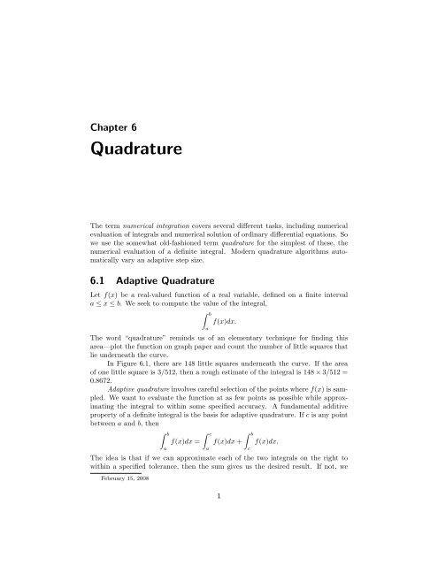
The word “quadrature” reminds us of an elementary technique for finding this 

area—plot the function on graph paper and count the number of little squares that 

lie underneath the curve. 

In Figure 6.1, there are 148 little squares underneath the curve. If the area 

of one little square is 3/512, then a rough estimate of the integral is 148 × 3/512 = 

0.8672. 

Adaptive quadrature involves careful selection of the points where f(x) is sampled. 

We want to evaluate the function at as few points as possible while approximating 

the integral to within some specified accuracy. A fundamental additive 

property of a definite integral is the basis for adaptive quadrature. If c is any point 

between a and b, then 

b c b 

f(x)dx = f(x)dx + f(x)dx. 

a 

a 

The idea is that if we can approximate each of the two integrals on the right to 

within a specified tolerance, then the sum gives us the desired result. If not, we 

February 15, 2008 

1 

c

2 Chapter 6. Quadrature 

Figure 6.1. Quadrature. 

can recursively apply the additive property to each of the intervals [a, c] and [c, b]. 

The resulting algorithm will adapt to the integrand automatically, partitioning the 

interval into subintervals with fine spacing where the integrand is varying rapidly 

and coarse spacing where the integrand is varying slowly. 

6.2 Basic Quadrature Rules 

The derivation of the quadrature rule used by our Matlab function begins with 

two of the basic quadrature rules shown in Figure 6.2: the midpoint rule and the 

trapezoid rule. Let h = b − a be the length of the interval. The midpoint rule, M, 

approximates the integral by the area of a rectangle whose base has length h and 

whose height is the value of the integrand at the midpoint: 

 

a + b 

M = hf . 

2 

The trapezoid rule, T , approximates the integral by the area of a trapezoid with 

base h and sides equal to the values of the integrand at the two endpoints: 

T = h 

f(a) + f(b) 

. 

2 

The accuracy of a quadrature rule can be predicted in part by examining its 

behavior on polynomials. The order of a quadrature rule is the degree of the lowest 

degree polynomial that the rule does not integrate exactly. If a quadrature rule of 

order p is used to integrate a smooth function over a small interval of length h, then 

a Taylor series analysis shows that the error is proportional to h p . The midpoint

6.2. Basic Quadrature Rules 3 

Midpoint rule Trapezoid rule 

Simpson’s rule Composite Simpson’s rule 

Figure 6.2. Four quadrature rules. 

rule and the trapezoid rule are both exact for constant and linear functions of x, 

but neither of them is exact for a quadratic in x, so they both have order two. (The 

order of a rectangle rule with height f(a) or f(b) instead of the midpoint is only 

one.) 

The accuracy of the two rules can be compared by examining their behavior 

on the simple integral 

1 

x 2 dx = 1 

3 . 

The midpoint rule gives 

The trapezoid rule gives 

0 

M = 1 

2 1 

= 

2 

1 

4 . 

2 0 + 1 

T = 1 

2 

= 1 

2 . 

So the error in M is 1/12, while the error in T is −1/6. The errors have opposite 

signs and, perhaps surprisingly, the midpoint rule is twice as accurate as the 

trapezoid rule.


This turns out to be true more generally. For integrating smooth functions 

over short intervals, M is roughly twice as accurate as T and the errors have opposite 

signs. Knowing these error estimates allows us to combine the two and get a rule 

that is usually more accurate than either one separately. If the error in T were 

exactly −2 times the error in M, then solving 

S − T = −2(S − M) 

for S would give us the exact value of the integral. In any case, the solution 

S = 2 1 

M + 

3 3 T 

is usually a more accurate approximation than either M or T alone. This rule 

is known as Simpson’s rule. It can also be derived by integrating the quadratic 

function that interpolates the integrand at the two endpoints, a and b, and the 

midpoint, c = (a + b)/2: 

S = h 

(f(a) + 4f(c) + f(b)). 

6 

It turns out that S also integrates cubics exactly, but not quartics, so its order 

is four. 

We can carry this process one step further using the two halves of the interval, 

[a, c] and [c, b]. Let d and e be the midpoints of these two subintervals: d = (a+c)/2 

and e = (c + b)/2. Apply Simpson’s rule to each subinterval to obtain a quadrature 

rule over [a, b]: 

S2 = h 

(f(a) + 4f(d) + 2f(c) + 4f(e) + f(b)). 

12 

This is an example of a composite quadrature rule. See Figure 6.2. 

S and S2 approximate the same integral, so their difference can be used as an 

estimate of the error: 

E = (S2 − S ). 

Moreover, the two can be combined to get an even more accurate approximation, 

Q. Both rules are of order four, but the S2 step size is half the S step size, so S2 is 

roughly 2 4 times as accurate. Thus, Q is obtained by solving 

The result is 

Q − S = 16(Q − S2). 

Q = S2 + (S2 − S )/15. 

Exercise 6.2 asks you to express Q as a weighted combination of the five function 

values f(a) through f(e) and to establish that its order is six. The rule is known 

as Weddle’s rule, the sixth-order Newton–Cotes rule, and also as the first step of 

Romberg integration. We will simply call it the extrapolated Simpson’s rule because 

it uses Simpson’s rule for two different values of h and then extrapolates toward 

h = 0.

6.3. quadtx, quadgui 5 

6.3 quadtx, quadgui 

The Matlab function quad uses the extrapolated Simpson’s rule in an adaptive 

recursive algorithm. Our textbook function quadtx is a simplified version of quad. 

The function quadgui provides a graphical demonstration of the behavior of 

quad and quadtx. It produces a dynamic plot of the function values selected by the 

adaptive algorithm. The count of function evaluations is shown in the title position 

on the plot. 

The initial portion of quadtx evaluates the integrand f(x) three times to 

give the first, unextrapolated, Simpson’s rule estimate. A recursive subfunction, 

quadtxstep, is then called to complete the computation. 

function [Q,fcount] = quadtx(F,a,b,tol,varargin) 

%QUADTX Evaluate definite integral numerically. 

% Q = QUADTX(F,A,B) approximates the integral of F(x) 

% from A to B to within a tolerance of 1.e-6. 

% 

% Q = QUADTX(F,A,B,tol) uses tol instead of 1.e-6. 

% 

% The first argument, F, is a function handle or 

% an anonymous function that defines F(x). 

% 

% Arguments beyond the first four, 

% Q = QUADTX(F,a,b,tol,p1,p2,...), are passed on to the 

% integrand, F(x,p1,p2,..). 

% 

% [Q,fcount] = QUADTX(F,...) also counts the number of 

% evaluations of F(x). 

% 

% See also QUAD, QUADL, DBLQUAD, QUADGUI. 

% Default tolerance 

if nargin < 4 | isempty(tol) 

tol = 1.e-6; 

end 

% Initialization 

c = (a + b)/2; 

fa = F(a,varargin{:}); 

fc = F(c,varargin{:}); 

fb = F(b,varargin{:}); 

% Recursive call 

[Q,k] = quadtxstep(F, a, b, tol, fa, fc, fb, varargin{:}); 

fcount = k + 3;


Each recursive call of quadtxstep combines three previously computed function 

values with two more to obtain the two Simpson’s approximations for a particular 

interval. If their difference is small enough, they are combined to return the 

extrapolated approximation for that interval. If their difference is larger than the 

tolerance, the recursion proceeds on each of the two half intervals. 

function [Q,fcount] = quadtxstep(F,a,b,tol,fa,fc,fb,varargin) 

% Recursive subfunction used by quadtx. 

h = b - a; 

c = (a + b)/2; 

fd = F((a+c)/2,varargin{:}); 

fe = F((c+b)/2,varargin{:}); 

Q1 = h/6 * (fa + 4*fc + fb); 

Q2 = h/12 * (fa + 4*fd + 2*fc + 4*fe + fb); 

if abs(Q2 - Q1)

6.4. Specifying Integrands 7 

Our textbook function does have one serious defect: there is no provision for 

failure. It is possible to try to evaluate integrals that do not exist. For example, 

1 

0 

1 

3x − 1 dx 

has a nonintegrable singularity. Attempting to evaluate this integral with quadtx 

results in a computation that runs for a long time and eventually terminates with 

an error message about the maximum recursion limit. It would be better to have 

diagnostic information about the singularity. 

6.4 Specifying Integrands 

Matlab has several different ways of specifying the function to be integrated by 

a quadrature routine. The anonymous function facility is convenient for a simple, 

one-line formula. For example, 

1 

can be computed with the statements 

f = @(x) 1./sqrt(1+x^4) 

Q = quadtx(f,0,1) 

If we want to compute π 

we could try 

f = @(x) sin(x)./x 

Q = quadtx(f,0,pi) 

0 

0 

1 

√ 1 + x 4 dx 

sin x 

x dx, 

Unfortunately, this results in a division by zero message when f(0) is evaluated 

and, eventually, a recursion limit error. One remedy is to change the lower limit of 

integration from 0 to the smallest positive floating-point number, realmin. 

Q = quadtx(f,realmin,pi) 

The error made by changing the lower limit is many orders of magnitude smaller 

than roundoff error because the integrand is bounded by one and the length of the 

omitted interval is less than 10 −300 . 

Another remedy is to use an M-file instead of an anonymous function. Create 

a file named sinc.m that contains the text 

function f = sinc(x) 

if x == 0 

f = 1; 

else 

f = sin(x)/x; 

end


Then the statement 

Q = quadtx(@sinc,0,pi) 

uses a function handle and computes the integral with no difficulty. 

Integrals that depend on parameters are encountered frequently. An example 

is the beta function, defined by 

1 

β(z, w) = 

0 

t z−1 (1 − t) w−1 dt. 

Matlab already has a beta function, but we can use this example to illustrate how 

to handle parameters. Create an anonymous function with three arguments. 

F = @(t,z,w) t^(z-1)*(1-t)^(w-1) 

Or use an M-file with a name like betaf.m. 

function f = betaf(t,z,w) 

f = t^(z-1)*(1-t)^(w-1) 

As with all functions, the order of the arguments is important. The functions used 

with quadrature routines must have the variable of integration as the first argument. 

Values for the parameters are then given as extra arguments to quadtx. To compute 

β(8/3, 10/3), you should set 

and then use 

or 

z = 8/3; 

w = 10/3; 

tol = 1.e-6; 

Q = quadtx(F,0,1,tol,z,w); 

Q = quadtx(@betaf,0,1,tol,z,w); 

The function functions in Matlab itself usually expect the first argument to 

be in vectorized form. This means, for example, that the mathematical expression 

sin x 

1 + x 2 

should be specified with Matlab array notation. 

sin(x)./(1 + x.^2) 

Without the two dots, 

sin(x)/(1 + x^2)

6.5. Performance 9 

calls for linear algebraic vector operations that are not appropriate here. The Matlab 

function vectorize transforms a scalar expression into something that can be 

used as an argument to function functions. 

Many of the function functions in Matlab require the specification of an 

interval of the x-axis. Mathematically, we have two possible notations, a ≤ x ≤ b 

or [a, b]. With Matlab, we also have two possibilities. The endpoints can be given 

as two separate arguments, a and b, or can be combined into one vector argument, 

[a,b]. The quadrature functions quad and quadl use two separate arguments. The 

zero finder, fzero, uses a single argument because either a single starting point or 

a two-element vector can specify the interval. The ordinary differential equation 

solvers that we encounter in the next chapter also use a single argument because a 

many-element vector can specify a set of points where the solution is to be evaluated. 

The easy plotting function, ezplot, accepts either one or two arguments. 

6.5 Performance 

The Matlab demos directory includes a function named humps that is intended 

to illustrate the behavior of graphics, quadrature, and zero-finding routines. The 

function is 

The statement 

h(x) = 

ezplot(@humps,0,1) 

1 

(x − 0.3) 2 + 0.01 + 

1 

(x − 0.9) 2 + 0.04 . 

produces a graph of h(x) for 0 ≤ x ≤ 1. There is a fairly strong peak near x = 0.3 

and a more modest peak near x = 0.9. 

The default problem for quadgui is 

quadgui(@humps,0,1,1.e-4) 

You can see in Figure 6.3 that with this tolerance, the adaptive algorithm has 

evaluated the integrand 93 times at points clustered near the two peaks. 

With the Symbolic Toolbox, it is possible to analytically integrate h(x). The 

statements 

syms x 

h = 1/((x-.3)^2+.01) + 1/((x-.9)^2+.04) - 6 

I = int(h) 

produce the indefinite integral 

I = 10*atan(10*x-3)+5*atan(5*x-9/2)-6*x 

The statements 

D = simple(int(h,0,1)) 

Qexact = double(D) 

produce a definite integral


100 

90 

80 

70 

60 

50 

40 

30 

20 

10 

D = 5*atan(16/13)+10*pi-6 

and its floating-point numerical value 

Qexact = 29.85832539549867 

Figure 6.3. Adaptive quadrature. 

The effort required by a quadrature routine to approximate an integral within 

a specified accuracy can be measured by counting the number of times the integrand 

is evaluated. Here is one experiment involving humps and quadtx. 

for k = 1:12 

tol = 10^(-k); 

[Q,fcount] = quadtx(@humps,0,1,tol); 

err = Q - Qexact; 

ratio = err/tol; 

fprintf(’%8.0e %21.14f %7d %13.3e %9.3f\n’, ... 

tol,Q,fcount,err,ratio) 

end 

The results are 

tol Q fcount err err/tol 

1.e-01 29.83328444174863 25 -2.504e-02 -0.250 

1.e-02 29.85791444629948 41 -4.109e-04 -0.041 

93

6.6. Integrating Discrete Data 11 

1.e-03 29.85834299237636 69 1.760e-05 0.018 

1.e-04 29.85832444437543 93 -9.511e-07 -0.010 

1.e-05 29.85832551548643 149 1.200e-07 0.012 

1.e-06 29.85832540194041 265 6.442e-09 0.006 

1.e-07 29.85832539499819 369 -5.005e-10 -0.005 

1.e-08 29.85832539552631 605 2.763e-11 0.003 

1.e-09 29.85832539549603 1061 -2.640e-12 -0.003 

1.e-10 29.85832539549890 1469 2.274e-13 0.002 

1.e-11 29.85832539549866 2429 -7.105e-15 -0.001 

1.e-12 29.85832539549867 4245 0.000e+00 0.000 

We see that as the tolerance is decreased, the number of function evaluations increases 

and the error decreases. The error is always less than the tolerance, usually 

by a considerable factor. 

6.6 Integrating Discrete Data 

So far, this chapter has been concerned with computing an approximation to the 

definite integral of a specified function. We have assumed the existence of a Matlab 

program that can evaluate the integrand at any point in a given interval. 

However, in many situations, the function is only known at a finite set of points, 

say (xk, yk), k = 1, . . . , n. Assume the x’s are sorted in increasing order, with 

a = x1 < x2 < · · · < xn = b. 

How can we approximate the integral 

b 

f(x)dx? 

a 

Since it is not possible to evaluate y = f(x) at any other points, the adaptive 

methods we have described are not applicable. 

The most obvious approach is to integrate the piecewise linear function that 

interpolates the data. This leads to the composite trapezoid rule 

n−1 

T = 

k=1 

hk 

yk+1 + yk 

, 

2 

where hk = xk+1 − xk. The trapezoid rule can be implemented by a one-liner. 

T = sum(diff(x).*(y(1:end-1)+y(2:end))/2) 

The Matlab function trapz also provides an implementation. 

An example with equally spaced x’s is shown in Figure 6.4. 

x = 1:6 

y = [6 8 11 7 5 2] 

For these data, the trapezoid rule gives


T = 35 

trapezoid 

area = 35.00 

spline 

Figure 6.4. Integrating discrete data. 

area = 35.25 

The trapezoid rule is often satisfactory in practice, and more complicated 

methods may not be necessary. Nevertheless, methods based on higher order interpolation 

can give other estimates of the integral. Whether or not they are “more 

accurate” is impossible to decide without further assumptions about the origin of 

the data. 

Recall that both the spline and pchip interpolants are based on the Hermite 

interpolation formula: 

P (x) = 3hs2 − 2s 3 

h 3 

+ s2 (s − h) 

h2 dk+1 + 

yk+1 + h3 − 3hs2 + 2s3 yk 

h3 s(s − h)2 

h2 dk, 

where xk ≤ x ≤ xk+1, s = x − xk, and h = hk. This is a cubic polynomial in s, and 

hence in x, that satisfies four interpolation conditions, two on function values and 

two on derivative values: 

P (xk) = yk, P (xk+1) = yk+1, 

P ′ (xk) = dk, P ′ (xk+1) = dk+1. 

The slopes dk are computed in splinetx or pchiptx. 

Exercise 6.20 asks you to show that 

Consequently, 

xk+1 

xk 

where T is the trapezoid rule and 

yk+1 + yk 

P (x)dx = hk − h 

2 

2 k 

b 

P (x)dx = T − D, 

a 

n−1 

D = 

k=1 

h 2 k 

dk+1 − dk 

. 

12 

dk+1 − dk 

. 

12

6.7. Further Reading 13 

The quantity D is a higher order correction to the trapezoid rule that makes use of 

the slopes computed by splinetx or pchiptx. 

If the x’s are equally spaced, most of the terms in the sum cancel each other. 

Then D becomes a simple end correction involving just the first and last slopes: 

D = h 2 dn − d1 

. 

12 

For the sample data shown in Figure 6.4, the area obtained by linear interpolation 

is 35.00 and by spline interpolation is 35.25. We haven’t shown shape-preserving 

Hermite interpolation, but its area is 35.41667. The integration process averages 

out the variation in the interpolants, so even though the three graphs might have 

rather different shapes, the resulting approximations to the integral are often quite 

close to each other. 

6.7 Further Reading 

For background on quad and quadl, see Gander and Gautschi [3]. 

Exercises 

6.1. Use quadgui to try to find the integrals of each of the following functions 

over the given interval and with the given tolerance. How many function 

evaluations are required for each problem and where are the evaluation points 

concentrated? 

f(x) a b tol 

humps(x) 0 1 10 −4 

humps(x) 0 1 10 −6 

humps(x) −1 2 10 −4 

sin x 0 π 10 −8 

cos x 0 (9/2)π 10 −6 

√ x 0 1 10 −8 

√ x log x eps 1 10 −8 

tan(sin x) − sin(tan x) 0 π 10 −8 

1/(3x − 1) 0 1 10 −4 

t 8/3 (1 − t) 10/3 0 1 10 −8 

t 25 (1 − t) 2 0 1 10 −8 

6.2. Express Q as a weighted combination of the five function values f(a) through 

f(e) and establish that its order is six. (See section 6.2.) 

6.3. The composite trapezoid rule with n equally spaced points is 

Tn(f ) = h 

2 

n−2 

f(a) + h 

k=1 

f(a + kh) + h 

2 f(b),


where 

b − a 

h = 

n − 1 . 

Use Tn(f ) with various values of n to compute π by approximating 

1 

π = 

−1 

2 

dx. 

1 + x2 How does the accuracy vary with n? 

6.4. Use quadtx with various tolerances to compute π by approximating 

1 

π = 

−1 

2 

dx. 

1 + x2 How do the accuracy and the function evaluation count vary with tolerance? 

6.5. Use the Symbolic Toolbox to find the exact value of 

1 

0 

x4 (1 − x) 4 

1 + x2 dx. 

(a) What famous approximation does this integral bring to mind? 

(b) Does numerical evaluation of this integral present any difficulties? 

6.6. The error function erf(x) is defined by an integral: 

erf(x) = 2 

√ π 

x 

0 

e −x2 

dx. 

Use quadtx to tabulate erf(x) for x = 0.1, 0.2, . . . , 1.0. Compare the results 

with the built-in Matlab function erf(x). 

6.7. The beta function, β(z, w), is defined by an integral: 

1 

β(z, w) = 

0 

t z−1 (1 − t) w−1 dt. 

Write an M-file mybeta that uses quadtx to compute β(z, w). Compare your 

function with the built-in Matlab function beta(z,w). 

6.8. The gamma function, Γ(x), is defined by an integral: 

∞ 

Γ(x) = 

0 

t x−1 e −t dt. 

Trying to compute Γ(x) by evaluating this integral with numerical quadrature 

can be both inefficient and unreliable. The difficulties are caused by the 

infinite interval and the wide variation of values of the integrand. 

Write an M-file mygamma that tries to use quadtx to compute Γ(x). Compare 

your function with the built-in Matlab function gamma(x). For what x is 

your function reasonably fast and accurate? For what x does your function 

become slow or unreliable?

Exercises 15 

6.9. (a) What is the exact value of 

4π 

cos 2 x dx? 

(b) What does quadtx compute for this integral? Why is it wrong? 

(c) How does quad overcome the difficulty? 

6.10. (a) Use ezplot to plot x sin 1 

x for 0 ≤ x ≤ 1. 

(b) Use the Symbolic Toolbox to find the exact value of 

1 

x sin 1 

x dx. 

(c) What happens if you try 

quadtx(@(x) x*sin(1/x),0,1) 

0 

0 

(d) How can you overcome this difficulty? 

6.11. (a) Use ezplot to plot xx for 0 ≤ x ≤ 1. 

(b) What happens if you try to use the Symbolic Toolbox to find an analytic 

expression for 

1 

x x dx? 

0 

(c) Try to find the numerical value of this integral as accurately as you can. 

(d) What do you think is the error in the answer you have given? 

6.12. Let 

f(x) = log(1 + x) log(1 − x). 

(a) Use ezplot to plot f(x) for −1 ≤ x ≤ 1. 

(b) Use the Symbolic Toolbox to find an analytic expression for 

1 

f(x)dx. 

(c) Find the numerical value of the analytic expression from (b). 

(d) What happens if you try to find the integral numerically with 

−1 

quadtx(@(x)log(1+x)*log(1-x),-1,1) 

(e) How do you work around this difficulty? Justify your solution. 

(f ) Use quadtx and your workaround with various tolerances. Plot error 

versus tolerance. Plot function evaluation count versus tolerance. 


f(x) = x 10 − 10x 8 + 33x 6 − 40x 4 + 16x 2 . 

(a) Use ezplot to plot f(x) for −2 ≤ x ≤ 2. 

(b) Use the Symbolic Toolbox to find an analytic expression for 

2 

f(x)dx. 

−2


(c) Find the numerical value of the analytic expression. 

(d) What happens if you try to find the integral numerically with 

F = @(x) x^10-10*x^8+33*x^6-40*x^4+16*x^2 

quadtx(F,-2,2) 

Why? 

(e) How do you work around this difficulty? 

6.14. (a) Use quadtx to evaluate 

2 

−1 

1 

sin( |t|) dt. 

(b) Why don’t you encounter division-by-zero difficulties at t = 0? 

6.15. Definite integrals sometimes have the property that the integrand becomes 

infinite at one or both of the endpoints, but the integral itself is finite. In 

other words, limx→a |f(x)| = ∞ or limx→b |f(x)| = ∞, but 

b 

f(x) dx 

a 

exists and is finite. 

(a) Modify quadtx so that, if an infinite value of f(a) or f(b) is detected, 

an appropriate warning message is displayed and f(x) is reevaluated at a 

point very near to a or b. This allows the adaptive algorithm to proceed and 

possibly converge. (You might want to see how quad does this.) 

(b) Find an example that triggers the warning, but has a finite integral. 

6.16. (a) Modify quadtx so that the recursion is terminated and an appropriate 

warning message is displayed whenever the function evaluation count exceeds 

10,000. Make sure that the warning message is only displayed once. 

(b) Find an example that triggers the warning. 

6.17. The Matlab function quadl uses adaptive quadrature based on methods 

that have higher order than Simpson’s method. As a result, for integrating 

smooth functions, quadl requires fewer function evaluations to obtain a specified 

accuracy. The “l” in the function name comes from Lobatto quadrature, 

which uses unequal spacing to obtain higher order. The Lobatto rule used in 

quadl is of the form 

1 

f(x) dx = w1f(−1) + w2f(−x1) + w2f(x1) + w1f(1). 

−1 

The symmetry in this formula makes it exact for monic polynomials of odd 

degree f(x) = x p , p = 1, 3, 5, . . . . Requiring the formula to be exact for 

even degrees x 0 , x 2 , and x 4 leads to three nonlinear equations in the three 

parameters w1, w2, and x1. In addition to this basic Lobatto rule, quadl 

employs even higher order Kronrod rules, involving other abscissae, xk, and 

weights, wk.

Exercises 17 

(a) Derive and solve the equations for the Lobatto parameters w1, w2, and 

x1. 

(b) Find where these values occur in quadl.m. 


1 

Ek = x k e x−1 dx. 

(a) Show that 

and that 

0 

E0 = 1 − 1/e 

Ek = 1 − kEk−1. 

(b) Suppose we want to compute E1, . . . , En for n = 20. Which of the 

following approaches is the fastest and most accurate? 

• For each k, use quadtx to evaluate Ek numerically. 

• Use forward recursion: 

E0 = 1 − 1/e; 

for k = 2, . . . , n, Ek = 1 − kEk−1. 

• Use backward recursion, starting at N = 32 with a completely inaccurate 

value for EN : 

EN = 0; 

for k = N, . . . , 2, Ek−1 = (1 − Ek)/k; 

ignore En+1, . . . , EN. 

6.19. An article by Prof. Nick Trefethen of Oxford University in the January/February 

2002 issue of SIAM News is titled “A Hundred-dollar, Hundred-digit Challenge” 

[2]. Trefethen’s challenge consists of ten computational problems, each 

of whose answers is a single real number. He asked for each answer to be computed 

to ten significant digits and offered a $100 prize to the person or group 

who managed to calculate the greatest number of correct digits. Ninety-four 

teams from 25 countries entered the computation. Much to Trefethen’s surprise, 

20 teams scored a perfect 100 points and five more teams scored 99 

points. A follow-up book has recently been published [1]. 

Trefethen’s first problem is to find the value of 

1 

T = lim x 

ɛ→0 

−1 cos (x −1 log x) dx. 

ɛ 

(a) Why can’t we simply use one of the Matlab numerical quadrature routines 

to compute this integral with just a few lines of code? 

Here is one way to compute T to several significant digits. Express the 

integral as an infinite sum of integrals over intervals where the integrand 

does not change sign: 

∞ 

T = Tk, 

k=1


where 

xk−1 

Tk = 

xk 

x −1 cos (x −1 log x)dx. 

Here x0 = 1, and, for k > 0, the xk’s are the successive zeros of cos (x −1 log x), 

ordered in decreasing order, x1 > x2 > · · · . In other words, for k > 0, xk 

solves the equation 

log xk 

xk 

 

= − k − 1 

 

π. 

2 

You can use a zero finder such as fzerotx or fzero to compute the xk’s. 

If you have access to the Symbolic Toolbox, you can also use lambertw to 

compute the xk’s. For each xk, Tk can be computed by numerical quadrature 

with quadtx, quad, or quadl. The Tk’s are alternately positive and negative, 

and hence the partial sums of the series are alternately greater than and less 

than the infinite sum. Moreover, the average of two successive partial sums 

is a more accurate approximation to the final result than either sum by itself. 

(b) Use this approach to compute T as accurately as you can with a reasonable 

amount of computer time. Try to get at least four or five digits. You may be 

able to get more. In any case, indicate how accurate you think your result is. 

(c) Investigate the use of Aitken’s δ 2 acceleration 

(Tk+1 − Tk) 2 

˜Tk = Tk − 

. 

Tk+1 − 2Tk + Tk−1 

6.20. Show that the integral of the Hermite interpolating polynomial 

P (s) = 3hs2 − 2s 3 

h 3 

+ s2 (s − h) 

h2 dk+1 + 

over one subinterval is 

h 

P (s)ds = h yk+1 + yk 

2 

0 

yk+1 + h3 − 3hs2 + 2s3 yk 

h 3 

s(s − h)2 

h2 dk 

− h 2 dk+1 − dk 

. 

12 

6.21. (a) Modify splinetx and pchiptx to create splinequad and pchipquad that 

integrate discrete data using spline and pchip interpolation. 

(b) Use your programs, as well as trapz, to integrate the discrete data set 

x = 1:6 

y = [6 8 11 7 5 2] 

(c) Use your programs, as well as trapz, to approximate the integral 

1 

0 

4 

dx. 

1 + x2 Generate random discrete data sets using the statements

Exercises 19 

x = round(100*[0 sort(rand(1,6)) 1])/100 

y = round(400./(1+x.^2))/100 

With infinitely many infinitely accurate points, the integrals would all equal 

π. But these data sets have only eight points, rounded to only two decimal 

digits of accuracy. 

6.22. This program uses functions in the Spline Toolbox. What does it do? 

x = 1:6 

y = [6 8 11 7 5 2] 

for e = [’c’,’n’,’p’,’s’,’v’] 

disp(e) 

ppval(fnint(csape(x,y,e)),x(end)) 

end 

6.23. How large is your hand? Figure 6.5 shows three different approaches to 

computing the area enclosed by the data that you obtained for exercise 3.3. 

Q = 0.3991 Q = 0.4075 Q = 0.4141 

Figure 6.5. The area of a hand. 

(a) Area of a polygon. Connect successive data points with straight lines and 

connect the last data point to the first. If none of these lines intersect, the 

result is a polygon with n vertices, (xi, yi). A classic, but little known, fact 

is that the area of this polygon is 

(x1y2 − x2y1 + x2y3 − x3y2 + · · · + xny1 − x1yn)/2. 

If x and y are column vectors, this can be computed with the Matlab oneliner 

(x’*y([2:n 1]) - x([2:n 1])’*y)/2 

(b) Simple quadrature. The Matlab function inpolygon determines which 

of a set of points is contained in a given polygonal region in the plane. The 

polygon is specified by the two arrays x and y containing the coordinates of 

the vertices. The set of points can be a two-dimensional square grid with 

spacing h. 

[u,v] = meshgrid(xmin:h:xmax,ymin:h:ymax)


The statement 

k = inpolygon(u,v,x,y) 

returns an array the same size as u and v whose elements are one for the 

points in the polygon and zero for the points outside. The total number of 

points in the region is the number of nonzeros in k, that is, nnz(k), so the 

area of the corresponding portion of the grid is 

h^2*nnz(k) 

(c) Two-dimensional adaptive quadrature. The characteristic function of the 

region χ(u, v) is equal to one for points (u, v) in the region and zero for points 

outside. The area of the region is 

 

χ(u, v)dudv. 

The Matlab function inpolygon(u,v,x,y) computes the characteristic function 

if u and v are scalars, or arrays of the same size. But the quadrature 

functions have one of them a scalar and the other an array. So we need an 

M-file, chi.m, containing 

function k = chi(u,v,x,y) 

if all(size(u) == 1), u = u(ones(size(v))); end 

if all(size(v) == 1), v = v(ones(size(u))); end 

k = inpolygon(u,v,x,y); 

Two-dimensional adaptive numerical quadrature is obtained with 

dblquad(@chi,xmin,xmax,ymin,ymax,tol,[],x,y) 

This is the least efficient of the three methods. Adaptive quadrature expects 

the integrand to be reasonably smooth, but χ(u, v) is certainly not smooth. 

Consequently, values of tol smaller than 10 −4 or 10 −5 require a lot of computer 

time. 

Figure 6.5 shows that the estimates of the area obtained by these three methods 

agree to about two digits, even with fairly large grid sizes and tolerances. 

Experiment with your own data, use a moderate amount of computer time, 

and see how close the three estimates can be to each other.

Bibliography 

[1] F. Bornemann, D. Laurie, S. Wagon, and J. Waldvogel, The SIAM 

100-Digit Challenge: A Study in High-Accuracy Numerical Computing, SIAM, 

Philadelphia, 2004. 

[2] L. N. Trefethen, A hundred-dollar, hundred-digit challenge, SIAM News, 

35(1)(2002). Society of Industrial and Applied Mathematics. 

http://www.siam.org/pdf/news/388.pdf 

http://www.siam.org/books/100digitchallenge 

[3] W. Gander and W. Gautschi, Adaptive Quadrature—Revisited, BIT Numerical 

Mathematics, 40 (2000), pp. 84–101. 

http://www.inf.ethz.ch/personal/gander 

21

Chapter 6. Quadrature - MathWorks

Create successful ePaper yourself

Delete template?

Save as template?