Forecasting GDP with a Dynamic Factor Model - MathWorks
Forecasting GDP with a Dynamic Factor Model - MathWorks
Forecasting GDP with a Dynamic Factor Model - MathWorks

Create successful ePaper yourself
Turn your PDF publications into a flip-book with our unique Google optimized e-Paper software.
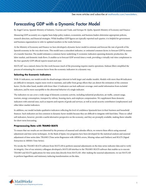
<strong>Forecasting</strong> <strong>GDP</strong> <strong>with</strong> a <strong>Dynamic</strong> <strong>Factor</strong> <strong>Model</strong><br />
By Ángel Cuevas, Spanish Ministry of Industry, Tourism and Trade, and Enrique M. Quilis, Spanish Ministry of Economy and Finance<br />
Measuring <strong>GDP</strong> accurately on a regular basis helps policy makers, economists, and business leaders determine appropriate policies,<br />
research direction, and financial strategies. While headline <strong>GDP</strong> figures are typically reported each quarter, it is helpful for government<br />
and business organizations to refer to updated numbers in the weeks between.<br />
At the Ministry of Economy and Finance we have developed a dynamic factor model to estimate and forecast the rate of growth of the<br />
Spanish economy in the very short term. This model uses a coincident indicator, or estimated common factor, to forecast <strong>GDP</strong> by means<br />
of a transfer function. The model estimates a common factor underlying 31 economic indicators spanning domestic production, the<br />
labor market, and domestic trade flows. It enables us to forecast <strong>GDP</strong> several times a week, providing a virtually real-time complement to<br />
the four quarterly <strong>GDP</strong> official reports issued each year.<br />
MATLAB ® was a natural choice for this work because much of the processing requires matrix operations. Kalman filters simplified the<br />
process of estimating the common factor from the economic indicators in a dynamic way.<br />
Selecting the Economic Indicators<br />
With 31 indicators, our model avoids the disadvantages inherent in both larger and smaller models. <strong>Model</strong>s <strong>with</strong> more than 80 indicators<br />
are difficult to interpret, require more work to maintain, and suffer from group effects that can distort the estimation of the common<br />
factor. On the other hand, models <strong>with</strong> fewer than 12 indicators can lack sufficient coverage, omit useful information from excluded<br />
indicators, and be more susceptible to the abnormal behavior of a single indicator.<br />
The indicators we use cover a wide range of domestic economic activity, including industrial production, air traffic, cement usage,<br />
tourism, energy consumption, transport by railway, housing starts, and employee compensation. We supplement these domestic<br />
indicators <strong>with</strong> external ones, such as imports and exports of goods and services, as well as social security contributors (employment) and<br />
other labor-market indicators.<br />
In addition, our model includes qualitative indicators reflecting the level of confidence Spaniards have in their business and household<br />
finances. Such indicators are less common in dynamic factor models because they are difficult to integrate <strong>with</strong> hard data. These so-called<br />
soft indicators, however, provide a useful alternative perspective on the economy, and they are promptly available, making them valuable<br />
for short-term forecasting.<br />
Preprocessing Data <strong>with</strong> TRAMO-SEATS<br />
To ensure that our results are not distorted by the presence of seasonal and calendar effects, we remove these effects using seasonal<br />
adjustment and time series techniques. At the Bank of Spain, two programs have been developed for the statistical analysis and seasonal<br />
adjustment of time series data: TRAMO (Time series Regression <strong>with</strong> ARIMA errors, Missing values and Outliers) and SEATS (Signal<br />
Extraction in ARIMA Time Series).<br />
We invoke the TRAMO-SEATS software from MATLAB to perform seasonal adjustments on the time series indicator data and to verify<br />
its integrity. One of our ministry colleagues developed a MATLAB interface to the TRAMO-SEATS software that enables us to execute<br />
TRAMO and SEATS applications for time series data directly from MATLAB. After making the seasonal adjustments, we use MATLAB<br />
to perform logarithmic and stationary-inducing transformation on the data.<br />
See more articles and subscribe at mathworks.com/newsletters.<br />
1
Developing the <strong>Dynamic</strong> Common <strong>Factor</strong> <strong>Model</strong><br />
The common factor model must consider both static and dynamic interactions among the observed indicators. We use MATLAB to<br />
estimate the common factor <strong>with</strong> principal components. We then use a Kalman filter to introduce dynamics into the model. A complete<br />
representation of the dynamic factor model implemented in MATLAB has the form<br />
where Zt are observations, ft is the common factor, Ut are idiosyncratic factors, L is a factor loading matrix, Φf(B) is an AR(4) operator,<br />
ΦU(B) is a VAR(1) operator <strong>with</strong> diagonal AR(1) matrix, Qe is a diagonal matrix, and B is the lag (or backshift) operator BZt = Zt-1.<br />
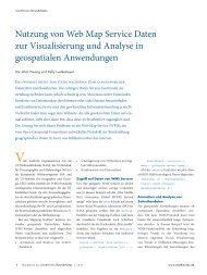
Among the biggest operational challenges that we faced in developing the model was analyzing data from different time periods. We had<br />
a complete set of observed data for several indicators over the entire time period (a longitudinal panel), as well as observed data for all<br />
indicators over a shorter time period (a cross-section panel). What we lacked was a complete set of observed data for all indicators over<br />
the entire time period (Figure 1).<br />
Figure 1. An unbalanced panel, <strong>with</strong> missing data for some indicators.<br />
To handle this unbalanced panel, we implemented an iterative process in MATLAB that begins <strong>with</strong> the estimation of a static factor<br />
model by principal components using the longitudinal panel data. Indicators that were excluded from the longitudinal panel are<br />
individually regressed using ordinary least squares. We then calculate a new factor from the statically balanced panel and apply a Kalman<br />
filter to estimate the missing values. This process, which is repeated until convergence is achieved, is based on an approach outlined by<br />
Chang-Jin Kim and Charles R. Nelson [1].<br />
2
Generating the <strong>GDP</strong> Forecast<br />
After estimating the common factor using the dynamic factor model, we use a transfer function model to forecast <strong>GDP</strong>. This model<br />
defines a simple and quantitatively consistent relationship between the common factor and the <strong>GDP</strong> or other macroeconomic aggregates.<br />
We use a time series analysis package to derive the parameters of the transfer function and then implement it using MATLAB. We check<br />
the specification of the transfer function <strong>with</strong> the results of a bivariate vector autoregressive and moving average (VARMA) model.<br />
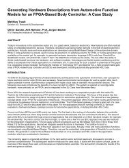
Finally, we use the MATLAB filter function to forecast the current quarter <strong>GDP</strong> based on the common factor and the transfer<br />
function. Figure 2 shows the relation of the estimated factor and the <strong>GDP</strong> quarter-on-quarter rate of growth.<br />
Figure 2. Temporal aggregation of the common factor (red) and <strong>GDP</strong> (blue) from 1990 to 2010.<br />
We update the <strong>GDP</strong> forecasts whenever we have new data for one of our indicators, which can be several times a week. MATLAB<br />
completes all the calculations in minutes, enabling us to deliver results almost in real time. We produce our reports by exporting our data<br />
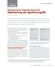
from the MATLAB workspace into a Microsoft ® Excel ® spreadsheet using Spreadsheet Link EX. Since the common factor is closely<br />
linked to <strong>GDP</strong> growth and can be computed in a more timely fashion, it provides economists and business leaders <strong>with</strong> a reasonably<br />
accurate estimate of Spain’s <strong>GDP</strong> well before the official <strong>GDP</strong> numbers are released (Figure 3).<br />
Figure 3. Real-time forecasts (plus ±σ interval) and final <strong>GDP</strong> data.<br />
3
Cyclical Analysis<br />
In addition to <strong>GDP</strong> forecasting, we use the dynamic factor model in other economic studies, including the simulation of macro scenarios<br />
and cyclical analysis. For example, we have used the model and cyclical bandpass filters to identify turning points in the business cycle for<br />
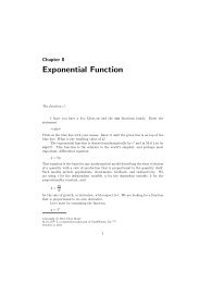
the past 20 years. Using Signal Processing Toolbox, we applied a Butterworth filter to extract the signal from the data and pinpoint<br />
cyclical turning points (Figure 4). We use a bandpass Butterworth filter because it provides a cleaner picture of economic fluctuations<br />
than the Hodrick-Prescott filter, which acts like an implicit high-pass filter that leaks high-frequency noise. The absence of irregular<br />
components makes it considerably easier for the algorithms to identify business cycle turning points.<br />
Figure 4. Business cycle turning points in the Spanish economy, 1990-2010, identified using a MATLAB based dynamic factor model. Turning<br />
points play a qualitative role, defining business cycle phases: expansions (from trough to peak) and recessions (from peak to trough).<br />
We continue to refine the estimation procedures in the model <strong>with</strong> MATLAB, and we update the list of indicators as needed to improve<br />
the accuracy of our forecasts.<br />
Reference<br />
[1] Chang-Jin Kim and Charles R. Nelson, State-Space <strong>Model</strong>s <strong>with</strong> Regime Switching, MIT Press 1999.<br />
Products Used<br />
▪ MATLAB<br />
▪ Signal Processing Toolbox<br />
▪ Spreadsheet Link EX<br />
mathworks.com<br />
Learn More<br />
▪ A <strong>Factor</strong> Analysis for the Spanish Economy<br />
▪ Download: MATLAB interface for TRAMO-SEATS<br />
See more articles and subscribe at mathworks.com/newsletters.<br />
© 2012 The <strong>MathWorks</strong>, Inc. MATLAB and Simulink are registered trademarks of The <strong>MathWorks</strong>, Inc. See www.mathworks.com/trademarks<br />
for a list of additional trademarks. Other product or brand names may be trademarks or registered trademarks of their respective holders.<br />
Published 2012<br />
92011v00<br />
4