Assessment of the Automation Algorithm for TDR Bridge - Ohio ...

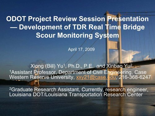
ODOT Project Review Session Presentation
— Development of TDR Real Time Bridge
Scour Monitoring System
April 17, 2009
Xiong (Bill) Yu 1 , Ph.D., P.E. and Xinbao Yu 2
1 Assistant Professor, Department of Civil Engineering, Case
Western Reserve University, xxy21@case.edu, 216-368-6247
2 Graduate Research Assistant, Currently, research engineer,
Louisiana DOT/Louisiana Transportation Research Center

Outline
• Introduction
• Literature review: scour monitoring
practice and technologies
• Validation of Time Domain Reflectometry
for scour monitoring
• TDR scour measurements in various
environments
• Development of a field TDR scour sensor
• Summary and conclusions, and future
work
2

Introduction
1.1 Motivation for Bridge Scour Monitoring
• 1987, the Schoharie Creek Bridge on the New York State Thruway
• 1989, the US 51 bridge over the Hatchie River in Tennessee
• 1995, the I-5 bridges over Arroyo Pasajero in California
National Bridge
Inspection
Standards (NBIS)
Minimum 2 year
inspection
frequency
3

1.2 Fundamentals of Bridge Scour
• Definition
• A dynamic process
Pier scour depth in a sand-bed stream as a function of time (Richardson 1995)
4

Classification
• General Scour
• Aggradation and Degradation
• Contraction Scour
• Local Scour
Different Types of Scour in a Typical Bridge Cross Section (Wang 2004).
5

Contraction scour
Two manmade features that create a contracted
section in a channel (Sheppard and Renna 2005)
An example of manmade causeway islands that create a
channel contraction (Sheppard and Renna 2005)
6

Local Scour
• Pier scour and abutment scour
Scour design references
Complex flows around a bridge pier (Hamill 1999)
HEC-18, Evaluating Scour at Bridges
HEC-20, Stream Stability at Highway Bridges
HEC-23, Bridge Scour and Stream Instability
Countermeasures-Experience, Selection, and Design Guidance
7

1.3 Bridge Scour Study
• Analytical Methods
Vortex, scour depth, assumption of the scour shape, determination of
critical shear stress or critical velocity, and continuity equation
• Physical Modeling
• Numerical Simulation
Photo of a pier scour flume test
8

Physical Modeling
Parameters related to fluid properties
• g: acceleration due to gravity
• ρ: density of the fluid
• υ: kinematic viscosity of fluid
Parameters related to flow properties
• y1 : approach flow depth
d
• V1: approach mean flow velocity
s
Parameters related to sediment properties b
• ρ: density of the sediment
• d50 : median sediment size
• σg: geometric standard deviation of sediment size
distribution
• cohesion of sediment
Parameters related to the bridge pier
• shape of the bridge pier
• width of the bridge pier
• alignment of the bridge pier
Breusers et al. 1997
⎛
⎞
⎜
y1
V1
ρV1b
V1
b
= f K
⎟
s,
Kθ
, , , , , , σ g
⎜
⎟
⎝
b gy µ Vc
d
1
50 ⎠
9

Numerical Simulation
• 1D simulation such as HEC-RAS and WSPRO
• 2D simulation such as Flo2dh and SED2D
• 3D simulation such as Flow3D, FLUENT, and CCHE3D
Screen shot of bridge
scour analysis in HEC-
RAS
Example of flow field by
Flo2dh (Yu and Yu 2008)
10

Numerical Simulation
• 1D simulation such as HEC-RAS and WSPRO
• 2D simulation such as Flo2dh and SED2D
• 3D simulation such as Flow3D, FLUENT, and CCHE3D
Simulated local scour hole around
a bridge pier (NCCHE n.d.)
Simulated complex turbulent flow around
bridge piers (Ge 2004)
11

Numerical Simulation
• 3D simulation such as Flow3D, FLUENT, and CCHE3D
turbulent flow
two-phase flow: air, water, sediment
fluid sediment interaction
According to the previous research, it
is found that the bottleneck of the
state-of-the-art of the local scour
simulation lies in the accurate
modeling of the sediment behavior and
the interaction between the flow and
bed variation.
12

Field observation
• A co-operative National Bridge Scour Project in 1987 to collect
scour data at bridges during floods by USGS and FHWA
• The second USGS field-collection funded by FHWA (2005)
Muller and Wagner (2005) … a deficiency that is primarily a reflection of the difficulty in
collecting the necessary data. Accurate and complete field measurements of scour are
difficult to obtain because of complex hydraulic conditions at bridges during floods, inability
to get skilled personnel to bridge sites during floods, and problems associated with existing
measuring equipment.
13

Outline
• Introduction
• Literature review: scour monitoring
practice and technologies
• Validation of Time Domain Reflectometry
for scour monitoring
• TDR scour measurements in various
environments
• Development of a field TDR scour sensor
• Summary and conclusions, and future
work
14

Literature review: scour monitoring
practice and technologies
• Fixed instruments
• Portable instruments
• Visual inspection
15

2.1 Motivation for Scour Instrumentation
• Hunt (2005)
safety for the traveling public
a reduced number of underwater and/or regular
inspections
early identification of problems prior to a diving inspection
insight into site-specific scour processes
Hawaii DOT, validation of HEC-18 equations by sonar
devices
Good instrumentation is essential for making proper
decision, Georgia 1994 flood, 1000 bridge closed
16

2.1 Motivation for Scour Instrumentation
(cont.)
• Challenges for scour monitoring instrumentations
• Criteria for the instrumentation
Mandatory Criteria
•Capability for installation on or near a bridge pier
or abutment
•Ability to measure maximum scour depth within
an accuracy of 0.3 m (1 ft)
•Ability to obtain scour depth readings from above
the water or from a remote site
•Operable during storm and flood conditions
Site conditions that cause
interference or damage to
the fixed scour monitoring
systems (Hunt 2005)
Desirable Criteria
•Capability to be installed on most existing
bridges or during construction of new bridges
•Capability to operate in a range of flow
conditions
•Capability to withstand ice and debris
•Vandal resistant
•Operable and maintainable by highway
maintenance personnel
17

2.2 National Practice of Developing
Instrumentation for Scour Monitoring
• Zabilansky, 1996
White River Junction, Vermont
Instrumented fish and sediment chains
(Zabilansky 1996)
18

• Lagasse and Price 1997
NCHRP Project 21-3, Instrumentation for
Measuring Scour at Bridge Piers and Abutments
1. Sounding rods: manual or mechanical device
(rod) to probe streambed;
2. Buried or driven rods: device with sensors on
vertical support, place or driven to streambed;
3. Fathometers: commercially available sonic finder;
and
4. Other buried devices: active or inert buried sensor
(e.g., buried transmitter).
Products: Sonic fathometers and a magnetic sliding
collar device
19

• Mueller and Landers 1999
development of portable instruments for bridge
scour monitoring
1. physical probing such as sounding poles
and sounding weights;
2. sonar such as single-beam sonar, side
scan, multi-beam, and scanning sonar;
3. geophysical such as seismic instruments;
4. and other such as underwater camera
and green laser sensor
Products: a low-cost echo sounder and a
tethered kneeboard to deploy the transducer
20

• Mueller and Landers 1999
PVC-pontoon float for deploying a
transducer
A remote-control boat being
tested near a pier
21

• Schall and Price 2004
NCHRP Project 21-07, portable scour instruments
Products
a portable scour monitoring device
a fully instrumented articulated arm truck
Articulated arm truck making a scour
measurement (Schall and Price 2004)
22

National practice of scour monitoring
• Hunt 2005, a synthesis study
Total number of bridge sites with
fixed scour monitoring
instrumentation
States with fixed scour monitoring
installations
23

2.3 Technologies for Scour Monitoring
• Sonar
• Magnetic Sliding Collar (MSC)
• Time Domain Reflectometry (TDR)
Sonar
SOund NAvigation and Ranging
active and passive
echo sounders, fathometers, and acoustic depth sounders
•Theory
V (in feet per second) = 4388+
(11.25 temperature (in F)) + (0.0182
depth (in feet)) + salinity (in parts-perthousand)
24

Sonar (cont.)
A sonar system for bridge scour
monitoring (Nassif et al. 2002)
Schematic of a sonar scour monitoring
system over Fire Island Inlet (Hunt 2005)
25

Sonar (cont.)
• wave frequency
200 kHz
• beam width Illustration of transducer beamwidth
(Muller and Landers 1999)
Effect of beamwidth on measured depth
(Muller and Landers 1999)
26

Sonar (cont.)
• Data Acquisition
• Limitations
Fathometer data recorded with 200 kHz
transducer (fathometer n.d.)
1. at least 3 m and velocities less than 4 m/s
2. turbulence, air entrainment, and heavy suspendedsediment
3. noise from multiple reflections, and echoes from the
shoreline, water bottom, and/or piers
27

Magnetic Sliding Collar
• NCHRP Project 21-3 by Lagasse and Price (1997)
• Basic Concepts
A sliding magnetic collar on stainless steel
pipe with driving point (Cooper et al. 2000).
Schematic plot of magnetic sliding collar
(Fukui and Otuka n.d.)
• Limitations: shallow stream, refill, accuracy
28

Time Domain Reflectometry
Dowding and Pierce (1994)
Yankielun and Zabilansky
(1999)
29

Basics
Concepts
EM Wave
v
p
=
c
µ ε
A TDR system
r
r
A schematic plot of a TDR system
Relative Voltage (V)
1.25
0.75
0.25
-0.25
-0.75
K
a
⎛
= ⎜
L
= ⎜
L
=
⎜
⎝ L
a
p
⎞
⎟
⎟
⎠
V s/2
2
Apparent Length, L a
-1.25
0 1 2 3 4 5 6 7 8
Scaled Distance (m)
A TDR waveform
EC
b
1 ⎛ ⎞
⎜
V ⎞
= ⎜
V ⎞ s
= ⎜
V s
= − 1 ⎟
C ⎜ ⎟
⎝V
⎟
⎝V
⎟
⎝V
f ⎠
V f
30

Reflection at Interface
Reflection coefficient
ρ =
Air, Ka=1
Z
Z
2
2
−
+
Z
Z
1
1
=
K
K
a,
1
a,
1
−
+
K
K
a,
2
a,
2
Saturated soil, Ka=20~40 depending on density
Water, Ka=81
Change of impedance will cause
reflection of EM wave
Air
Water
Sediment
TDR sensor for Bridge scour
monitoring

Signal Analysis
Topp et al. (1982)
Baker and Allmaras (1990)
32

Outline
• Introduction
• Literature review: scour monitoring
practice and technologies
• Validation of Time Domain Reflectometry
for scour monitoring
• TDR scour measurements in various
environments
• Development of a field TDR scour sensor
• Summary and conclusions, and future
work
33

Validation of Time Domain Reflectometry
for Scour Monitoring
• TDR Measurements of Simulated Scour in laboratory
• Algorithms for TDR Signal Interpretation
Sediment
Photo of fine sand
100%
80%
60%
40%
20%
0%
1.00
Grain diameter (mm)
0.10
0.01
Grain size distribution of fine sand
% passing
34

Experiment Setup and Procedure
• Sand deposit gradually added while maintaining a
constant water level
• At each stage, a TDR signal is obtained

Data acquisition
36

Voltage(V)
Test results
0.4
0.0
-0.4
-0.8
-1.2
Increase of thickness of sediments
thickness of sediments: 16cm
thickness of sediments: 12cm
thickness of sediments: 8cm
thickness of sediments: 4cm
thickness of sediments: 0cm
0 2 4
Length(m)
6 8
Increment Thickness (cm) K a,m EC b,m
Sand
added
Sand Water mS/m g
1 0 24 87.27 23.25 0
2 4 20 74.43 20.982 3542
3 8 16 62.92 17.953 3195
4 12.5 11.5 50.01 14.82 3915
5 16 8 44.85 13.593 3220
6 20.5 3.5 31.62 10.394 3540
7 21.7 2.3 32 9.578 990
8 23.5 0.5 28.87 8.374 1731
TDR waveforms for different scour depth 37

Test results (cont.)
K a,m
K a,m
90
80
70
60
50
40
30
20
100
80
60
40
20
0
y = -2.4799x + 84.418
R² = 0.9891
0 5 10 15 20 25
Thickness of Sediment Layer(cm)
Fine sand in tap water
Fine sand in 250ppm NaCl solution
Fine sand in 500ppm NaCl solution
Fine sand in 750ppm NaCl solution
0 5 10 15 20 25 30 35
Thickness of sand layer (cm)
EC b,m(mS/m)
25
20
15
10
Saline water
EC b,m
Tap water
120
110
100
90
80
70
60
50
40
30
20
10
5
0
y = -0.6294x + 23.224
R² = 0.997
0 5 10 15 20 25
Thickness of Sediment Layer(cm)
Fine sand in tap water
Fine sand in 250ppm NaCl solution
Fine sand in 500ppm NaCl solution
Fine sand in 750ppm NaCl solution
0 5 10 15 20 25 30 35
Thickness of sand layer (cm)
38

3.2 Algorithms for TDR Signal Interpretation
• Dielectric mixing formula for scour estimation
n
α ( K ) = υ ( K )
a,
m
∑
i=
1
i
a,
i
L 1 Ka,
w + L2
Ka,
bs = L Ka,
m
K
K
a,
m
a,
w
=
x
L
⎛
⎜
⎜
⎝
K
K
a,
bs
a,
w
α
⎞
−1⎟
+ 1
⎟
⎠
(Birchak et al. 1974)
Water L1
Sediment L2
Setting the thickness of sediment L2 equal to x
Dielectric scour estimation equation
Approximate linear relationship between √K a,m and
sediment thickness
Sediment thickness can be estimated from measured K a,m
39

Mixing Formula for Dielectric Constant and
its Application
Measured and
predicted √K a,m /√K a,w
versus sediment
thickness
Estimated thickness of sand layer (cm)
30
25
20
15
10
5
0
Fine sand in tap water
Fine sand in 250ppm solution
Linear Fit of Estimated thickness of sand layer
Equation
Weight
Residual Sum
of Squares
Adj. R-Square
Estimated
thickness of
sand layer
y = a + b*x
No Weighting
2.3419
0.99859
0 5 10 15 20 25 30 35
Measured thickness of sand layer (cm)
Value Standard Error
Intercept 0 --
Slope 0.98828 0.01315
Thickness of sand layer estimated by the
dielectric constant mixing formula
40

Mixing Formula for Electrical Conductivity and
its Application
EC
b,
bs
L1
+ EC
L
, m
w
w
L2
L
EC
Akie's
Law : Formation
ECb
⇒
EC
= 1−
=
f L1
( 1−
n )
L
b,
m
Factor
1
F
ECb
=
EC
= n
– Approximate linear relationship between ECb,m and
sediment thickness at a given electrical conductivity of
water
– Predict sediment thickness from measured electrical
conductivity ECb,m , bs
w
f
b φ=2a
L1
L2
L
R1
R2
R

Mixing Formula for Electrical Conductivity and
its Application
ECb,
m
ECb,
w =
f x L − x
n +
L L
Conductivity of Water(ms/m)
30
25
20
15
10
5
0
Estimated thickness of sand layer (cm)
35 Fine sand in tap water
Fine sand in 250ppm solution
30
Linear Fit of Estimated thickness of sand layer
25
20
15
10
5
0
-5
Equation y = a + b*x
Weight No Weightin
Residual Sum
of Squares
2.13288
Adj. R-Square 0.99874
Value Standard Err
Estimated Intercept 0 --
thickness of
sand layer
Slope 1.0001
6
0.01255
0 5 10 15 20 25 30 35
Measured thickness of sand layer (cm)
Estimated conductivity of water
Measured conductivity of tap water
0 5 10 15 20 25
Thickness of Sand Layer (cm)

sqrt(Ka)/sqrt(kw)
Empirical Equation Procedures for Application
in Bridge Scour Monitoring
• Dielectric constant
1.0
0.9
0.8
0.7
0.6
0.5
Tap water
250ppm
500ppm
750ppm
Linear Fit of All Data
Y = 1.00354 -0.43321 * X
0.0 0.2 0.4 0.6 0.8 1.0
Sand thickness/Total thickness of water and sand
√K a,m /√K a,w versus the
normalized thickness of
sediment layer
ECb/ECb,w
• Electrical conductivity
1.1
1.0
0.9
0.8
0.7
0.6
0.5
0.4
0.3
Tap water
250ppm
500ppm
750ppm
Linear Fit of All Data
Y = 1.02032 -0.66686 * X
0.0 0.2 0.4 0.6 0.8 1.0
Sand thickness/Total thickness of water and sand
EC b,m/EC b,w versus the
normalized thickness of
sediment layer

Scour Prediction Based on Design Equations
sqrt(Ka)/sqrt(kw)
Step 1. Estimate scour depth;
Step 2. Estimate electrical conductivity of water
Step 3. Estimate density of sediment
1.0
0.9
0.8
0.7
0.6
0.5
Measured Ka
Step a)
Y = 1 -0.43 * X
Sand thickness ratio
0.0 0.2 0.4 0.6 0.8 1.0
sand thickness/Length of probe below water surface
x r
ECb/ECb,w
1.1
1.0
0.9
0.8
0.7
0.6
0.5
0.4
0.3
Conductivity of water
Step b)
Y = 1 -0.67 * X
Sand thickness ratio
0.0 0.2 0.4 0.6 0.8 1.0
Sand thickness/Final sand thickness
x r

River condition assessment
• Electrical conductivity of water
• Sediment information: dry density, porosity
K
ECb,
m
ECb,
w =
f x L − x
n +
L L
a,
bs
⎛ L L − x ⎞
= ⎜ Ka
, m − Ka,
w ⎟
⎝ x x ⎠
2
(1- θ)G s
θ ρ d
−6
3
−4
2
−2
−2
θ = 4.
3×
10 K a − 5.
5×
10 K a + 2.
92×
10 K a − 5.
3×
10 Topp Eq.

Results by Using Design Equation
• Estimated sediment thickness
Measured sand thickness/Total
thickness of water and sand
1.2
1
0.8
0.6
0.4
0.2
0
1:1
+5%
-5%
0 0.2 0.4 0.6 0.8 1 1.2
Measured sand thickness/Total thickness of water and
sand

Results by Using Design Equation
• Estimated electrical conductivity of water
Estimated water conductivity(ms/m)
140
120
100
80
60
40
20
0
1:1
+5%
-%5
0 20 40 60 80 100 120 140
TDR measured water conductivity(ms/m)

Results by Using Design Equation
• Estimated density of sediments
TDR Estimated Sediments Dry density(g/cm 3 )
1.8
1.7
1.6
1.5
1.4
1.3
1.2
Predicted_Tap water
Predicted_750ppm
Predicted_500ppm
Predicted_250ppm
1:1
+5%
-5%
1.4 1.5 1.6 1.7
Actual Dry density(g/cm 3 )

Scour Estimation Based on Detecting the
Reflection at Water/Sediment Interface
Reflection detection methods
Relative Votage
0.4
0.2
0
-0.2
-0.4
-0.6
-0.8
-1
Identified location of reflections
by the automatic signal
analyses
(1)Probe beginning
(2)Water/sediment interface
(3)End of probe
-1.2
0 2 4
Length(m)
6 8
1
2
3
49

Algorithm of signal analysis
Input the original TDR signal to the MATLAB work
space; name the signal with “y”.
Use 7 points averaging method to smooth the original waveform
Get the data points behind the peak point in the smoothed curve, and calculate the
slop of this selected curve section
Use Max and Min function to find the maximum and minimum slop.
Maximum slope point is the second reflection point
Polyfit the minimum slop line using 7 points centered the minimum
the slope point, find the intersection with line y=ymax , this is the
first reflection point
Find the maximum slope point between the maximum and minimum slope point.
Find the first point before the maximum slope point that has negative slope, use
Max function find the maximum slope point between this point and minimum slope
point. This is the second reflection point
Determination of apparent length: = (index of the second reflection point – index of the
second reflection point)*8/2047; Thus we can get the physical length of water layer
thickness.
50

Sample results
0.01
0
-0.01
-0.02
First derivative (only the section after the first peak point)
-0.03
0 500 1000 1500 2000 2500
Index of data points
Voltage(V)
0.5
0
-0.5
-1
Reflection points on the smoothed waveform
-1.5
0 500 1000 1500 2000 2500
Index of data points
30
Measured scour based on
reflection detection
TDR measured scour depth (cm)
35 fine sand in tap water
fine sand in 250ppm saline water
1:1 line
25
20
15
10
5
0
Reflection detection
0 5 10 15 20 25 30 35
Measured scour depth (cm)
51

Outline
• Introduction
• Literature review: scour monitoring
practice and technologies
• Validation of Time Domain Reflectometry
for scour monitoring
• TDR scour measurements in various
environments
• Development of a field TDR scour sensor
• Summary and conclusions, and future
work
52

Monitoring of Simulated Scour in Various
Soil and Water Conditions
• Testing materials
53

Test Results
Fine Sand
Normalized dielectric constant
1.0
0.9
0.8
0.7
0.6
0.5
0.4
0.3
0.2
0.1
0.0
Equation y = a + b*x
Adj. R-Squ 0.99597
Value Standard Error
Concatenat Intercept 1.00376 0.00319
Concatenat Slope -0.434 0.00531
Fine sand in tap water
Fine sand in 250ppm NaCl solution
Fine sand in 500ppm NaCl solution
Fine sand in 750ppm NaCl solution
Desing equation for fine sand
0.0 0.2 0.4 0.6 0.8 1.0
Normalized thickness of sediment layer
Normalized electrical conductivity
1.1
1.0
0.9
0.8
0.7
0.6
0.5
0.4
0.3
0.2
0.1
0.0
Equation y = a + b*
Adj. R-Sq 0.99007
Value Standard
Concaten Intercept 1.02032 0.0078
Concaten Slope -0.66686 0.01262
Fine sand in tap water
Fine sand in 250ppm NaCl solution
Fine sand in 500ppm NaCl solution
Fine sand in 750ppm NaCl solution
Design equation for fine sand
Normalized TDR measurements for fine sand
0.0 0.2 0.4 0.6 0.8 1.0
Normalized thickness of sediment layer
54

Normalized dielectric constant
1.0
0.9
0.8
0.7
0.6
0.5
0.4
0.3
0.2
0.1
0.0
Coarse sand
Equation
Adj. R-Square
Concatenate
y = a + b*x
0.99687
Value Standard Error
Intercept 0.99824 0.00414
Slope -0.42083 0.0068
Coarse sand in 500ppm NaCl solution
Washed coarse sand in 500ppm NaCl solution
Linear fit
0.0 0.2 0.4 0.6 0.8 1.0
Normalized thickness of sediment layer
Normalized electrical conductivity
1.1
1.0
0.9
0.8
0.7
0.6
0.5
0.4
0.3
0.2
0.1
0.0
Equation
Adj. R-Square
Concatenate
y = a + b*x
0.95481
Normalized TDR measurements for coarse sand
Value Standard Error
Intercept 1.02652 0.02283
Slope -0.59837 0.03751
Coarse sand in 500ppm NaCl solution
Washed coarse sand in 500ppm NaCl solution
Linear fit
0.0 0.2 0.4 0.6 0.8 1.0
Normalized thickness of sediment layer
55

Normalized dielectric constant
Gravel
1.0
0.9
0.8
0.7
0.6
0.5
0.4
0.3
0.2
0.1
0.0
Equation y = a + b*x
Adj. R-Square 0.99215
Value Standard Error
Concatenate Intercept 0.99574 0.00425
Concatenate Slope -0.31801 0.00686
Gravel in tap water
Gravel in 500ppm NaCl solution
Washed gravel in 500ppm NaCl solution
Linear Fit
0.0 0.2 0.4 0.6 0.8 1.0
Normalized thickness of sediment layer
Normalized electrical conductivity
1.1
1.0
0.9
0.8
0.7
0.6
0.5
0.4
0.3
0.2
0.1
0.0
Equation
Adj. R-Square
Concatenate
y = a + b*x
Normalized TDR measurements for gravel
0.96387
Value Standard Error
Intercept 1.00171 0.01593
Slope -0.54842 0.02572
Gravel in tap water
Gravel in 500ppm NaCl solution
Washed gravel in 500ppm NaCl solution
Linear Fit of Concatenate
0.0 0.2 0.4 0.6 0.8 1.0
Normalized thickness of sediment layer
56

Normalized dielectric constant
1.0
0.9
0.8
0.7
0.6
0.5
0.4
0.3
0.2
0.1
0.0
Coarse Sand and Gravel Mixture
Equation
Adj. R-Square
Normalized dielectric
constant
y = a + b*x
0.99605
Value Standard Error
Intercept 1.00613 0.00911
Slope -0.48865 0.01375
Coarse sand and gravel mixture in 500ppm NaCl solution
Linear fit
0.0 0.2 0.4 0.6 0.8 1.0
Normalized thickness of sediment layer
Normalized electrical conductivity
1.1
1.0
0.9
0.8
0.7
0.6
0.5
0.4
0.3
0.2
0.1
0.0
Equation y = a + b*x
Adj. R-Square 0.99181
Value Standard Error
Normalized Intercept 1.02449 0.02064
electrical
conductivity
Slope -0.76812 0.03118
Coarse sand and gravel mixture in 500ppm NaCl solution
Linear fit
0.0 0.2 0.4 0.6 0.8 1.0
Normalized thickness of sediment layer
Normalized TDR measurements for coarse sand and gravel mix
57

Scour Estimation Equation for Different Soils
Applying mixing formula to saturated sediment
Solve for porosity n
Average
porosity
a
w
( − n)
Ka
, s Ka
bs
n K , + 1 = ,
n
=
Slope of
equation (3)
K
K
a,
bs
a,
w
−
−
Theoretically Predicted and Empirical Fitted Slope of Design Equations
K
K
fitted slope of
equation (3)
a,
s
a,
s
Slope of
equation (4)
fitted slope of
equation (4)
Fine sand 0.417 -0.424 -0.434 -0.670 -0.667
Coarse sand 0.422 -0.421 -0.421 -0.666 -0.598
Gravel 0.569 -0.314 -0.318 -0.511 -0.548
mixture 0.356 -0.468 -0.489 -0.730 -0.768
K
K
a,
m
a,
w
b,
w
=
x ⎛
⎜
L ⎜
⎝
ECb, m f
EC
=
K
K
a,
bs
a,
w
⎞
−1⎟
+ 1
⎟
⎠
x ( n −1)
+ 1
L
58

TDR measurements of scour for different
sediments (based on dielectric constant)
Normalized TDR measured thickness of sediment layer
1.2
1.0
0.8
0.6
0.4
0.2
0.0
Fine sand in tap water
Fine sand in 250ppm NaCl solution
Fine sand in 500ppm NaCl solution
Fine sand in 750ppm NaCl solution
Coarse sand in 500ppm NaCl solution
Gravel in tap water
Gravel in 500ppm NaCl solution
+5% error
Washed coarse sand in 500ppm NaCl solution
Washed gravel in 500ppm NaCl solution
Coarse sand and gravel mixture in 500ppm NaCl solution
0.0 0.2 0.4 0.6 0.8 1.0
-5% error
Normalized physically measured thickness of sediment layer
TDR measurements (dielectric constant) versus physical measurements (cm
ruler) of thickness of sediment layer for all sediments.
59

TDR measurements of scour for different
sediments (based on electric conductivity)
Normalized TDR measured thickness of sediment layer
1.2
1.0
0.8
0.6
0.4
0.2
0.0
-0.2
Fine sand in tap water
Fine sand in 250ppm NaCl solution
Fine sand in 500ppm NaCl solution
Fine sand in 750ppm NaCl solution
Coarse sand in 500ppm NaCl solution
Gravel in tap water
Gravel in 500ppm NaCl solution
Washed coarse sand in 500ppm NaCl solution +5% error
Washed gravel in 500ppm NaCl solution
Coarse sand and gravel mixture in 500ppm NaCl solution
-5% error
0.0 0.2 0.4 0.6 0.8 1.0
Normalized physically measured thickness of sediment layer
TDR measurements (electric conductivity) versus physical
measurements (cm ruler) of thickness of sediment layer for all
sediments.
60

Scour Monitoring in Water of High
Electrical Conductivity
Waveform before and after using insulated probe
(Drnevich et al. 2003)
61

Insulated TDR probe
2000ppm NaCl solution
Waveforms by insulated probe
Voltage (V)
0.4
0.2
0.0
-0.2
-0.4
-0.6
-0.8
-1.0
Thickness of sediment layer 0cm
Thickness of sediment layer 4.8cm
Thickness of sediment layer 10.6cm
Thickness of sediment layer 15.1cm
Thickness of sediment layer 20.8cm
Thickness of sediment layer 25.6cm
Thickness of sediment layer 30.5cm
-1.2
0 1 2 3 4 5 6 7 8 9
Scaled distance (m)
62

Dielectric constant by insulated probe
Normalized dielectric constant
1.00
0.95
0.90
0.85
0.80
0.75
0.70
Equation y = a + b*x
Adj. R-Square 0.97485
Normalized dielectric
constant
Normalized dielectric
constant
Value Standard Error
Intercept 0.9862 0.01008
Slope -0.25473 0.01667
0.0 0.2 0.4 0.6 0.8 1.0
Normalized thickness of sediment layer
Normalized dielectric constant versus
normalized thickness of sediment layer.
K = wK + 1−
n
c
n
coating
( ) n
w K
a
Predicted Ka
40
35
30
25
20
15
Predicted value using Equation 4.3
1:1
15 20 25 30 35 40
Ka measured by coated TDR probe
Predicted dielectric constant versus
that measured by coated probe.
Dielectric constant (coated -> uncoated)
(Ferré et al. 1996)
63

Scour Monitoring in Turbulent Flow
Entrapped Air
Scour measurement in water with entrapped air
Voltage (V)
0.5
0.0
-0.5
-1.0
Signal with low air
bubble concentration
Signal with high air
bubble concentration
-1 0 1 2 3 4 5 6 7 8 9
Scaled distance(m)
Signal with no air bubble
Effect of air bubble on TDR waveform
64

Effect of air bubbles on dielectric
constant
Dielectric constant
90
80
70
60
50
40
30
20
No air
Low air bubble concentraion
High air bubble concentraion
0 5 10 15 20 25 30
Thickness of sand layer (cm)
65

Effect of suspended sediments
Scour measurement in water
with suspended sediments
Dielectric constant
versus time
66

Scour monitoring in water with varying
Water Level
Part of sensor in air
Air water interface End of probe
Sensor head
Screen shot of waveform analysis program
67

“Dry Scour”
Dry scour depth by TDR (cm)
35
30
25
20
15
10
5
0
Dry scour depth by TDR
Linear Fit of Dry scour depth by TDR
Equation
Weight
Residual Sum
of Squares
Adj. R-Square
y = a + b*x
No Weighting
24.13911
Relative voltage(V)
0 5 10 15 20 25 30 35
Dry scour depth by ruler (cm)
0.98586
1.2
0.6
0.0
-0.6
-1.2
Value Standard Error
Dry scour depth Intercept 0 --
Dry scour depth Slope 1.08463 0.05801
Pure air
Increase thickness of wet sand layer
Air/wet sand interface
0 3 6
Scaled distance(m)
Zoom in View
Pure wet sand
Dry scour waveforms
Dry scour depth by TDR
68

A Comparison of TDR and Ultrasound
Method
• Background of Ultrasonic Method
Ultrasonic
transducer
ater
ediment
Ultrasound
pulse generator
Oscilloscope
Schematic of a typical ultrasonic
testing system
Votage(mv)
400
Pulse signal
200
0
-200
-400
-600
-800
1st reflection at the water and sediment interface
Round trip time from water surface to
water and sediment interface
-0.5 0 0.5 1 1.5 2 2.5
x 10 6
-1000
Time(ns)
A typical ultrasonic signal
69

Test setup
70

Voltage(V)
Results
0.5
0.0
-0.5
-1.0
-1.5
Thickness of water layer: 30.5cm
Thickness of water layer: 23cm
Thickness of water layer:15.9cm
Thickness of water layer: 9cm
Thickness of water layer: 2.5cm
Thickness of water layer: 0cm
0 2 4 6 8
Length(m)
Decreas in thickness
of water layer
a) Variations of TDR signals with scour
depth; b) Variations of ultrasonic signals
with scour depth.
Voltage(mv)
Voltage(mv)
Voltage(mv)
Voltage(mv)
1000
0
thickness of water layer: 30.5cm
-1 0 1 2 3 4 5 6
x 10 5
-1000
Time(ns)
thickness of water layer: 23cm
1000
0
-1 0 1 2 3 4 5 6
x 10 5
-1000
Time(ns)
thickness of water layer: 15.9cm
1000
0
-1 0 1 2 3 4 5 6
x 10 5
-1000
Time(ns)
thickness of water layer: 9cm
1000
0
-1 0 1 2 3 4 5 6
x 10 5
-1000
Time(ns)
71

Measurements of scour
Sensor measured water thickness (Normalized)
1.2
1
0.8
0.6
0.4
0.2
0
-0.2
TDR method 1
0 0.2 0.4 0.6 0.8 1 1.2
1:1
Ultrasonic method
TDR method 2
Ruler measured water thickness(Normalized)
Prediction of scour depth using TDR and
Ultrasonic method (TDR method 1; and
TDR method 2)
TDR method 1
K
K
a,
m
a,
w
=
x ⎛
⎜
L ⎜
⎝
K
K
a,
bs
a,
w
⎞
−1⎟
+ 1
⎟
⎠
TDR method 2:
Design equation
72

ECb,w(ms/m)
Electric conductivity of water and dry
density of sediment by TDR
120
100
80
60
40
20
Measured by TDR
Measured by Ec Meter
0
0 5 10 15 20 25 30 35
Sediment thickness(cm)
Prediction of electrical conductivity
of water versus depth
Dry density(g/cm^3)
2.5
2
1.5
1
0.5
0
Predicted
Measured
0 5 10 15 20 25 30 35
Sediment thickness(cm)
Sediment densities predicted by TDR
versus depth
73

Comparison of TDR and Ultrasonic Method
• Both TDR and ultrasonic methods can accurately measure scour depth.
• TDR system:
– Inexpensive, automatic
– More information
• sediment status (density) and water conditions (electrical conductivity)
– Accuracy can be affected by electromagnetic interference and signal
attenuation in the cable length.
– Local measurement. Multiplexing is needed to map the scour hole shape.
• Field TDR probes need to be rugged and inexpensive
• Deployment of the TDR probes also needs to be well planned.
• Ultrasound method:
– Post-event scour measurement.
– Coupling with water requires transducer maintained below the water level.
– Also a local measurement.
• ultrasonic transducer can be moved to determine the shape of river bed after
scour event.
– Interpretation of ultrasonic signal can be challenging especially for complex
river bed territories.
• Background noise
• Expertise needed for a sound interpretation of measurement results.

Outline
• Introduction
• Literature review: scour monitoring
practice and technologies
• Validation of Time Domain Reflectometry
for scour monitoring
• TDR scour measurements in various
environments
• Development of a field TDR scour sensor
• Summary and conclusions, and future
work
75

5.1 Introduction
• TDR Measurements in Highly Conductive Materials
remote diode shortening
coated TDR probes
• Sampling Area of Coated TDR Probe and the Effective
Measured Dielectric Constant
The sample volume is the region of the porous medium that contributes to the
total probe response: changes in the properties of the porous medium outside
this volume do not have significant influence on the response of the instrument.
Ka e ∫∫ Ka
Ω
( x,
y)
w(
x,
y)
, = dA
( ) ( ) ( ) ⎟ ⎛
⎞
2
2
w x,
y = | E x,
y | / ⎜
∫∫|
Eo
x,
y | dA
⎝ Ω
⎠
f
∫∫
Ω
∑
100×
wi
Ai
wh =
w dA
i
Ferré et al. (1998)
76

5.2 Use of FEMLAB for TDR Probe Design
a,
e
K a, 1 (5)
K a, 2 (10)
I
K = +
0. 5K
a,
1 0.
5K
a,
2
K a, 1 (5)
II
K
−1
a,
e
K a, 2 (10)
−1
−1
= 0.
5K
a,
1 + 0.
5K
a,
2
77

FEMLAB model of Case I
B.C.s
78

Electric field, Case I
79

Electric energy density, Case I
Electric energy density (contour and color)
and electric field (arrow)
80

• Effective measured dielectric constant
• Case II
K
W
, =
e,
n
a e
We,
o
W e, n for case I is 2.39E-10 (Joule/m)
W e, o is 3.18E-11 (Joule/m)
K a, e=7.51
Analytical solution 7.5
Case II: solved electric potential (color and
contour line) and electric field (arrow).
81

Electric energy density, Case II
Electric energy density (contour and color) and electric field (arrow)
The effective measured dielectric constant:6.95
Analytical solution: 6.67
82

Sampling area
∫∫
Ω
∑
100 × We
A i i
f = wh
W dA
ei
Sampling area of Case I
at 90% energy level
Sampling area of Case II at
90% energy level
83

5.3 Coated TDR CS605 Moisture Probe
FEMLAB model
Electric-energy density for saline water
and sampling area (90% total energy)
Electric-energy density for saline water and
sampling area (90% total energy, uncoated probe)
84

5.3 Coated TDR CS605 Moisture Probe
Saturated sediment
Electric-energy density for saturated sand and
sampling area (90% total energy, coated probe)
Calculated effective measured
dielectric constant by the
coated TDR probe
Effective measured dielectric constant
40
35
30
25
20
Electric-energy density for saturated sand and
sampling area (90% total energy, uncoated probe)
Effective measured dielectric constant
Linear Fit of Effective measured dielectric constant
Equation y = a + b*x
Weight
No Weighting
Residual Sum of
Squares
8.10454
Adj. R-Square
0.99831
Value Standard Error
Effective measure Intercept 0 --
Effective
measured
dielectric constant
Slope 0.99026 0.01538
20 25 30 35 40
TDR measured dielectric constant
85

5.4 A New Field TDR Scour Sensor
Photo of a TDR strip sensor
Photo of the prototype strip bridge
scour sensor
86

Lab Evaluation of Strip Scour Sensor
Scour sensor for field application
Voltage (V)
0.3
0.2
0.1
0.0
-0.1
-0.2
-0.3
-0.4
Water
thickness of sand: 36cm
thickness of sand: 44cm
thickness of sand: 55cm
thickness of sand: 74cm
thickness of sand: 86cm
thickness of sand: 99cm
0 500 1000 1500 2000
Distance (points)
Waveforms for simulated scour
87

Results
Reflection
at
air/water
interface
( point
index)
Reflection
at
water/sand
interface
( point
index)
Reflection
at the end of
probe
( point
index)
water
depth
(cm)
sand
depth
(cm)
Ka, w Ka, s Ka, mix
972 1305 1450 63.1 35.9 26.59 15.6 22.3
972 1270 1435 54.8 44.2 28.23 13.3 20.9
976 1201 1408 43.2 55.8 25.90 13.1 18.2
972 1105 1381 25 74 27.02 13.3 16.3
976 1046 1368 12.9 86.1 28.11 13.4 15.0
971 N.A. 1343 N.A. 99.0 N.A. 13.5 13.5
Normalized measured
dielectric constant
Normalized K a, mix
0.9
0.8
0.7
0.6
0.5
0.4
0.3
0.2
0.1
0.0
y = -0.5023x + 0.9887
R² = 0.9787
0.0 0.2 0.4 0.6 0.8 1.0 1.2
Normalized sand thickness
88

FEMLAB Analysis of the Performance of
the Strip Scour Sensor
89

A zoom in view of the strip scour sensor
Dielectric constant:
Tape: 3.0
Teflon: 2.1
Air: 1 fiber glass U-channel: 6
90

Electric potential
Sensor in water
91

Sampling area, tap water
Field of energy-density and sampling area
(filled with tap water)
92

Sampling area, saturate sand
Field of energy-density and sampling area
(filled with saturated sand).
93

• Effective measured dielectric constant
– Tap water: 26.2 (numerical simulation), 26.6
TDR measurement
– Saturated sand: 13.3 (numerical simulation),
13.3 TDR measurement
• Calibration equation
K =
−
−
a,
r
2
59. 50 + 7.
93K
a,
m 0.
12K
a,
m
Real dielectric constant
60
55
50
45
40
35
30
25
Real dielectric constant
Polynomial Fit of Real dielectric constant
12 14 16 18 20 22
Measured dielectric constant
Model
Polynomial
Equation
y = Intercept + B1*x^1 + B2*x^2
Weight
No Weighting
Residual Sum of
Squares
4.13799
Adj. R-Square
0.99099
Value Standard Error
Intercept -59.50104 20.48274
Real dielectric
constant
B1
B2
7.92859
-0.12049
2.33675
0.06493
94

Scour measurement
TDR measured scour depth (cm)
70
60
50
40
30
20
10
0
TDR measured scour depth
Linear Fit of Estimated scour depth
Equation
Weight
Residual Sum
of Squares
Adj. R-Square
y = a + b*x
No Weighting
1.69151E-27
-10
-10 0 10 20 30 40 50 60 70
Physically measured scour depth (cm)
1
Value Standard Error
TDR measured Intercept -0.85292 1.49463E-14
scour depth Slope 1.00054 3.72837E-16
TDR measured scour versus
physically measured scour
95

Outline
• Introduction
• Literature review: scour monitoring practice
and technologies
• Validation of Time Domain Reflectometry for
scour monitoring
• TDR scour measurements in various
environments
• Development of a field TDR scour sensor
• Summary and conclusions, and future work
96

Laboratory Observations and Algorithm
of Signal Interpretation
• Normalized measured dielectric constant is linearly
related to normalized sediment thickness
• Normalized measured electric conductivity is linearly
related to normalized sediment thickness
• Salinity has minor effect on normalized measured
dielectric constant.
• Scour measurements based on dielectric constant is
more stable.
• Dielectric and electric mixing formulas can be used to
explain the observed linear relationship and to estimate
scour depth from measured Ka and EC
• Scour depth can also be estimated by indentifying the
reflection at water/sediment interface
97

Laboratory Observations and Algorithm
of Signal Interpretation (cont.)
• Empirical equation can be used to estimate scour depth
• Dry density and electric conductivity of water can be
determined from TDR signals.
• Analyses algorithms can be implemented for automation.
98

Evaluation of TDR under Various
Conditions and Signal Interpretation
• Algorithm works for different sediments.
Dielectric scour estimation is more stable.
• Insulated probe for highly conductive water
• TDR works in air entrapped water, turbid water
• Works in water with changing surface level
Better submerged in water
• Works in “dry scour”, but special interpretation
algorithm is needed.
• Scour measurements are real-time and
accurate.
99

Numerical Analysis of the Performance of the
Coated TDR Probe
• Electric field of TDR probes can be analyzed by FEMLAB.
• Effective measured dielectric constant by coated probes and
its sampling area can be determined from FEMLAB results.
• Coated probe can reduce sampling area and energy loss.
Development of a New Field TDR Scour Sensor
• The field scour sensor can accurately measure scour depth.
• The presented calibration can be used to determine the real
dielectric constant measured by the sensor.
• The sampling area of the sensor is smaller the drilled hole.
• Field calibration can completed at first installation by using
sensor of different length.
100

Future work
•Continue to develop
the field scour sensor
• Calibrate existing
scour prediction
equations
•Develop numerical
simulation of bridge
scour
Bridge site
Installation under Planning for Ohio State Route 122
Bridge over Great Miami River
101

Installation Planning
• Site visit conducted
• Permission obtained
• Frequent communications with project partner GRL/PDI
• Office visit and planning meeting between
subcontractors three times
• There was delay due to weather conditions and change
of personnel
• Field installation to be accomplished by Summer or Fall,
2009
• Extension of project deadline

Acknowledgement
• Ohio Department of Transportation, Office of Research
and Development
Bill Krouse and Brandon Collett
• GRL/PDI
Frank Rausche, Garland Likins
• Case School of Engineering
• Nancy A. Longo
• Jim Berilla
103

Thanks!
104

Connection to another
scour monitoring location
(might or might not be for
the same pier)
Schema of TDR Scour monitoring
system (not to scale)
Rugged housing for TDR
monitoring electronics
(multiple scour probes can be
monitored simultaneously)
Connection to another
scour monitoring
location
Coaxial cable
(hold to pier with
fixtures to prevent
motion)
Scour probe made of
steel pipes (by
driving or predrilled
holes

Connection pipe with
internal two way thread to
connect steel pipe and
conversion head
Steel pipes (insulation
coating might apply;
length varies)
Fig.7 a) (Left) Components of TDR scour probe; b) (Right) Schematic of TDR Scour Probe (Not to scale)
Coaxial cable connect
to TDR electronics
Water level
Sediment level