TrueGrid Training Manual

lock 1 3 5 7 9 11 13 15; 

1 3 5 7 9 11 13 15; 

1 3 5 7 9 11 13; 

-2.1 -2 -.6 -.1 .1 .6 2 2.1 

-2.1 -2 -.6 .6 2 2.1 3.1 3.4 

0 .1 1 1.3 3.1 3.4 4.3 

dei 1 3 0 6 8; 1 3 0 4 6;; 

dei 2 7; 2 5; 2 7; 

dei 1 4 0 5 8; 6 8;; 

dei 4 5;6 8; 1 3 0 6 7; 

dei 4 5; 6 7; 4 5; 

sd 1 cy 0 0 0 0 0 1 2 

sd 2 cy 0 0 0 0 0 1 2.1 

sfi -1 -8; -1 -6;;sd 2 

sfi -2 -7; -2 -5;;sd 1 

sd 3 plan 0 0 0 1 1 0 

sfi 1 2; -4; 1 7;sd 3 

sfi -3; 5 6; 1 7;sd 3 

pb 7 4 1 8 4 7 xy 2 2 

pb 6 5 1 6 6 7 xy 2 2 

curd 1 lp3 2 -2 0 2 -2 5 ;; 

curs 6 1 1 6 1 7 1 

curs 6 2 1 6 2 7 1 

TrueGrid ® Training Manual 

curs 8 3 1 8 3 7 1 

curs 7 3 1 7 3 7 1 

tri 1 2; -3; 1 7; 

v 0.204784e-01 

-0.527519e-01 -2.15000 

tf rt -0.204784e-01 

0.527519e-01 2.15000 

rt 0.846535 0.551037 

2.15000 

rt -0.518763 0.919765 

2.15000; 

pb 3 2 1 3 2 7 xy 

-1.370804e+00 

-1.456330e+00 

pb 3 1 1 3 1 7 xy 

-1.459775e+00 

-1.509655e+00 

mseq i 0 5 1 0 1 5 0 

mseq j 0 5 5 5 0 4 0 

mseq k 0 2 0 4 0 2 

endpart 

merge 

stp .001 

4/1/2003 TrueGrid ® Version 2.1

VW example ............. 3 

Management diagrams ...... 4 

Execution ................ 5 

Glossary ................. 6 

Basic recipe .............. 7 

Main menus .............. 8 

Buttons and keys .......... 9 

Entering commands ....... 10 

Command syntax ......... 11 

Help Window ............ 13 

Dialogue window ......... 14 

Block command dialogue . . . 15 

Single block mesh ........ 16 

Center and restore ........ 17 

Screen controls........... 18 

Environment............. 19 

Display list .............. 20 

Indices and Coordinates.... 21 

Computational window .... 22 

Click and drag ........... 23 

Projecting ............... 24 

Attaching ............... 25 

Coincident Coordinates .... 26 

Block command syntax .... 27 

Block command exercises . . 29 

Butterfly Technique ....... 32 

Two part exercise......... 33 

Projection to 1 Surface..... 36 

Intersect 3 surfaces ........ 38 

Intersect 2 surfaces ........ 39 

TrueGrid ® Training Manual 

Table Of Contents 

Projection to a Composite 

Surface ................. 40 

Intersect Surfaces With 

Gaps ................... 41 

When to use projection .... 42 

Nodal distributions........ 43 

Types of Interpolation ..... 44 

Command hierarchy....... 46 

History Window .......... 48 

Exercise ................ 49 

Choices In Topology ...... 50 

Generate a cup ........... 52 

Block Boundaries ......... 58 

Recipe for success ........ 60 

8 Basic Functions......... 62 

CAD/CAM.............. 63 

Polygon surfaces ......... 64 

IGES format ............. 65 

IGES features ............ 66 

Transformations .......... 67 

3D Curves .............. 68 

Cubic splines ............ 70 

3D Curves Exercise ....... 76 


VW example 

TrueGrid ® Training Manual 3 

TrueGrid ® implements the powerful projection method. 

Before projection After projection 


Management diagrams 

Execute the selected 

or typed commands 

on the screen 

interactively. 

The tsave file can 

be renamed, 

edited, and run as 

a command file. 


TrueGrid can be executed by switching between the 

interactive or batch modes. 

Interactive mode Batch mode 

TG records 

commands and 

parameters in 

the tsave file. 

Resume 

4/1/2003 TrueGrid ® Version 2.1 

Execute the 

command file. 

Interactive Batch 

Interrupt

Execution 


Type the execution line under the UNIX OS. 

TG i = comd s = csave o = model len = size -font name -display hostname:0.0 

i = comd Initial command file name 

s = csave Session file name which defaults to tsave. 

Recommend renaming the tsave file after TrueGrid stops. 

o = model Output file name 

len = size Memory size in Megabytes which defaults to 20 MB. 

-font name Font selection for X windows only. 

-display hostname:0.0 Remote execution for X windows. 

Execution under WINDOWS 

After TrueGrid ® is installed, run the controls program 

from the program menu or double click on the icon and 

make the required selections (see the window on the right). 

Run TrueGrid ® by double clicking on the icon or using 

the program menu. Every command file ending with .tg 

will have the icon which is shown on the right. Double 

click on the icon to run TrueGrid ® with the command input file. 


Glossary 

Computational 

Objects 


TrueGrid generates a mesh by projecting a block mesh of 

your choice of refinement onto any geometry. 

Vertices 

Edges 

Vertices 

Edges 

Faces 

attach 

attach 

project 

project 

project 

point and click 

operations 

Points 

Curves 

Intersection of 3 Surfaces 

Intersection of 2 Surfaces 

Surfaces 


Physical 

Objects

Basic recipe 


A mesh may be generated interactively following this recipe. 

1. Execute TrueGrid ® 

2. Enter Control Phase 

Input title (a brief description of the structure or fluid) 

Select output format in terms of the analytical codes 

Select material type and properties (keep consistent units) 

Select properties of sliding interfaces and symmetry planes 

Define cross sectional properties 

Import geometry (if needed) 

3. Enter Part Phase as many times as needed 

Build a part from a single block or multiple blocks - bricks, shells, and beams 

Select number of nodes and nodal distribution 

Generate geometry where needed 

Identify parts of the mesh to be formed to the geometry 

Check the quality of the mesh 

Select boundary conditions 

4. Enter Merge Phase 

Merge parts into one integrated structure 

Check the quality of the mesh 

Generate beam and special elements 

Write output file 


Main menus 

Meshes can be generated in 

the Part Phase only. 


Many options are provided in the main menu in each phase. 

Control Phase 

Part Phase 

Merge Phase 

Geometry can be generated 

in all three phases. 


Buttons and keys 


Mouse buttons and special keys. 

LB To select options and to enter parameters (text in the text window). 

MB To move 3D objects in the picture and execute commands (paste text in the text window). 

RB To create additional windows and write Postscript (physical window only). 

CT+r Same as remove in the display list panel. 

CT+s Same as show only in the display list panel. 

CT+u Erase the text string (text window only). 

CT+v To display the hidden command option names (dialogues only). 

CT+z Recreate a dialogue box from highlighted text (text window only). 

F1 To enter selected mesh into the dialogue box. 

F2 To clear mesh selection. 

F3 To display command history in the text window. 

F4 To freeze the current window configuration. 

F5 To select beginning vertex of a mesh. 

F6 To select the ending vertex of a mesh. 

F7 To extract coordinates for a selected vertex. 

F8 To type the selection label into the text window or dialogue. 


Entering commands 


The text window is for typing in commands and parameters. 

To close window (and kill TG) Iconify Maximize window size 

6 Text Window C 

C Click LB on to remove menu window. 

C Click RB inside the window or hit enter to 

bring menu window back.. 

C Text is printed in this window. 

C Input commands, options, and parameters. 

Option 

Click LB at an option key to Click LB or MB at an option 

bring up the submenu. to bring up the dialogue box. 

Option 

Main menu window 

Command 

HELP EXIT 

Submenu window 

EXIT MAIN MENU 

Dialogue Box 

C Input parameters at solid green box. 

C Enter to turn the green box red. 

C > means must choose one exclusively. 

C o means optional. 


QUIT 

EXEC 

EXEC/QUIT

Command syntax 


Stack the input commands and parameters on any number of 80 character lines of input. 

Begin a Single-line comment with a “ c ”. 

Place multiple line comments within a pair of upper case brackets {}. 

Click the Esc key to abort any input sequence in the text window. 

FORTRAN like IF... ELSEIF ... ELSE ... ENDIF statements. 

if(%len.le.0.0)then 

echo error - length must be positive 

end 

elseif(%len.lt.1.1)then 

block 1 4;1 4;1 3 6;0 %len;0 %len;0 1 2; 

else 

para i1 [max(%len/2,sqrt(%len*%len+3.5*%len-1)+1]; 

block 1 %i1;1 %i1;1 3 6;0 %len;0 %len;0 1 2; 

endif 

Include commands from files. 

Commands can be typed directly into the text window. 



Text window may be use to acquire information. 

Cut and paste with the mouse into the text and dialogue windows. 

Commands from dialogues are shown in the text window. 

Use Fortran expressions in square brackets. sd 1 sp 0 0 0 [%len*sqrt(2)] 

Define parameters and refer to them.. para a 1.3 b 2.5 d [%a/sqrt(%b)]; 

List values and terminate with a semicolon ld 1 lp2 1 1 1.2 3 1.4 3 1.6 2; 

Extract coordinates of the selected vertices and compute the distance between these vertices using 

the distance command. distance 0 0 0 %len %len 0 

Calculate an angle from 3 points in the picture. subang 1 1 0 0 0 0 1 1 1 

Calculate cross products and inner (dot) products of vectors. crprod 1 1 0 1 1 1 

Can be used for calculation like a desk top calculator. dc 12.5 + 1.3 * 5.4/3 

Many commands with the info suffix. painfo 


Help Window 


The comprehensive help package is available in all three phases. 

To access the help window: 

In any menu, click on the HELP to activate the help window. 

Then click on an option for the pop up help window. 

Alternatively, type the help command. 

Scrolling in the help window: 

Click LB or page key to scroll by page. 

Click MB or arrow key to scroll by line. 

Click LB on HELP to close the help window, or 

click LB on the - in the border of the help window. 


Dialogue window 

The option turns yellow when it is clicked. One more click turns it off. 


If execution is issued before entering all parameters, the first incomplete line is highlighted in blue. 

Click MB on EXEC/QUIT or EXEC to execute right away and force a redraw. 

Click LB on EXEC/QUIT or EXEC to enter the 

command for execution but with no redraw event. 

When the MB is left inside the EXEC after execution, then 

the EXEC turns red to flag against duplicate execution. Just 

move the mouse off of the button and it will return to its original 

color. 

Dialogue box prompts you with the required parameters. 


Block command dialogue 

Method 1: 

Type the following command into the text window. 


Create a mesh starting in the Control or Merge phase. 

Block 1 11; 1 11; 1 11; -1 1; -1 1; -1 1; 

Method 2: 

Select the dialogue box by clicking the LB on 

Then fill in the parameters. 

PARTS > BLOCK . 

BLOCK DIALOGUE 

Specify An Index Progression 

i-list : 1 11 

j-list : 1 11 

k-list : 1 11 

List the x,y,z Coordinates 

x-list : -1 1 

y-list : -1 1 

z-list : -1 1 

QUIT EXEC EXEC/QUIT 


Single block mesh 


Mesh in the Physical and Computational windows. 

Perspective is on by default. The front face appears to be larger than the back face for both the physical mesh on the left 

and the computational mesh on the right. 


Center and restore 

To activate the grid, 

Click on GRAPHICS > GRID 

Select on or off in the Dialogue. 


Cent and Rest fit the entire mesh in the screen. 

Rest Displays the geometry and block 

lining up the global coordinates 

(geometry with the screen coordinates.) 


Screen controls 

Use SHIFT + MB 

to rotate large angles 

when zoomed in. 

Drag the 

mouse 

out of the 

window to kill 

the Frame action. 

Physical 


Environment window has display screen control. 

Text Window 

Frame 

Menu 

Move & Rotate 

Computational 

The Computational 

is independent of 

the Physical display. 

Select the type of motion control from the Environment window with the LB. Move the mouse into the Physical or 

Computational window. Then click and drag the MB to change the picture. Release the MB for a full redraw of the 

picture. 


Zoom

Environment 


Environment provides multiple-layer-panel for 

display, edit, and label features. 


Display list 


Menu Surface 3D Curve Parts Material Interface Cad Cad 

Type Surfaces (sd) 3Dcurves (cd) Parts (p) Materials (m) Boundaries (bb) Groups (grp) Levels (lv) 

Display 1 (d*) dsd # dcd # dp # dm # dbb # dgrp # dlv # 

Add 1 (a*) asd # acd # ap # am # abb # agrp # alv # 

Remove1 (r*) rsd # rcd # rp # rm # rbb # rgrp # dlv # 

Display Many (d*s) dsds list ; dcds list ; dps list ; dms list ; dbbs list ; dgrps list ; dlvs list ; 

Add Many (a*s) asds list ; acds list ; aps list ; ams list ; abbs list ; --- --- 

Remove Many (r*s) rsds list ; rcds list ; rps list ; rms list ; rbbs list ; --- --- 

Display All (da*) dasd dacd dap dam dabb --- --- 

Remove All (ra*) rasd racd rap ram rabb --- --- 

A list can include a sequence where only the first and last 

numbers of the sequence are give and separated by a “ : “. For 

example: 

dsds 2 14 19:29 32 97 63:69; 

The display list panel in the environment window has buttons 

for some of the commands in the picture to the right. 

Display List Control Commands 


Indices and Coordinates 

The command that created this part is: 

block 1 6 9 13 18; 

1 4 8; 

1 5; 

0. 2. 3. 5. 8. 

0. 3. 5. 

0. 4. 


Physical Window Showing Indices and Coordinates 

Reduced indices (Partitions) 

Full indices 

Coordinates 


Computational window 


The Computational window shows the topology of the multi-block part. 

The buttons on the I, J, and K index bars are tied to 

the corners of the Physical and Computational 

meshes. 

The primary use of the buttons along the index bars 

is as an easy and unambiguous method of selecting 

parts of the mesh. There are many ways to select 

parts of the mesh to attach, project, and assign 

properties. 

Click on a button to toggle it on and off. 

When a solid region between two buttons is selected, 

the solid bar between the buttons turns red. A click 

and drag mouse action from one button to the other 

toggles the selection. 

Corners, edges, faces, and solids of the mesh can be 

selected with this technique. Each type of object is 

color coded. 


1 

K 

I 

1 2 3 4 

5 

2 

J 

3 

2 

1

Click and drag 


Select mesh objects by “click” and “click-and drag”. 

Click LB on a point of the index bars. 

Click LB on a vertex of the Computational mesh. 

Click-and-drag LB from one point on an index bar to the other point. 

Click-and-drag LB from one vertex in the Computational mesh to other. 

Point the mouse at a vertex in the Physical mesh and press F5. 

Point the mouse at another vertex in the Physical mesh and press F6. 

Select Region in the pick panel and click on a vertex in the Physical window. 

Select Region in the pick panel and click-and-drag from one vertex in the Physical window to another. 

Click F2 to clear all mesh selection. 


Projecting 


The projection function constrains the mesh to the geometry. 

Block 1 11; 1 11; 1 11; -2 2 -2 2 -2 2 

Sfi -1 -2;-1 -2;;sd 1 

Simple block mesh projected on a cylindrical surface. 

Before projection After projection 

STEPS 

1. Select mesh region 

2. Select surface 

3. Project 

Use the sf or the sfi command under the mesh menu to constrain parts of the mesh to a surface. Alternatively, use the 

project button in the environment window. There are several ways to make selections. 


Attaching 

Pb 2 2 2 2 2 2 xyz 2.543 2.112 1.989 

Curs 1 1 1 1 1 2 5 


The attach function positions the mesh before projection. 

A vertex attached to a surface point and an edge attached to a curve. 

Before attach After attach 

STEPS 

1. Select mesh region 

2. Select geometry 

3. Attach 

Use the pb, mb, mbi, tr, tri, pbs, q, cur, curs, cure, curf, and edge commands in the mesh menu to initialize parts of 

the mesh. Alternatively, use the attach button in the environment window. There are many ways to select geometry. 


Coincident Coordinates 


Coincident Coordinates 

Move a vertex to another vertex. 

Aligning a vertex with another vertex. 


Block command syntax 

Command syntax: 

Block i-list ; 

j-list ; 

k-list ; 

x-list 

y-list 

z-list 

For Example: 

Block 1 4 8 ; 

1 3 ; 

1 7 9 ; 

0 .5 1.5 

-1 1 

.3 1.3 2 


Block Command Explanation 

The i-list contains the node numbers of the block in the i-direction. In the example, there are 2 blocks in the i-direction. 

The nodes starting at 1 and ending at 4 (i.e. 3 elements thick) forms the first block. Nodes 4 to 8 (i.e. 4 elements) form 

the second block. The x-list assign the x-coordinates to the faces (or partitions) in the block in the i-direction. There must 

be as many x-coordinates in the x-list as there are i-indices in the i-list so that each i-partition has an x-coordinate. There 

is a similar interpretation for the j-list and the y-list, and the k-list and the z-list. The partmode selects a simpler version 

of the block command, if no shells are needed. 



Block Command Explanation (cont.) 

When negative integers are used in the i , j , or k-lists , then the faces of the blocks corresponding to the negative 

numbers become shells. 

For example: 

Block -1 4 -8 ; 

-1 -3 ; 

-1 7 9 ; 

0 .5 1.5 

-1 1 

.3 1.3 2 

This example produces two shells faces in the i-direction , 2 shells faces in the j-direction , and 1 shell face in the kdirection 

to form a five-sided box with a bottom. There is a face corresponding to each negative number in the index i, j, 

and k-lists. 


Block command exercises 


Block Command Exercises 

Block Block 

1 -5 9; 1 -5 9; -1 -9; -1 -6 -11; 1 8; -1 -6; 

1 2 3; 1 2 3; 1 3; 0 2 4 0 5 0 1 

endpart dei 1 2 ; ; -1; 

dei 2 3 ; ; -2; 

endpart 



Block Commands Exercises (cont) 

Block Block 

-1 4 8 -11; 1 7 11 17; -1 -5; -1 4 7 -10; -1 4 7 -10; 1 4; 

0 1 2 3; 0 2 3 5 0 1 1 2 3 4; 1 2 3 4; 1 2; 

sd 1 cy 1.5 2.5 0 0 0 1 .7 endpart 

dei 2 3; 2 3; ; 

sfi -2 -3; -2 -3; 1 2; sd 1 

endpart 



Block Commands Exercises (cont) 

Block Block 

1 6 0 7 12; 1 6 0 7 12; 1 6; -1 -6 11; -1 -6 11; -1 -6; 

1 2 0 3 4; 1 2 0 3 4; 1 2 ; 0 1 2; 0 1 2; 0 1; 

endpart dei 2 3; 2 3; -1 0 -2; 

dei -2; 1 2; 1 2; 

dei 1 2; -2 ; 1 2; 

endpart 


Butterfly Technique 

Computational 

Mesh 

Physical 

Mesh 


Butterfly Technique 

The butterfly topology is used to create a good mesh of a curved object using quad or hex elements. 

Simple Block Topology Simple Wedge Topology Butterfly Topology 

Initial Part Delete Corner Blocks After Projections 

X 1=X 2, X 4=X 5, Y 1=Y 2, Y 4=Y 5 


Two part exercise 


Parts of a structure may be generated separately 

and then merged to build a connected model. 

This is an exercise to build a two part model with an interface of matching nodes. 

The interface in both parts require the same constraints to match. 

Initiate a block for part 1 and generate a cylinder and a sphere: 

Block 1 11; 1 11; 1 11; -1 1; -1 1; -1 1; 

sd 1 cy 0 0 0 0 0 1 1.1 c cylinder: 1 

sd 2 sp 0 0 2.5 1.5 c sphere: 2 

Project parts of the block onto the geometry: 

sfi -1 -2; -1 -2;; sd 1 c project to the cylinder 

sfi ;; -2; sd 2 c project to the sphere 

endpart 


1 

2


Parts of a Structure may be generated separately; and 

then merged to build a connected model (cont.). 

Initiate a block for part 2 and project: 

Block 1 11; 1 11; 1 11; -1 1; -1 1; 1.5 3.5; 

sfi -1 -2; -1 -2; -1 -2; sd 2 c project to the sphere: 1 

sfi -1 0 -2;; -1; sd 1 c project edges to cylinder: 2 

sfi ; -1 0 -2; -1; sd 1 c project edges to cylinder: 3 

endpart 

Merge the two parts together to form one connected model: 

merge stp 0.0001 

rx -45 ry -45 labels tol 1 2 


1 

3 

2


The merged nodes are marked by circles. 

Before Merging After Merging 


Projection to 1 Surface 

A typical surface is defined with three coordinate functions 

X, Y, and Z depending on a pair of parametric coordinates U 

and V. For example, a cylinder of radius D can be defined by 

the three functions 

( , ) = ρ cos( 

) 

Xuv u 

Yuv ( , ) = ρ sin( 

u) 

Zuv ( , ) = v 

where 

u ∈ 

v ∈ − 

[ 0, 360) 

[ 11 , ] 

The projection to a surface takes advantage of the 

differentiability of the surface. Each surface is approximated 

by an array of polygons. These polygons are used to display 

the surface. When a node is to be projected to such a surface, 

the initial 3D coordinates of the node are used to search the 

coordinates of the surface approximation. Each surface has a 

complex data structure to optimize this search. The point on 

the surface approximation which is closest to the node is then 

mapped back to the parametric coordinates of the surface. 


Projection to 1 Surface 

V 

( , ) 

( , ) 

( , ) 

Xuv 

Yuv 

Zuv 


U 

X 

Z 

Y

( ) 

( Xi, Yi, Zi) = X( ui, vi) , Y( ui, vi) , Z( ui, vi) 

( X0, Y0, Z0) 

( X , Y , Z ) is the surface normal 

n n n 

M 

⎡ ∗ ⎤ ⎡ ∗ ⎤ 

⎢ ⎥ ⎢ ⎥ 

⎢ui 

+ 1 ⎥ = ⎢ui 

⎥ + 

⎣ 

⎢v 

⎦ 

⎥ 

⎣ 

⎢ 

⎦ 

⎥ 

i+ 

1 vi 

⎡ 

⎤ 

⎢ 

Xn Yn Zn 

⎥ 

⎢ 

⎥ 

⎢ ∂X 

∂Y 

∂Z 

⎥ 

= ⎢ ∂u 

∂u 

∂u 

⎥ 

⎢ 

⎥ 

⎢ ∂X 

∂Y 

∂Z 

⎥ 

⎢ 

⎥ 

⎣ ∂v 

∂v 

∂v 

⎦ 

M 

− 1 


These parametric coordinates are refined with an iterative Newton method. If we let the parametric coordinates (u i,v j) be the results of the i th iteration, 

then we can write the method in a standard Newton form. We use the following notations: 

where 

If we define the matrix 

then the Newton method used is 

is the position of the node to be projected 

∗ 

⎡ X − ⎤ 0 Xi 

⎢ ⎥ 

⎢ Y0−Yi⎥ ⎣ 

⎢ Z − Z ⎦ 

⎥ 

0 i 

( X , Y , Z ) 

n n n 

( X , Y, Z ) 

i i i 

( , , ) 

• X Y Z 

0 0 0 

⎛ ∂X 

∂Y 

∂Z 

⎞ 

⎜ , , ⎟ 

⎝ ∂u 

∂u 

∂u 

⎠ 


⎛ ∂X 

∂Y 

∂Z 

⎞ 

⎜ , , ⎟ 

⎝ ∂v 

∂v 

∂v 

⎠ 

The initial search to the closest point on the surface approximation is fast and yields about 3.5 digits of accuracy. The Newton method on the actual 

surface takes an additional 4 iterations to yield full machine accuracy. This method has been adapted to many surface types including trimmed and nonsmooth 

surfaces. Use the accuracy command with a number greater than 2 to activate the Newton method.

Intersect 3 surfaces 

Project onto the intersection of 3 

Surfaces uses the projection onto 1 

surface for each of the 3 surfaces. The 

resulting Tangent Planes are intersected. 

The node at IP is moved to this 

intersection point TPIP and the process is 

repeated. Convergence to the desired point 

of intersection occurs if the initial point IP 

is closed. This is a relative issue based on 

the curvature of the surfaces. When the 

surfaces are flat, the initial point IP can be 

almost anything. Many features in 

TrueGrid ® make it easy to move control 

points of the mesh so that they are close 

to the desired points of intersection of the 3 

surfaces. 


Projection to 3 Intersecting Surfaces 


Intersect 2 surfaces 

The two Tangent Planes from the 

projection to two Surfaces are intersected 

with the plane which passes through the 

two points of projection P1 and P2 and 

the Initial Point IP. The node is moved to 

this point of intersection TPIP and the 

process is repeated. This is commonly the 

case with edge nodes that are required to 

be on two surfaces. 


Projection to 2 Surfaces 


Projection to a Composite Surface 

It is easy to form a composite surface. The first step is 

to determine which surfaces are to be combine. If you 

can isolate the surfaces by showing only the surfaces 

you want to combine, then use the lasd command to 

list all of the surfaces in the picture. 

Issue a command like the following: 

sd 25 sds 3 6; 

This creates a new surface number 25 consisting of 

surfaces 3 and 6. Then project. 

sfi ;;-1;sd 25 

CAD models typically have thousands of surfaces. 

This feature helps organize the geometry. Then one 

can build the mesh with out regard to the boundaries 

of the component surfaces. Without this feature, one 

would be forced to use a mesh topology based on the 

boundaries of the surfaces instead of the right 

topology. 


Projection onto Multiple Surfaces 

Composite 

surface 

Mesh 

across 

composite 

surface 


Intersect Surfaces With Gaps 

Geometry can be used directly from most CAD systems 

without clean-up. It is typical that surfaces do not meet 

perfectly. The intersection of surfaces automatically 

compensates for surfaces that do not quite intersect. This 

is because the algorithm intersects the tangent planes of 

closest points instead of intersecting the actual surfaces. 

In the example to the right, the before view shows the 

initial position of the mesh before projections. The left 

face is projected to the left surface and the right face is 

projected to the right surface. No special care is needed 

as long as the gap between the two intersecting surfaces 

is smaller than a element. 


Intersecting Surfaces With Gaps 

Before After 


When to use projection 


Use Projection Only Where Needed 

Many parts can be created using only a 

few projection commands. All faces do 

not need to be projected. Projection is 

only needed to charge the initial shape 

of the mesh. 

4/1/2003 TrueGrid ® block 1 9 -11 -13 -17 -19 22 25 -27 -29 31; 

1 3 -15 -17 -22 -26; 

1 -8 -9 -11 -12 19; 

0 2 3 4 6 7 8 10 11 12 13 

0 1 7 8 11 13 

-4.75 -.75 -.5 .5 .75 4.75 

dei 10 11; 1 -3 -4 6; 1 -2 -3 -4 -5 6; 

dei 1 -3 -4 -5 -6 10; 1 -3 -4 6; 1 3 0 4 6; 

dei 1 -9 0 -10; 1 -5 0 -6; 1 2 0 5 6; 

dei -9 10; -3 0 -4 0 -5 -6; 1 2 0 5 6; 

dei 1 9; 1 5; -2 0 -5; 

dei ; 5 6; -3 0 -4; 

dei 9 10;; -3 0 -4; 

dei 1 2; 1 -3 -4 5; -3 -4; 

dei 1 -3 -4 -5 -6 9; 1 2; -3 -4; 

dei 2 3 0 4 -5 -6 9; 2 3; -3 -4; 

dei 2 -3 -4 5 0 6 9; 4 5; -3 -4; 

dei -3 0 -4 0 -5 0 -6; 3 4 0 5 6; 2 5; 

dei -9; 3 4; 3 4; 

dei -9 0 -10; 5 6; 2 5; 

dei 7 8; -5 -6; -2 -5; 

mbi 4 7; 5 6; 2 5;x 2 

pb 4 2 4 4 2 4 xyz 11 1 .5 

pb 3 2 4 3 2 4 xyz 11 0 .5 

pb 3 2 3 3 2 3 xyz 11 0 -.5 

pb 4 2 3 4 2 3 xyz 11 1 -.5 

res 1 5 2 4 6 5 i 1 

res 1 6 2 11 6 5 k 1 

The frame on the left required no 

projections. 

The strut on the right only required 

projections in two small regions of 

the part. 

sd 1 cone 0 0 0 0 0 1 0 35.311 

sd 2 cone 0 0 0 0 0 1 5.667 -35.311 

sd 3 cone 0 0 0 0 0 1 .75 35.311 

sd 4 cone 0 0 0 0 0 1 6.417 -35.311 

sd 5 plan 0 0 0 0 0 1 

sd 6 plan 0 0 8 0 0 1 

cylinder 1 2 6 7 8 ; 

1 3 5 6 8 10 ; 

1 3 4 6 7 9 ; 

4.25 5 10 10.5 11 

0 8 13.5 16.5 22 30 

0 2 3 5 6 8 

dei 2 3 ; 1 3 0 4 6 ; ; 

dei 2 3 ; ; 1 3 0 4 6 ; 

dei 3 4 ; 1 2 0 5 6 ; ; 

dei 3 4 ; 2 5 ; 1 2 0 5 6 ; 

dei 1 2 ; 1 2 0 5 6 ; ; 

pb 1 2 1 2 2 6 2 0 

pb 1 5 1 2 5 6 2 30 

mb 2 3 1 2 3 6 2 -1.3 

mb 2 4 1 2 4 6 2 1.3 

sf 1 1 1 1 6 2 sd 2 

sf 1 1 5 1 6 6 sd 1 

sf 2 1 1 2 6 2 sd 4 

Version 2.1

Nodal distributions 


Nodal Distributions Along Edges Only 

There are 5 ways to control the distribution along an edge of the mesh. 

res - relative spacing by a ratio 

δ i + 1 

= ρ for all i 

δ i 

as - absolute spacing by the size of the first or last element where the single value 

δi 

+ 1 

ρ = is determined and true for all i (i.e. only δ 1 or δ n is specified) 

δi 

drs - double relative spacing by two ratios 

δ i + 1 εj 

+ 1 

= ρ and = σ for all i and all j 

δ i 

ε j 

das - double absolute spacing by the size of the first and last element where the two values 

δi 

+ 1 εj 

+ 1 

ρ = and σ = are determined and true for all i and all j (i.e. only δ 1 and ε 1 are specified) 

δi 

εj 

nds - generalized density function for nodal spacing (Use the ndd and dndd commands first) 


Types of Interpolation 


Notes on Interpolation 

1. The default interpolation of edges, faces, and regions is linear because it is fast. This is equivalent to using the lin 

command. The default interpolation can be changed to tfi by using the intyp command. 

2. Interpolation commands are used for two reasons. A partition in the mesh goes all of the way through the part. In some 

portions of the mesh, a partition may get in the way. If this partition is within the interior of a selected interpolation, it is 

as if that partition was not there. 

3. The second reason to interpolate is to get a better quality mesh. Experimentation is usually needed to determine the best 

method for a problem. 

4. Edges are the boundaries of a face and faces are the boundary of a solid. All interpolations treat the boundary of the 

selected region as fixed and only interpolate the interior. Sometimes the boundaries will require interpolation as well. 

5. Some interpolations require a single block (lin, tfi, tme) with no holes. The relax command allows for holes. Relax, 

esm, and unifm allow for multiple blocks with coincident faces or edges glued together with the bb command. 

6. Esm was an experiment, it is difficult to use, and other methods can be just as effective in most cases. Esmp is used to 

set the nodal distribution biases for esm. 

7. Tfi is not iterative (algebraic), is more expensive than lin, and almost as good as tme for orthogonality. It is more 

sensitive to boundary curvature. 

8. Most iterative methods (relax, tme, and esm) are expensive. Unifm is very expensive. There usually is no need to do 

many iterations. 



9. These iterative methods can be combine in sequence, with the results supper imposed on the previous. 

10. Relax is good for structural problems where equal sized elements are desired. 

11. Tme is good for CFD calculations where an orthogonal boundary layer is desired. 

12. Esm is good when specific control of the mesh near singularities are desired. 

13. Unifm is great. But it is slow. 

14. Tfi, relax, tme, and unifm work on faces and solids. Lin works on edges, faces, and solids. Esm only works for 

faces. 

15. Never select the step size in an iterative method to be greater than 1. It will be unstable. This step size is intended to 

be made smaller than 1.0 when one wants to spread the smoothing over a large area (which will require a larger number 

of iterations), but dampen its effect. 

16. The iterative methods re-attach and re-project interior regions each iteration. 

17. All methods work on non-smooth surfaces and surfaces with holes. 

18. All interpolations cause the mesh to sag. Unifm is the exception. If the problem is two severe, split the region into 

two, control the nodal distribution along the new partition, and interpolate each separately. 

19. Esm handles the meeting of 3, 4, and 5 blocks at a node. Unifm handles any number of blocks joined at a node. 


Command hierarchy 


RULE 1: Vertices, edges, faces, and volumes are automatically calculated in that order. 

RULE 2: Commands are executed in the order according to the command type. 

RULE 3: Commands of the same type are executed in the order they are issued. 

These rules are expanded in the table below so that dependencies can be understood. This table is known as the command 

hierarchy. It will be necessary to understand this ordering and dependencies to build a complex model. 

Position vertices - initialize/project 

1. Initialization. There are three types of initialization. 

i) BLOCK and CYLINDER commands can contain initial coordinates of the vertices. 

ii) BB and TRBB initializes and freezes block interface nodes. 

iii) PB, MB, PBS, Q, ILIN, and TR commands initialize vertices. 

2. Specified interpolation of edges along 3D curves and faces along patches. 

(CUR, CURE, CURF, CURS, EDGE, SPLINT, PATCH) 

3. Project vertices to specified surfaces, (SF, SSF) 

Position Edges - interpolate or attach/project 

4. Specified edge linear interpolations. (LIN) 

5. Default edge linear interpolations. 

6. Project edges to specified surfaces. (SF, SSF) 

COMMAND HIERARCHY 


Position Face - interpolate/project 


7. Specified bi-linear interpolations of faces. (LIN) 

8. Default interpolation of faces. 

9. Project faces to specified surfaces. (SF, SSF, PATCH) 

10. Transfinite interpolation of specified faces. (TF) 

11. Equipotential relaxation of specified faces. (RELAX) 

12. Thomas-Middlecoff elliptic relaxation of specified faces.(TME, ESM, UNIFM) 

13. Re-interpolate and project edges and faces affected by 10, 11, and 12. 

Interpolate interiors - interpolation and smoothing only 

14. Specified tri-linearly interpolation of solid regions. (LIN) 

15. Default interpolation of solid regions. 

16. Transfinite interpolation of solid regions. (TF) 

17. Equipotential relaxation of specified solid regions. (RELAX) 

18. Thomas-Middlecoff elliptic relaxation of specified solid regions. (TME, ESM, UNIFM) 

Expressions - algebraic modification by coordinates and indices 

19. expressions (X, Y, X, T1, T2, T3) 

COMMAND HIERARCHY (cont) 


History Window 


History Window 

To activate the History window, click on the History button in the Environment window. This is available only in the Part 

Phase. 

The history window allows you to inspect the commands affecting a selected region of the mesh. 

Commands can be deactivated or re-activated. 

The dialogue box for a command can be retrieved so that 

the arguments can be modified and the command reissued. 

Regions of a command can be highlighted with one click 

of the mouse. 

The commands can be ordered by sequence or by the 

command hierarchy. 

Geometry references can be listed. 

These features can be very useful when debugging a mesh. 

They are also useful in understanding the technique used to generate the part. 


Exercise 


Exercise 

Create a 4 block shell part like the one on the right with commands like: 

block 1 11 21; 1 11 21; -1; -4 0 4; -4 0 4; 1; 

sd 1 cy 0 0 0 1 0 0 4 

sfi ; ; -1; sd 1 

Select the pick panel in the Environment window. Be sure no objects have been 

selected in the computational window by clearing the selection with the F2 key. 

Then use the left mouse with a click and drag movement in the physical window 

to move some of the control points around. This changes the initial coordinates 

of the selected vertex. 

Use some of the nodal distribution functions to change the way the nodes are 

clustered along the edges of the blocks. 

Now use some of the facial interpolation functions (lin, tf, relax, tme) to change 

the way the interior face nodes are distributed. These interpolations are based on 

the way the nodes are distributed on the boundaries. Note that the nodes remain 

on the cylinder. 


Choices In Topology 


Choices In Block Topology 

There are many topological choices to consider 

when designing a mesh. The mesh quality and 

density are the main issues. Complexity is usually 

a secondary issue. This simple fillet example shows 

8 variations in the topology. 

Construct the block commands used to generate these 

examples. Many of these examples use more than one 

part. The triangular elements are created by collapsing 

an edge of a region. The transitional regions are automatically 

generated between 2 parts using the bb and trbb commands, 

respectively. 



Cup with Handle Diagram 


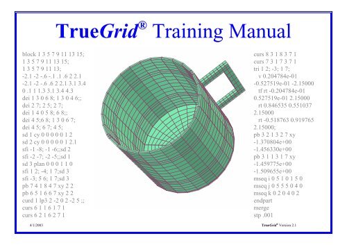
enerate a cup 

Block 1 3 5 7 9 11 13 15; 

1 3 5 7 9 11 13 15; 

1 3 5 7 9 11 13; 

-2.1 -2 -.6 .6 2 2.1 3.1 3.4; 

-2.1 -2 -.6 -.1 .1 .6 2 2.1; 

0 .1 1.1 1.3 3.1 3.4 4.3; 


Block Command with Regions to Delete 



Regions to be Deleted 

The blue regions in these pictures are the 

unneeded regions to be deleted. See if you 

can delete these regions using only 5 deletions. 

Highlight the regions using the index 

bars in the computational window. Then 

click on the Delete button in the Environment 

window. 



Project to the Cylinders 

The inner an outer faces are projected onto the inner and outer cylinders 

with two commands. 



Four ways to Close the Gaps 

Construct a diagonal plane and 

project two opposing faces to 

that surface. 

Change the initial x and y-coordinates 

of two opposing faces so that both faces 

are on the diagonal before the project to 

the cylinders occurs. If they both start 

out the same, they both end up in the 

same place. Use the PB command for 

this. 



Construct a vertical line 3D curve 

at one of the diagonal positions 

using the CURD command. Then 

attach the vertical edges of the 

two opposing faces to this curve 

This also changes the initial 

position of the faces before 

they are projected to the 

cylinders. Treat both opposing 

faces equally. 

Change the initial coordinates 

of a face by rotation. Select the 

face, select rotation in the 

environment window, set the 

angle of perspective to 0, 

restore the picture so that you 

get the view you see here, and 

then rotate. This is done by 

starting the mouse at the center 

and then click and drag to get 

the desired rotation. 


The last step is to use the MSEQ 

command to add more elements 

to round out the model. Take care 

to add matching number of 

elements in the regions that were 

folded together. 


Move the remaining two edges to the 

same position as the opposing edges. 

This is done by selecting pick by node 

in the pick panel and deselecting the 

z-coordinate. Highlight one of the edges, 

pick a node of the opposing edge, and 

attach. Only the initial x and 

y-coordinates are changed. Do this for 

both edges. 


Block Boundaries 

The bb (block boundary) command has many uses. It is perhaps the second 

most important feature. It is used to glue two parts together. This by-passes 

the projection to surfaces. It is used to: 

1. Glue 2 parts together 

2. Form a normal gap between 2 parts 

3. Force periodicity in the mesh 

4. Smooth the mesh within a part across disjoint regions 

5. Keep disjoint regions of a part together 

Each block boundary is identified by a number. A block boundary is created 

in two steps, using the bb command in both steps and in both instances, the 

same id number is used. The first use identifies the master side of the 

interface. The second use identifies the slave side that is then glued to the 

master side. 

Care must be taken to initialize the slave side so that the mapping of the 

slave to the master is obvious. The vertices of the slave side can be adjusted 

after the bb command has been issued. The number of nodes on the master 

and slave side must be multiples of each other. 


Block Boundaries and Transitions 


The trbb (transition block boundary) command is an alternative to 

the bb command used to select a slave side to a block boundary 

interface. This is valid only between parts. 

The ration of elements at the interface must be selected carefully so 

that in one direction, the slave to master ratio is either 2:4, 4:2, 1:3, 

or 3:1. Anything else will cause an error. The 2:4 and 4:2 ratio 

means that both sides must have an even number of elements. This 

ratio must be satisfied for each block on the slave side. 

To achieve a transition in 2 directions requires an intermediate part 

with transitions at both interfaces. 

The transition row of elements are not generated until the part is 

ended. The only way to see them is to go to the merge phase. 

The above limitations will be lifted (no dates). 

This feature is very useful in transitioning from a coarse to a fine 

mesh. Care must be taken to create a good quality mesh. For best 

results, the interface region should be nearly planer and orthogonal. 



Recipe for success 


Steps below can be arranged in almost any order. If the INSPRT command is used, then order is important since the 

commands after insertion of a partition will cause the numbers referencing the partition to change. Steps performed in the 

CONTROL, PART, and MERGE phase are color coded. 

1. Draw a block diagram of the topology with partitions along features 

2. Break problem into parts and draw topology diagrams for each part 

3. Start TrueGrid ® and select an output option (DYNA3D, ANSYS, MARC, AUTODYN,...) 

4. Import IGES geometry and/or create geometry (IGES, IGESFILE, SD, CURD, LD) 

5. Create one part at a time (BLOCK, CYLINDER) 

6. Delete regions that are not needed (DE) 

RECIPE FOR SUCCESS 

7. Move vertices to key positions (PB, PBS, MB, Q, TR) 

8. Select faces to be attached to previously generated parts (BB, TRBB) 



9. Attach edges to curves or surface edges (CURS, CUR, CURE, EDGE, SPLINT) 

10. Select faces and project to desired surfaces (SF, MS, SSF, PATCH) 

11. Add elements (MSEQ) 

12. Select nodal distributions along edges (RES, DRS, AS, DAS, NDS) 

13. Choose special interpolations or smoothings for problem faces (LIN, TF, RELAX, TME) 

14. Choose special interpolations or smoothings for problem interiors (LIN, TF, RELAX, TME) 

15. Assign loads/materials/ boundary conditions (PR, B, FL,...) 

16. Start the next part (go back to step 5) 

17. Assign material properties and select analysis options (CONTROL, *MATS and *OPTS) 

18. Merge parts together and inspect them (MERGE, STP, BPTOL, PTOL, LABELS, CO, MEASURE) 

19. Write the output file (WRITE) 

RECIPE FOR SUCCESS (cont) 


8 Basic Functions 


It is most important to understand the commands in the Mesh menu, which can be 

simplified by grouping the commands by basic functions. 

1. Mesh Density - mseq 

2. Block Deletion - de ,dei 

3. Intialization - pb, pbs, mb, mbi, tr, tri, q 

4. Edge Shaping - cur, curs, cure, curf, edge, splint 

5. Interpolation - lin, lini, ilin, ilini, tf, tfi, relax, relaxi, tme, tmei, hyr,unifm, unifi 

6. Projection - sf, sfi, ms, patch 

7. Nodal Distributions - res, drs, as, das, nds 

8. Equations - dom, x, y, z, t1, t2, t3 

8 Basic Functions in Part Phase 

Commands with the i suffix use index procession, but otherwise are equivalent 

to the same command without the i suffix. 


CAD/CAM 

CAD/CAM systems and Solid Modelers 

IGES - Initial Graphics Exchange Specification (NIST) 

STEP - standard for Exchange of Product model data (NIST, ISO) 

Viewpoint and STL data 

IGES file format 

Hierarchy of IGES geometry entities 

IGES and IGESFILE commands 

Numbering of surfaces and curves and multiple IGES files 

USEIGES and SAVEIGES commands 

IGES levels and associativity groups 

Tolerances 


TrueGrid’s IGES Filter and Its Applications 

Tangent surfaces, trimmed surfaces, and composite surfaces 

How to deal with gaps and overlaps at mesh intersections 


Polygon surfaces 


Two files with data similar to Finite Element meshes: nodal element files. Each element is associated with a surface 

which is named in the first field on the element definition. 

Nodal coordinate file has the following format: 

1, -3.383404, -0.583990 , 2.585073 

2, -3.187954, -0.598938 , 2.572747 

3, -3.186691, -0.594553 , 2.575749 

4, -3.383906, -0.579564 , 2.587889 

5, 4.597703, -0.602771 , 2.579074 

... 

Element connectivity file has the following format: 

hood 7306 7302 7249 7244 

body 7121 7125 7129 7116 

body 7124 7307 7247 7130 

hood 7301 7298 7253 7250 

hood 7297 7294 7257 7254 

... 

Viewpoint Data Format 


IGES format 


IGES Data Format 

Each file contains String, Global, Directory, Parameter, and Terminator data. Pairs of directory records identify a 

geometric entities by the first number. The second number is a pointer into the parameter data. For example, type 128 is a 

NURBS surface. All geometric entities are algebraic. 

Text messages or comments S 1 

1H,,1H;,, 8Hpack.igs, G 1 

5HANSYS,21HREV 5.0 UP 90292,,,,,,,,,,,,13H9210 5. 6 224,,,,,,; G 2 

128 1 0 0 0 0 0 000000001D 1 

128 0 0 12 0 0 0 SURFACE 0D 2 

126 13 0 0 0 0 0 000000001D 3 

126 0 0 6 0 0 0B-SPLINE 0D 4 

... 

128, 1, 1, 1, 1, 0, 0, 1P 1 

1, 0, 0, 1P 2 

0.000000000000E+00, 0.000000000000E+00, 1.00000000000 , 1P 3 

1.00000000000 , 0.000000000000E+00, 0.000000000000E+00, 1P 4 

1.00000000000 , 1.00000000000 , 1.00000000000 , 1P 5 

1.00000000000 , 1.00000000000 , 1.00000000000 , 1P 6 

-2.27778406141 , -1.31507924098 , 3.13843157742 , 1P 7 

12.5598045656 , 7.25140654689 , -6.74905435536 , 1P 8 

7.52332454819 , 4.34359345309 , 22.7490543554 , 1P 9 

22.3609131752 , 12.9100792410 , 12.8615684226 , 1P 10 

0.000000000000E+00, 1.00000000000 , 0.000000000000E+00, 1P 11 

1.00000000000 ; 1P 12 

126, 1, 1, 0, 0, 1, 0, 3P 13 

... 

186, 737, 1, 0, 0, 0, 0; 739P 2642 

S 1G 2D 740P 2642 T 1 


IGES features 

Lines 

Circular arcs 

Conic arcs 

Parametric spline curves 

NURBS curves 

Composite curves 

Planes including bounded 

Ruled surface 

Surface of revolution 

Tabulated cylinder 

Parametric spline surfaces 

NURBS surfaces 

Trimmed surfaces 

Transformations 

Levels 

Associativity 


IGES Features Supported in TrueGrid ® 


Transformations 


Transformation 

Transformations are used to position, scale, and reflect geometric entities such as surfaces and 3D-curves and to duplicate 

a mesh part. Simple operators are listed in order to from complex transformations. The simple operators are: 

x-transformation mx * x 

y-transformation my * y 

z-transformation mz * z 

translation v * x * y * z 

x-rotation rx 2 x 

y-rotation ry 2 y 

z-rotation rz 2 z 

x-scale xsca F x 

y-scale ysca F y 

z-scale zsca F z 

scale scal F 

xy-reflection rxy 

yz-reflection ryz 

zx-reflection rzx 

reference frame tf X 1 X 2 X 3 

frame to frame ftf X 1 X 2 X 3 Y 1 Y 2 Y 3 

transformation mx 15 rz 45 xsca 2 rz 45 


3D Curves 


3D Curves 

Purpose: 3D curves are used primarily to force a mesh edge on a geometry feature defined by a curve. 

Usage: Only mesh edges and vertices can be attached to 3D curves (know as initialization) 

Types of 3D Curves Interactive 3D Curve Creation 

IGES curve LP3 - Piecewise linear curve of interactively selected points 

Edge of a surface SPLINE - Cubic spline between interactively selected points 

Surface contour TWSURF - Curve automatically created at the intersection 

B-spline of two surfaces; 4 - 10 points, interactively selected, 

NURBS spline are needed to initialize this curve 

2D to 3D conversion COEDG - Create curves from surface edges 

Interpolate between two curves 

Surface or curve point selection 

Parameterized function curve 

Project a 3D curve to a surface 

Project a 3D curve to a surface and smooth 

Arc of a circle (3 points) 

Section of a 3D curve 

Copy and transform a 3D curve 

Combine a set of 3D curves and transform 


The surface on the right has a non-concave boundary and 

an interior feature. 

The mesh on the bottom left, which was projected to this 

surface, does not have an interior mesh line which follows 

the interior feature highlighted in yellow. Also, 

the boundaries of the mesh do not include the convex 

portions of the boundaries of the surface. 

By attaching the boundary of the mesh to the edges of the 

surface and by attaching an interior line of the mesh to the 

3D curve that follows the interior feature, one gets a mesh 

that more accurately represents the surface, as shown on 

the bottom right. 



Cubic splines 


Cubic Spline w/Natural Derivatives - 2 nd Derivatives are 0 at the Endpoints 

Every segment of a cubic spline is a 

parametric cubic polynomial. This spline 

passes through each of the control points. 

There are several options based on the 

properties of cubic spline. The subscript i 

below denotes the ith segment: 

X(t) = ait3 2 

+ bi + cit + di Y(t) = e it 3 + f it 2 + g it + h i 

Z(t) = j it 3 + k it 2 + l it + m i 

where the independent variable t is allowed to range over a short interval Suppose there are n segments in the cubic 

spline. This produces 12n unknowns. There are 6n constraints since the endpoints of each section passes through the 

control points. There are 6n-6 additional constraints imposed so that the curves has two derivatives at the interior control 

points. You can choose the derivative at the end points to impose the remaining 6 constraints. 


To create a spline, choose 

SPLINE 

from the 3DCURVES menu. You 

must be in either the Merge or Part 

Phase for this feature. Select points to 

be entered into the table that appears. 

To save the curve, click on the 

SAVE 

button with the left mouse 

button and type a curve number. Then 

select the QUIT button with the left 

mouse. 


Creating a Cubic Spline 



Control the End Derivatives of a Cubic Spline 

Click on the box next to First End in the Point List window and 

enter the three vector components of the derivative for the first 

end point. To specify the derivative at the other end point, fist 

select the box next to Last End in the Point List window then 

enter the vector components of the derivative. 


Before a new control point can be selected, its position 

in the sequence of control points must be selected. 

Insertion is done after the selected control point. 

There are three ways to select the point of insertion. 

Method 1 - Scroll through the control points with 

the keyboard arrow keys. The mouse must be in the 

Point List window. As you scroll, you will see a 

small box in the picture move from one control 

point to anther. 

Method 2 - Click on the row of the desired control 

point with the left mouse button. 


Inserting a Cubic Spline Control Point 

Method 3 - Move the mouse close to the control point in the picture and push the F5 

function key. 

Method 4 - Enter the control point sequence after the Insert button. Either type the 

return key or click on the Insert button. 

Now select a point in the picture to add a new control point. 

In this example, the fourth control point was selected and a new control point was 

inserted after the fourth. Any additional after this new one until a new insertion point 

is selected. 


Before a control point can be deleted, its position in 

the sequence of control points must be selected. 

There are four methods to deleting control points. 

Method 1- Scroll through the control points with the 

keyboard arrow keys. The mouse must be in the 

Point List window. As you scroll, you will see a 

small box in the picture move from one control point 

to another. 

Method 2- Click on the row of desired control point 

with the left mouse button. 


Deleting a Cubic Spline Control Point 

Method 3- Move the mouse close to the control point in the picture and push F5 

function key. 

Method 4- Enter the sequence numbers of the control points into the from and 

to boxes next to the Delete button. 

Click on the button. 

Delete 

In this example, the fourth control point was selected and deleted from the 

Point List. 



Moving a Cubic Spline Control Point 

Before a control point can be deleted, the Point List window must be taken 

out of the insert mode and the control point must be selected. To get out 

of the insert mode, click the left mouse button on the box next to 

Insert Mode so that the check is no longer in the box. There are 

three ways to select the control point to be moved. 

Method 1- Scroll through the control points with the keyboard arrow 

keys. The mouse must be in the Point List window. As you scroll, you 

will see small box in the picture move from one control point to another. 

Method 2- Click on the row of the desired control point with the left mouse button. 

Method 3- Move the mouse close to the control point in the picture and push the 

F5 function key. 

Select the Move Pts. panel. Then select List Pt. Then select one of 

the methods under the label Constrain to. 

With the left mouse, click and drag in the physical picture to move the control 

point to a new location. In this example, the fourth control point was selected and 

moved in the z-direction. Alternatively, use the 

Pick panel options projection or Z-buffer 

. 


3D Curves Exercise 

Create 2 intersecting cylinders. 

sd 1 cy 0 0 0 1 0 0 2 sd 2 cy 0 0 0 .3 1 0 1.5 

Create a spline curve with points from a cylinder. 


3D Curves Exercise 

1. Hide mode graphics with sdint on for interior contour lines on 

2. 3D Curve > SPLINE 

3. PICK > Z-BUFFER 

4. Select points with the left mouse button 

Notice that the entire spline is not on the cylinder. 

angle 0 dsd 1 rest ry -90 

Project this curve onto the cylinder. 

curd 2 projcur 1 1 ; 

Build a polygonal curve from surface points. 

1. racd dasd rest 

2. 3D Curve > lp3 

3. Click the clear button 

4. Select points with the left mouse button 


Form the curve at the intersection of the two cylinders. 

1. racd rest 

2. 3D Curve > twsurf 

3. Click the clear button 

4. Select points forming a crude approximation 

5. Close the loop using Prepend and Accept 

6. Type the two surface numbers into the window 

Interpolate a curve from two other curves 

curd 5 intcur 2 3 .5 ; 

Create a composite curve with arcs. 


curd 6 lp3 0 0 0; ; 

arc3 seqnc rt 1 0 0 rt [1+1/sqrt(2)] [1-1/sqrt(2)] 0 rt 2 1 0 ; 

arc3 seqnc rt 2 1 0 rt [3-1/sqrt(2)] [1+1/sqrt(2)] 0 rt 3 2 0 ; 

lp3 4 2 0; ; 

Create a pipe surface about this curve. 

sd 3 pipe 6 .3 0 .3 1;; 


Select contours from the surface. 

curd 7 contour 3.1.14 3.0.14;; 

curd 8 contour 3.1.41 3.0.41;; 

curd 9 contour 3.1.68 3.0.68;; 

curd 10 contour 3.1.95 3.0.95;; 

Create interpolated curves for the interior. 






These curves can be used to create a butterfly part by attaching the edges to the curves and projecting to the pipe surface. 

NOTE: Not all of the commands are shown here for the sake of brevity. 

block 1 21;1 3 5 7;1 3 5 7;0 4 -.3 -.1 .1 .3 -.3 -.1 .1 .3 

dei ; 1 2 0 3 4; 1 2 0 3 4; 

curs 1 4 2 2 4 2 7 curs 1 3 1 2 3 1 7 

curs 1 2 1 2 2 1 8 curs 1 1 2 2 1 2 8 

curs 1 4 3 2 4 3 10 curs 1 3 4 2 3 4 10 

curs 1 2 4 2 2 4 9 curs 1 1 3 2 1 3 9 

curs 1 3 2 2 3 2 11 

curs 1 2 2 2 2 2 13 

curs 1 2 3 2 2 3 12 

curs 1 3 3 2 3 3 14 

sfi ; -1 -4; -1 -4;sd 3

TrueGrid Training Manual

You also want an ePaper? Increase the reach of your titles

Delete template?

Save as template?