TrueGrid ® User's Manual, Volume 1

TrueGrid ® User’s Manual 

A Guide and a Reference 

by 

Robert Rainsberger 

VOLUME 1: 

Introduction, Graphical User Interface, and Parts 

Version 2.3.0 

XYZ Scientific Applications, Inc. 

April 6, 2006

Copyright © 2006 by XYZ Scientific Applications, Inc. All rights reserved. 

TrueGrid, ® the TrueGrid ® User’s Manual, and related products of XYZ Scientific Applications, Inc. are copyrighted and 

distributed under license agreements. Under copyright laws, they may not be copied in whole or in part without prior written 

approval from XYZ Scientific Applications, Inc. The license agreements further restrict use and redistribution. 

XYZ Scientific Applications, Inc. makes no warranty regarding its products or their use, and reserves the right to change its 

products without notice. This manual is for informational purposes only, and does not represent a commitment by XYZ 

Scientific Applications, Inc. XYZ Scientific Applications, Inc. accepts no responsibility or liability for any errors or 

inaccuracies in this document or any of its products. 

TrueGrid ® is a registered trademark of XYZ Scientific Applications, Inc. 

Silicon Graphics and SGI are registered trademarks of Silicon Graphics, Inc. 

WINDOWS is a registered trademarks of Microsoft Corporation. 

Unix is a registered trademark of The Open Group. 

Abaqus is a registered trademark of Abaqus, Inc. 

Sun Microsystems is a registered trademark of Sun Microsystems, Inc. 

ANSYS, TASCFlow, AUTODyn, and CFX are a registered trademarks or trademarks of ANSYS, Inc. 

NASTRAN and PATRAN are a trademark and a registered trademark, respectively of MacNeal Schwendler Corporation 

FLUENT and FIDAP are registered trademarks of Fluent, Inc. 

CFD-ACE is a trademark of CFD Research Corporation 

Gridgen is a trademark of Pointwise, Inc. 

NASTRAN is a registered trademark of The National Aeronautics Space Administration 

LSDYNA is a trademark of Livermore Software Technology Corporation 

STARCD is a trademark of CD Adapco Group 

LINUX is a registered trademark of Linus Torvalds 

HP is a trademark of Hewlett-Packard Company 

IBM is a registered trademark of the IBM Corporation 

SUN and SOLARIS are a trademark and registered trademarks, respectively, of the Sun Microsystems, Inc. 

SUSE is a trademark of Novell, Inc. 

Intel is a registered trademark of the Intel Corporation 

AMD is a trademark of Advanced Micro Devices, Inc. 

Some other product names appearing in this book may also be trademarks or registered trademarks of their trademark holders. 

Copyright © 1992-2006 by XYZ Scientific Applications, Inc. All Rights Reserved 

ii April 6, 2006 TrueGrid ® Manual

Preface 

New Features 

Since the publishing of this manual for version 2.1 in December of 2001, there have been numerous 

new releases of TrueGrid ® plus this major release. Below is a list highlighting the most significant 

improvements to TrueGrid ® since that publication. 

! Many improvements have been made to support the LS-DYNA, ANSYS, NASTRAN, 

NE/NASTRAN, ABAQUS, FLUENT, and LLNL codes such as DYNA3D, NIKE3D, and 

TOPAZ3D. 

! The symmetry planes are handled correctly when nodes are found at the intersection of two or 

more symmetry planes. 

! The ACCURACY command now applies to the projection to all IGES geometry. 

! The transition block boundary (TRBB) has been extended to 2-way transitions. 

! The slave side of a TRBB region can have partitions anywhere. 

! The OpenGL standard is used to produce fast, high quality, color graphics on all platforms 

! Color (Fill) graphics is available in the Part phase. 

! There is a new command to define functions. 

! The CYLINDER part can be given any frame of reference. 

! There is a new slice feature and display of multiple conditions in the graphics. 

! The physical and computational window can now move in sync. 

! Singular subfigures in IGES are now supported. 

! The READMESH command can read a FEM from IGES. 

! A new dialogue box (WINDOWS only) opens an IGES file using the browse feature in 

WINDOWS. 


TrueGrid ® ManualApril6, 2006 

iii

! Input strings can be 256 characters. 

! Parameters can be 16 characters long. 

! Many features that have limits now have larger limits. 

! There is now a User's Manual for the TG License Manager. 

! There is a new environment variable used to specify the ports used by TG when a firewall is used. 

! The element MEASURE command has been improved. 

! There are new controls in merging nodes using node sets. 

! The projection method has been improved so that complex dependencies in the mesh are always 

calculated properly. 

! The mesh density can be scaled globally with one command. 

! The uniform smoothing (UNIFM) works for solids and faces and a new feature changes to the 

Neumann boundary condition. 

! There are numerous 3D curve and 3D surface additions. 

! Sets have been extended to include polygons for creating and manipulating polygon surfaces. 

! There is a new type of high accuracy algebraic surface defined by a table of points, known as a 

Hermite parametric spline surface. This new surface can be exported to am IGES file. 

! Trimmed IGES surfaces can now be interpolated to produce mid-plane surfaces. 

! Many surfaces can be offset in a normal directions. 

! A block boundary interface can be defined using a set of coordinates. 

! The session file (tsave) from previous runs are protected from being over written. 

! The computational window has been improved. 

! A point can be transformed using the same transformations applied to replicate a part. This can 

be useful when building a sequence of parametric parts. 


iv April 6, 2006 TrueGrid ® Manual

Documentation 

The following TrueGrid ® documents are available: 

TrueGrid ® User’s Manual Volumes 1 and 2- These are the most important documents which contain 

instructions on the use of TrueGrid ® and a reference for the functionality of each command. They 

are available in PDF format and hard copy. 

TrueGrid ® Examples Manual - This manual has numerous examples from the most basic using only 

one or two commands to full models. There are also sections of command input extracted from larger 

models to be instructive on certain topics. Several full models with annotations are included. All 

examples have color graphics. This is available in PDF format and hard copy. 

TrueGrid ® Tutorial - The documentation is intended to aid a beginning TrueGrid ® user in self paced 

training course. It only teaches enough of TrueGrid ® to build simple meshes. Approximately 6 to 

10 hours are needed to work through this course. This is available in PDF format and in hard copy. 

Introductory TrueGrid ® Training Manual - This is a set of view graphs used in the introductory 

training for TrueGrid ® usually held once a month at the main office for XYZ Scientific Applications, 

Inc. This course can be made available at your facility. The view graphs are available in PDF format. 

Advanced TrueGrid ® Training Manual - This is a set of view graphs and examples used in the 

advanced TrueGrid ® training course held occasionally at the main office for XYZ Scientific 

Applications, Inc. This course can be made available at your facility. The view graphs are available 

in PDF format. A CD is available with the examples. 

TrueGrid ® Output Manual - This manual has all of of the commands and options to define the 

material models and analysis options specific to each output format supported by TrueGrid ® . This 

is available in PDF format. 

TrueGrid ® License Manager Manual - This manual describes the operations of the license manager 

used by TrueGrid ® . It is intended for system administrators. It is available in PDF format. 

RELEASENOTES* - Every minor release of TrueGrid ® does not warrant a new version of the 

manuals. Instead, the improvements are listed in these files which accompany the new version of 

TrueGrid ® . This is available in text and PDF format. 

Install_UNIX - These are the installation instructions for TrueGrid ® for UNIX operating systems. 

It is available in text and PDF format. 


TrueGrid ® ManualApril6, 2006 

v

Install_WIN - These are the installation instructions for TrueGrid ® for WINDOWS operating 

systems. It is available in text and PDF format. 

Install_LINUX - These are the installation instructions for TrueGrid ® for REDHAT LINUX 

operating systems. It is available in text and PDF format. 

Install_OSX - These are the installation instructions for TrueGrid ® for APPLE’s PowerPC running 

the MAC TIGER OSX operating systems. It is available in text and PDF format. 

License - The varies licensing agreements for TrueGrid ® are available in text and PDF format. The 

CD is always shipped with a hard copy of the appropriate agreement. This agreement requires that 

you agree to honor XYZ Scientific Applications’ copyright ownership and authorization of 

TrueGrid ® in order to use TrueGrid ® . 

Updates 

If you are licensed to run the latest version of TrueGrid ® , you can get the latest updates and 

documentation on a CD from XYZ Scientific Applications, Inc. or its distributors. These updates are 

also available on the web for down loading. Please contact XYZ Scientific Applications, Inc. At 

(925) 373-0628 for instructions on down loading from the web. 


vi April 6, 2006 TrueGrid ® Manual

Table of Contents 

Table of Contents .............................................................7 

I. Introduction ..............................................................19 

1. What is TrueGrid ® ?...................................................20 

2. History of TrueGrid ® ..................................................21 

3. Availability ..........................................................23 

Getting Information on TrueGrid ® ....................................23 

Getting a Demonstration Copy of TrueGrid ® ............................24 

Purchasing TrueGrid ® .............................................24 

Hardware Platforms ...............................................24 

4. Getting Started .......................................................25 

Installation on UNIX ..............................................26 

Installation on WINDOWS .........................................26 

Installation on LINUX .............................................26 

Installation on OSX ...............................................27 

Learning TrueGrid ® ...............................................28 

Using the Manual.................................................29 

Getting Help .....................................................29 

5. TrueGrid ® Basic Concepts ..............................................30 

Two Kinds of Mesh ...............................................30 

Making Parts and Merging them into a Model ..........................31 

Regions, Indices, and Reduced Indices ................................33 

6. How TrueGrid ® Works ................................................37 

Topology Of The Mesh ............................................37 

Full Indices......................................................37 

Shape Of The Mesh ...............................................37 

Part Initialization .................................................38 

Projection Method ................................................39 

Advantages of the Projection Method .................................39 

Surface Intersection Method ........................................40 

Command Hierarchy ..............................................41 

Multiple Block Structured Parts......................................42 

Quality Meshes ..................................................42 

Algebraic Methods ................................................43 

Interactivity .....................................................43 

Specifying Multiple Blocks .........................................44 

Initial Coordinates ................................................44 

Cylindrical Coordinate Systems......................................45 


TrueGrid ® ManualApril6, 2006 7

Mesh Density Parameterization ......................................45 

Reduced Indices ..................................................45 

Vertices and Regions ..............................................46 

Index Progressions ................................................48 

Graphical Version of Index Progressions ..............................50 

Examples .......................................................51 

7. Conventions .........................................................56 

8. Running TrueGrid ® ...................................................57 

Execution Environment ............................................57 

Two Modes and Two Input Channels .................................57 

Command Line ...................................................58 

Mesh Generation .................................................61 

Termination .....................................................62 

CAD/IGES Geometry .............................................62 

Miscellaneous ...................................................62 

Phases..........................................................63 

Basic Interactive Session ...........................................64 

II. Graphical User Interface ...................................................68 

1. TrueGrid ® on Various Systems ..........................................69 

SGI UNIX Workstation ............................................69 

COMPAQ & DEC Alpha UNIX Workstation...........................69 

SUN UNIX Workstation ...........................................69 

HP UNIX Workstation.............................................70 

IBM UNIX Workstation ...........................................70 

APPLE UNIX Workstation .........................................70 

INTEL or AMD PC Running LINUX .................................70 

INTEL or AMD PC Running WINDOWS .............................71 

2. TrueGrid Windows ...................................................72 

3. The Text/Menu Window ...............................................75 

Menu Window ...................................................75 

Text Window ....................................................77 

4. Graphics Commands ..................................................78 

ad define a numbered annotation ...........................78 

aad add an annotation to the picture in the physical window .......78 

caption change or toggle caption ...............................79 

daad display all annotations in the physical picture ...............79 

dad display a single annotation in the physical picture ............79 

dads display a list of annotations in the physical picture ...........80 

display display with general hidden-line algorithm .................80 


8 April 6, 2006 TrueGrid ® Manual

draw display without hidden line .............................80 

grid turn reference grid on or off .............................81 

pad position an annotation in the physical picture ...............81 

poor poor man’s hidden line removal .........................82 

postscript activate PostScript output ..............................82 

raad remove all annotations from the physical picture ............83 

rad remove an annotation from the physical picture .............84 

rindex label reduced indices ..................................84 

sdint toggle display of surface interior .........................84 

set define various graphic options ...........................85 

slice slice through the picture................................86 

triad turn triad on or off ....................................86 

tvv color and shaded display ...............................87 

zclip remove front portion from physical picture .................87 

5. Picture Controls ......................................................88 

lmove picture left .....................................89 

r move picture right ....................................89 

u move picture up ......................................90 

d move picture down ....................................90 

rx rotate about the x axis .................................91 

ry rotate about the y axis .................................91 

rz rotate about the z axis .................................91 

trans translate to new center of rotation ........................92 

fix freeze center of rotation ................................92 

unfix return center of rotation to picture ........................92 

scale scale all coordinates ...................................92 

xsclscale x-coordinate ....................................93 

ysclscale y-coordinate.....................................93 

zsclscale z-coordinate.....................................93 

zb zoom back ..........................................94 

zf 

zoom forward........................................94 

angle perspective angle .....................................94 

reso change display resolution...............................95 

restore return to original or fixed view ..........................95 

center fit picture to the screen.................................96 

6. Computational Window ...............................................96 

Selecting Regions and Index Progressions with the Index Bars .............97 

Selecting a Region with Click-and-Drag in the Computational Window .....105 

Index Bar Zone..................................................107 

7. The Environment Window .............................................108 

Choosing the Type of Picture .......................................108 



Selecting the Windows to be Redrawn ...............................111 

phys turn the Phys button on .....................................111 

both turn the Both button on .....................................111 

comp turn on the Comp button ....................................111 

Generating a New Picture .........................................112 

Dynamically Moving the Picture ....................................112 

Labels Panel - Labeling Objects ....................................115 

Pick Panel - Pick an Object ........................................124 

Coordinate System of a Picked Point.................................126 

Pick Panel - Picking a Point by Projection ............................126 

Pick Panel - Pick a Point by Z-buffer.................................127 

Pick Panel - Picking a Node........................................127 

Pick Panel - Picking a Vertex ......................................127 

Pick Panel - Picking Partial Coordinates ..............................129 

Pick Panel - Picking an Edge, Face, or Block ..........................130 

Pick Panel - Creating or Modifying Sets Using the Mouse ...............133 

Display List Panel - Determining What Objects are Drawn ...............141 

Move Pts. Panel - Interactively Moving Regions of the Mesh .............148 

Deleting a Region of the Mesh .....................................156 

Attaching the Mesh to Objects......................................157 

Projecting a Mesh Region to a Surface ...............................165 

The Undo Feature ................................................171 

The History Button...............................................171 

The Resume Command ...........................................171 

8. Dialogue Boxes .....................................................172 

Option Lists ....................................................173 

Numbers, Lists of Numbers, and Text Strings ..........................174 

Parser and Fortran Interpreter ......................................175 

Editing and Syntax Checking .......................................176 

Executing and Quitting Dialogue Boxes ..............................177 

Quick Reference to Keyboard Functions ..............................177 

9. Interactive Construction of 3D Curves ...................................179 

III. Part Commands .........................................................196 

1. Geometry and Topology ...............................................197 

de delete a region of the part ..............................199 

dei delete regions of the part ..............................199 

insprt insert a partition into the existing part ....................199 

mseq change the number of elements in the part ................203 

orpt set shell element normal orientation .....................205 



update save the mesh's present state as the initial mesh ............207 

2. Initial Positioning of Vertices ..........................................208 

mb translates vertices ....................................209 

mbi translates vertices ....................................210 

pb assigns coordinates to vertices ..........................210 

pbs assign coordinates to vertices from a labeled point ..........211 

cooref selects feature in the pbs command ......................213 

tr transform a region of the mesh .........................213 

tri transform regions of the mesh ..........................214 

ilin initial interpolation - not a constraint .....................216 

ilini initial interpolation - not a constraint .....................216 

ma translates vertex before interpolations or projections ........217 

pa assigns coordinate values to a vertex ....................218 

q assigns coordinates of one vertex to another ...............218 

3. Initial Positioning of Edges ............................................219 

cur distribute edge nodes along a 3D curve ...................228 

curf distribute and freeze nodes along a 3D curve ..............229 

cure distribute nodes along an entire 3D curve .................230 

curs independently distribute edge nodes along a 3D curve .......230 

edge distribute nodes along an edge of a surface ................231 

4. Interpolation ........................................................234 

esm 2D elliptic smoothing.................................235 

esmp Add source terms for elliptic smoothing ..................238 

hyr Interpolate multiple regions as one region .................238 

lin Linear interpolation ..................................239 

lini Linear interpolation by index progression .................247 

relax Equipotential relaxation...............................247 

relaxi Equipotential relaxation...............................250 

splint Interpolate edges along cubic splines.....................251 

tf 

Transfinite interpolation...............................252 

tfi Transfinite interpolation, by index progression .............258 

tme Thomas-Middlecoff relaxation .........................258 

tmei Thomas-Middlecoff relaxation, by index progression ........263 

neu Orthogonal boundary smoothing ........................263 

neui Orthogonal boundary smoothing, by index progression ......267 

unifm Uniform smoothing ..................................267 

unifmi Uniform smoothing ..................................271 

5. Projection ..........................................................272 

sf project a region onto a surface ..........................273 

sfi project regions onto a surface by index progression .........276 

spp spherical projection ..................................277 



tmplt create template used by spp ............................279 

patch attaches a face to a 4 sided surface patch ..................279 

ms sequence of surface projections .........................280 

6. Nodal Spacing Along Edges ...........................................282 

res relative spacing of nodes of an edge .....................283 

drs relative spacing of nodes of an edge from both ends .........284 

as absolute spacing of first or last element of an edge ..........285 

das absolute spacing of first and last element of an edge .........286 

nds generalized nodal distributed along an edge ...............286 

7. Equations ..........................................................287 

dom specify the region applied to x=, y=, z=, t1=, t2=, and t3= ....288 

x= assign x-coordinates by evaluating a function ..............288 

y= assign y-coordinates by evaluating a function ..............291 

z= assign z-coordinates by evaluating a function ..............291 

t1= assign a temporary mesh variable by evaluating a function ....291 



8. Edit Commands .....................................................292 

history show the history table ................................293 

actcmd activate a mesh command previously deactivated ...........297 

decmd deactivate a mesh command ...........................297 

undo deactivate the last active mesh command .................298 

9. Select Regions For Display ............................................298 

arg add a region to the display .............................300 

argi add a progression to the display .........................300 

darg display all regions ...................................301 

darged display all edges .....................................302 

rg display a region .....................................303 

rgi display a progression .................................303 

rrg remove a region from display ..........................303 

rrgi remove a progression from display ......................304 

strghlhighlight region .....................................304 

strghli highlight index progression ............................304 

clrghl clear highlighted selection .............................305 

10. Labels in the Picture .................................................305 

labels specify type of label to be displayed .....................305 

11. Displacements, Velocities, and Accelerations .............................306 

fd fixed displacement ...................................306 

fdi fixed displacement by index progression ..................307 

fdc cylindrical fixed displacement ..........................308 

fdci cylindrical fixed displacement ..........................308 



fds spherical fixed displacement ...........................309 

fdsi spherical fixed displacement ...........................310 

frb prescribed nodal rotation ..............................311 

frbi prescribed nodal rotation by index progression .............312 

fv prescribed velocities ..................................313 

fvi prescribed velocities ..................................314 

fvc cylindrical prescribed velocities .........................314 

fvci cylindrical prescribed velocities .........................315 

fvs spherical prescribed velocities ..........................315 

fvsi spherical prescribed velocities by index progression .........316 

bv prescribed boundary surface velocities for NEKTON ........316 

bvi prescribed boundary surface velocities for NEKTON ........316 

acc prescribed boundary acceleration ........................317 

acci prescribed boundary acceleration ........................318 

accc cylindrical prescribed boundary acceleration ...............319 

accci cylindrical prescribed boundary acceleration ...............319 

accs spherical prescribed boundary acceleration ................320 

accsi spherical prescribed boundary acceleration ................321 

dis initial displacement in a region .........................322 

disi initial displacement by index progression .................322 

fvv variable prescribed nodal boundary velocities ..............322 

fvvi variable prescribed nodal boundary velocities ..............324 

fvvc cylindrical variable nodal prescribed boundary velocities .....325 

fvvci cylindrical variable prescribed nodal boundary velocities .....325 

fvvs spherical variable prescribed nodal boundary velocities ......326 

fvvsi spherical variable prescribed nodal boundary velocities ......327 

vacc variable prescribed nodal boundary accelerations ...........327 

vacci variable prescribed nodal boundary accelerations ...........327 

vaccc cylindrical variable nodal prescribed boundary accelerations . . 328 

vaccci cylindrical variable prescribed nodal boundary accelerations . . 328 

vaccs spherical variable prescribed nodal boundary accelerations ...329 

vaccsi prescribed nodal boundary accelerations (spherical) .........330 

rotation part initial rigid body rotation ..........................330 

velocity part initial velocity ...................................330 

ve initial velocity in a region .............................331 

vei initial velocity by index progression .....................331 

12. Force, Pressure, and Loads ............................................332 

arri modify pressure amplitudes and shock arrival time ..........332 

dist laser distribution function .............................336 

csf cross section forces for DYNA3D .......................338 

fa fixed nodal rotations .................................338 



fai fixed nodal rotations .................................338 

fc concentrated nodal loads ..............................338 

fci concentrated nodal loads ..............................339 

fcc cylindrical concentrated nodal loads .....................340 

fcci cylindrical concentrated nodal loads .....................340 

fcs spherical concentrated nodal loads ......................341 

fcsi spherical concentrated nodal loads ......................342 

ll linearly interpolate loads by arc length ...................343 

mdep momentum deposition ................................343 

mom nodal moment about an axis ...........................344 

momi nodal moment about an axis ...........................346 

ndl nodal distributed load .................................346 

ndli nodal distributed load .................................346 

pr pressure load .......................................348 

pri pressure load by index progression ......................348 

pramp pressure amplitudes from a FORTRAN like expression ......349 

13. Boundary and Constraint Commands ...................................351 

b global nodal displacement and rotation constraints ..........351 

bi global nodal constraints, by progression ..................353 

cfc convective flow (CF3D) output boundary conditions ........354 

cfci CF3D output boundary conditions by progression ..........354 

fbc FLUENT boundary conditions ..........................356 

fbci FLUENT boundary conditions by index progression ........356 

jt assign a node to a numbered joint .......................357 

il identifies an inlet for fluid flow. ........................359 

ili identifies an inlet for fluid flow, by index progression .......360 

lb local nodal displacement and rotation constraints ...........360 

lbi local nodal boundary constraints, by progression ...........360 

mpc shared nodal (multiple point) constraints for a nodal set ......361 

namreg name a region for the TASCFLOW output file .............362 

namregi name regions for the TASCFLOW output file ..............363 

nr non-reflecting boundary ...............................363 

nri non-reflecting boundaries .............................363 

ol identifies a face of the mesh as an outlet for fluid flow .......363 

oli identifies faces of the mesh as an outlet for fluid flow .......364 

reg select a region for the REFLEQS boundary condition ........364 

regi select regions for the REFLEQS boundary condition ........364 

sfb locally constrain face nodes ............................365 

sfbi locally constrain face nodes by progression ................366 

sw assign nodes that may impact a stone wall .................366 

swi assign nodes that may impact a stone wall .................367 



syf assign faces to a numbered symmetry plane with failure ......367 

syfi assign faces to a numbered symmetry plane with failure ......367 

trp create tracer particles for Lsdyna ........................368 

14. Radiation and Temperature Commands ..................................368 

bf bulk fluid ..........................................368 

bfi bulk fluid by index progression .........................369 

cv boundary convection .................................369 

cvi boundary convection .................................369 

vcv boundary convection with functional amplitudes ...........370 

vcvi boundary convection with functional amplitudes ...........370 

cvt convection thermal loads ..............................371 

cvti convection thermal loads ..............................371 

flprescribed boundary flux ..............................371 

fli prescribed boundary flux ..............................372 

vfl prescribed boundary flux with functional amplitude .........372 

vfli prescribed boundary flux with functional amplitude .........372 

ft 

prescribed temperature................................373 

fti prescribed temperature by progression ...................373 

vft functional prescribed temperature .......................373 

vfti functional prescribed temperature by progression ...........374 

hfl specify flows and fluxes ...............................374 

hfli specify flows and fluxes, by index progression .............375 

inizone initial conditions for the REFLEQS option ................375 

inizonei initial conditions for the REFLEQS option, by progression ...376 

setsor set REFLEQS source terms ............................376 

setsori set REFLEQS source terms, by index progression ..........377 

rb prescribed radiation boundary condition ..................378 

rbi prescribed radiation boundary condition, by progression .....378 

vrb prescribed radiation boundary w/ functional amplitudes ......378 

vrbi prescribed radiation boundary, by progression .............379 

re radiation enclosure ...................................379 

rei radiation enclosure by index progression ..................380 

te constant nodal temperature ............................380 

tei constant nodal temperature ............................381 

temp part default constant nodal temperature ..................381 

tepro variable nodal temperature profile .......................381 

tm initial temperature condition ...........................382 

tmi initial temperature condition by index progression ..........382 

vtm initial temperature w/ functional temp ....................382 

vtmi initial temperature by index progression w/ functional temp ...382 

vhg volumetric heat generation.............................383 



vhgi volumetric heat generation by index progression ...........383 

vvhg volumetric heat generation w/ functional amplitude .........383 

15. Electric Condition Commands .........................................383 

efl electric flux boundary condition ........................383 

efli electric flux boundary condition by index progression .......384 

mp constant magnetic potential ............................384 

mpi constant magnetic potential ............................384 

v electrostatic potential boundary condition .................384 

vi electrostatic potential boundary condition .................384 

16. Springs, Dampers, and Point Masses ....................................385 

npm creates a node with a point mass ........................385 

pm point mass to a vertex of the present part .................386 

spdp assigns a face to be half of a set of spring/damper pairs ............386 

spring create/modify a spring ................................387 

17. Interfaces and Sliding Surfaces ........................................389 

bb block boundary interface ..............................389 

trbb slave transition block boundary interface .................395 

inttr trbb interpolation parameter ............................404 

dbb display a block boundary in the picture ...................404 

rbb remove a block boundary from the picture ................404 

abb add a block boundary to the picture ......................405 

dbbs display a set of block boundaries in the picture .............405 

rbbs remove a set of block boundaries from the picture ..........405 

abbs add a set of block boundaries to the picture ................405 

dabb display all block boundaries ............................405 

rabb remove all block boundaries from the picture ..............405 

bbint block boundary interior mesh lines ......................406 

flowint create named regions for the CFX output file ..............406 

flowinti create named regions for the CFX output file ..............407 

iss save interface segments ...............................407 

issi save interface segments ...............................407 

si assign sliding interface to region ........................408 

sii assign sliding interfaces ...............................409 

shtoso shell to solid interface ................................411 

shtosoi shell to solid interface by progressions ...................412 

18. Element Cross Sections ..............................................413 

n set orientation of normals on shells ......................413 

or orientation of element local coordinate axes ...............414 

ssf project shell onto an interpolated surface .................414 

ssfi project shell onto an interpolated surface, by progression .....415 

th thickness of shell ....................................415 



thi thickness of shell ....................................416 

thic default shell thickness ................................416 

19. Beams ............................................................417 

ibm generate beams in the i-direction ........................417 

ibmi generate beams in the i-direction by index progression .......420 

jbm generate beams in the j-direction ........................424 

jbmi generate beams in the j-direction by index progression .......425 

kbm generate beams in the k-direction .......................429 

kbmi generate beams in the k-direction by index progression ......432 

20. Diagnostics Commands ..............................................437 

mea choose a way to measure mesh quality ...................437 

meai choose a way to measure mesh quality ...................438 

21. Parts Commands ...................................................439 

cycorsy frame of reference for cylinder part ......................439 

endpart complete the part and add it to the data base ...............440 

savepart save all part data in a parts data base .....................441 

22. Replication of Parts .................................................441 

lrep local replication of a part ..............................442 

grep global replication of a part .............................445 

23. Merging of Parts ....................................................446 

fn tied node sets with failure .............................449 

fni tied node sets with failure .............................451 

24. Output Commands ..................................................451 

epb element print block ..................................451 

npb nodal print block ....................................451 

supblk select regions to be combined in the block structured output ........451 

25. Sets ..............................................................453 

delset delete a set .........................................453 

eset add/remove elements to/from a set of elements.............454 

eseti add/remove elements to/from a set of elements.............455 

fset add/remove faces to/from a set of faces ...................455 

fseti add/remove faces to/from a set of faces ...................457 

nset add/remove nodes to/from a set of nodes ..................458 

nseti add/remove nodes to/from a set of nodes ..................458 

nsetc attach a comment to a node se ..........................460 

fsetc face set comment ....................................460 

esetc element set comment .................................460 

nsetinfo report the node set names and number of nodes ............460 

26. Material Commands .................................................461 

mate part default material number for each region ..............461 

mt material number for a region ...........................461 



mti assign material number ...............................462 

mtv material number assigned to a specified volume ............466 

por to specify the region with porosity for REFLEQS ...........469 

pori to specify the region with porosity for REFLEQS ...........470 

sc to define the ale smoothing constraints for LS-DYNA3D .....470 

IV. Index ..................................................................471 



I. Introduction 



1. What is TrueGrid ® ? 

TrueGrid ® is a powerful, interactive and batch, mesh generator. It can create meshes of unsurpassed 

quality more quickly and easily than by any other method.With this tool, you can generate meshes 

for finite difference and finite element simulation codes that model the behavior of fluids and 

structures. However, it is more than a mesh generator – it can generate complete input files for many 

simulation codes. 

TrueGrid ® is fundamentally a parametric mesh generator. This means that you can make a change 

to a parameter and rerun the commands that form a mesh to get a new mesh reflecting the change. 

This is a non-trivial feature that affects the way you build the mesh. The Graphical User Interface 

has been designed so that you can issue commands without parametric considerations. Underlying 

this simplified use of the commands is a parametric engine waiting for you to discover, once you 

have become familiar with the basic capabilities. The session file (the default name is tsave) is 

automatically generated each time you run TrueGrid ® to record every command needed to reproduce 

your mesh. This is why you always have the option to run a command file when you start TrueGrid ® . 

This is also why there is a keyword command for everything you do in TrueGrid ® . This is perhaps 

a subtle distinction, but when a new feature is added to TrueGrid ® , it is formed as a parametric 

keyword driven command. Then the Graphical User Interface is added to make it easier to use. The 

Graphical User Interface is just a shell around TrueGrid ® and can be bypassed by using the nogui 

option on the execute line. 

TrueGrid ® generates multi-block structured meshes (see the block and cylinder commands). Each 

block is composed of solid hexahedral (six-sided) elements and/or structural quadrilateral shell and 

beam elements (see the bm, ibm, jbm, and kbm commands) arranged in rows, columns, and layers. 

In degenerate cases, the solid elements are wedges or tetrahedrons as the case may be. Shells can 

degenerate to triangles where the geometry requires. Typically, one creates a mesh using the block 

or cylinder part several times and with the requirement that these parts are connected. This is easily 

done using the block boundary interface commands bb and trbb which will glue one block or 

cylinder to another. These commands can also be used to form one mesh from two independently 

generated meshes. 

TrueGrid ® can generate meshes that match your geometry using various surfaces and curves, such 

as those defined by you from an extensive built-in library (see the sd and curd commands). These 

surfaces and curves can be derived from experimental (see the vpsd command and the lp3 option 

of the curd command) or computational data (see the mesh, face, and faceset options of the sd 

command), from CAD/CAM programs via IGES files (see the iges command), or form drawings 

using algebraic forms (most options of the sd, curd, and ld commands). You can also combine 

surfaces (see the sds option of the sd command) and curves (see the coedge or the sdedge option of 

the curd command). The projection method will place the block structured mesh to intersections or 



other combinations of surfaces and curves (see the sf, pb, mb, and curs commands). 

Some of the tools for generating high quality meshes include multi-linear interpolation (see the lin 

command), transfinite interpolation (see the tf command), and elliptic smoothing (see the relax, 

unifrm, tme, and esm commands). Diagnostic tools make it easy for you to measure the quality of 

your mesh (see the mea command). Then you can make local or global changes to the mesh to 

improve the quality, if desired. 

TrueGrid ® features a graphical user interface that lets you generate your mesh by `pointing and 

clicking`. Prompts, dialogue boxes, and an on-line help package help you create your mesh. You 

learn how to use the tool by using it. You can view the mesh as you build it. The arbitrary undo and 

redo facility lets you easily experiment with modifications to the mesh. These interactive features 

are designed to give you the fast feedback you need to speed up the mesh generation process. 

To know the commands mentioned above is to know the core commands in TrueGrid ® to generate 

a mesh. You can easily learn to use the other commands in TrueGrid ® as the need arises. 

TrueGrid ® is currently available on many 

Unix workstations such as SUN, IBM 

RS/6000 series, HP 9000/700 series, 

COMPAQ/DEC, and SGI workstations. It 

is also available on Personal Computers 

running all variations of Windows and 

LINUX. This includes SUSE LINUX on the 

AMD Opteron and OSX on the APPLE. 

2. History of TrueGrid ® 

TrueGrid ® evolved from a line of mesh 

generators that started with the INGEN 

mesh generator. INGEN was developed at 

Los Alamos National Laboratory in the late 

1970's by William Cook to generate meshes 

for finite element simulation codes. 

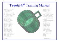
INGEN is composed of surface and two Figure 1 Mesh of Cockpit 

dimensional region generators that use 

linear-blending formulae developed by Coons. INGEN uses the i, j indexing scheme to number 

nodal points and to construct elements. An important INGEN innovation is indirect indexing which 

provides a parameterized mesh capability. This allows the mesh to be refined without altering all 



of the input. 

The INGRID mesh generator came next in the line. INGRID development began at the University 

of Tennessee in 1979 and was initially based on INGEN. Usage of INGEN had shown simple 

patterns of commands that were frequently used. 

The next phase of INGRID development began at Lawrence Livermore National Laboratory. Doug 

Stillman , John Hallquist, and Robert Rainsberger were contributors to INGRID. The availability 

of supercomputers and the increased efficiency and capabilities of the simulation codes drove this 

development. The concept of index progressions was added to provide a concise and simple method 

for describing complex structures. A limited projection method was added. MAZE 2D curve 

generation capabilities were implemented as well as MAZE parts which simplified the modeling of 

many geometries. Commands were added that made it easy for the user to generate descriptions of 

boundary conditions, loads, and material properties for several simulation codes on an individual 

basis. 

Figure 2 

Mesh of Fixture Key 

INGRID was used as the starting point for 

the development of TrueGrid ® . While 

TrueGrid ® incorporates al most al l of 

INGRID's features, TrueGrid ® 's 

improvements and new features go far 

beyond INGRID's scope. Only a small 

fraction (about 2.5%) of TrueGrid ® 

actually comes from the 1990 version of 

INGRID. 

TrueGrid ® 's graphical user interface and 

mesh visualization tools let you see results 

at every step of the generation process. A 

command history feature was incorporated 

to let the user inspect commands as well as 

turn them on or off in order to see their 

effects and debug the mesh. Thus 

TrueGrid ® seamlessly mixes its interactive 

mode with a batch mode. This interface is 

designed to make it easy for you to see not 

only the physical mesh of x,y,z coordinates, but also the simulation code's discrete computational 

mesh of i,j,k coordinates. With TrueGrid ® , you can define and transform the physical mesh by 

referring to either the physical or the computational mesh. Both meshes are displayed, and the 

TrueGrid ® highlighting tool allows the user to select regions in the computational mesh and see the 



corresponding regions in the physical mesh highlighted. 

The easier it is to make modifications to the 

mesh, the faster you can complete it. One way 

that TrueGrid ® makes modifications easy is 

with extensive parameterization capabilities. 

Surfaces, curves, mesh density, and mesh 

topology can be defined by using parameters, 

Fortran like algebraic expressions, functions, 

and conditional statements. Surfaces and 

curves can be referenced symbolically. 

Modifying the mesh then becomes a matter of 

modifying relatively few parameters.For more 

complex and accurate meshes, the XYZ team 

programmed TrueGrid ® to provide access to an 

extensive set of predefined surfaces plus 

CAD/CAM NURBS surfaces imported via 

IGES-formatted files. In addition, there are 

Figure 3 Mesh of L-Bracket 

several ways for the user to define their own 

surfaces. TrueGrid ® 's flexible geometry 

concept lets the user combine these surfaces in 

any way. The surfaces do not have to meet smoothly; they can overlap or not meet at all. Using a 

sophisticated projection method, TrueGrid ® will match the mesh to the surfaces. 

3. Availability 

Getting Information on TrueGrid ® 

You can get information or help on TrueGrid ® 's capabilities, including descriptions of its meshing 

and geometry methods, graphical user interface, and connections to simulation codes by calling: 

or by faxing to: 

or by writing to: 

(925) 373-0628 

(925) 373-6326 



XYZ Scientific Applications, Inc. 

1324 Concannon Blvd. 

Livermore, CA 94550 

or by e-mailing to: 

or by visiting our web site at: 

info@truegrid.com 

http://www.truegrid.com 

Getting a Demonstration Copy of TrueGrid ® 

Currently, we offer a TrueGrid ® demonstration program that will run on a Windows PC. This 

program is available on our home page and shows you several example meshes which are generated 

using TrueGrid ® . 

In addition, a trial version of our software may be obtained by contacting our office using one of the 

above means. This time-limited trial includes our Tutorial, User’s, Examples, Output, and License 

Manager manuals which will help you explore TrueGrid ® ’s powerful mesh-generation method and 

its sophisticated graphical user interface as you generate sample meshes of your own. 

Purchasing TrueGrid ® 

TrueGrid ® licenses can be purchased on a yearly basis or perpetual (paid-up). Both include any 

upgrades during the year of purchase. There is an additional cost to maintain TrueGrid ® beyond the 

first year for a perpetual license. Call, write or e-mail XYZ Scientific Applications to get pricing or 

further licensing information on TrueGrid ® . 

Hardware Platforms 

TrueGrid ® is currently available on the following computers: 

* Silicon Graphics, Inc. workstations running UNIX 

* SUN and SUN-compatible workstations running UNIX 

* IBM workstations running UNIX 

* COMPAQ/DEC workstation running UNIX 

* HP workstation running UNIX 



* Intel PC compatible running WINDOWS or REDHAT/SUSE LINUX 

* AMD Opteron running SUSE 

* APPLE POWER PC running OSX 

Call or write XYZ for details on hardware 

and software requirements. 

4. Getting Started 

The installation instructions describes stepby-step 

how to install and configure 

TrueGrid ® for your particular platform and 

environment. These instructions are 

included in all distribution CDs. Key points 

for each installation are included here for 

completeness. Full details can be found in: 

Install_UNIX.txt or Install_UNIX.pdf for 

the UNIX operating systems 

Install_WIN.txt or Install_WIN.pdf for the 

WINDOWS operating systems 

Install_LINUX.txt or Install_LINUX.pdf 

for the REDHAT LINUX operating systems 

Figure 4 

Mesh of Surface of Dodecahedron 

Install_OSX.txt or Install_OSX.pdf for the OSX operating systems 

If your machine is not authorized to run this version TrueGrid ® , then the installation or registration 

program will request an authorization code from XYZ Scientific Applications. You will be asked 

to send a company name, a check sum, and a machine ID number presented to you by the installation 

or registration program. In response, XYZ Scientific Applications will return an appropriate 

authorization code with a new check sum. When this is entered, the machine will be authorized and 

the TrueGrid ® License Manager will be (re)started. It may be necessary to set the TGHOME 

environment variable so that TrueGrid ® executable program, called tg, will know where the 

authorization file, .tgauth, and the data files are located. 

This license manager must be on one machine in a network. Then TrueGrid ® can be run from any 

machine on the network. When installing TrueGrid ® on a machine that is not running the license 

manager, simply copy the .tgauth file from the licensed machine into the TrueGrid ® installation 



directory on this new machine. 

Installation on UNIX 

You will probably need to be root to make this installation. Change directories to the directory for 

TrueGrid ® . Execute the setup program on the CD-ROM that is designed for the machine on which 

you are running by specifying the full name of the executable. For example, if the CD-ROM is 

mounted on /cdrom and you are installing on an SGI workstation, then execute 

/cdrom/tg23_sgi.exe 

If you have been instructed to download an executable from our web page, then you should know 

that it is the same file as just described. After downloading the file, you will need to add execute 

permissions. Then, you should execute it in the installation directory. 

Installation on WINDOWS 

If you download from the Internet, then you must double click on the file name/icon for the 

self-extracting archive file to un-compress. Then change directories (click on the new folder). On 

a distribution CD, change directories or folder to WINDOWS. 

Run SETUP.EXE in order to install TrueGrid ® . You can install TrueGrid ® in any directory or folder 

which does not have a space in its name or its path. The default is C:\TrueGrid. If you choose a 

directory other than the default, you will need to set the environment variable TGHOME so that 

when TrueGrid ® is run, it will know where the .tgauth, menu, and dialogue files are located. 

Installation on LINUX 

This installation uses the "unzip" utility to extract the TrueGrid ® files from the given archive file. 

The files extracted will reside in the TrueGrid ® directory (typically /usr/TrueGrid). 

No effort is made to create this directory or set permissions on it. Rather, the user is responsible for 

this. The environment variable TGHOME must be set to this directory.(e.g., in csh and tcsh use 

"setenv TGHOME /usr/TrueGrid", in sh and bash use "set TGHOME=/usr/TrueGrid; export 

TGHOME=/usr/TrueGrid" .) The setting of the environment variable, TGHOME should be put in 

the .cshrc (for csh and tcsh) and .bashrc (for sh and bash) of each TrueGrid ® user. 

The Sentinel Rainbow Drivers are required for the license manager to run properly. Without them 

the license manager will lock up the system requiring a manual powering down. To check to see if 

the drivers are installed, type "ls /dev/rnbodrv*". If nothing is listed, the drivers need to be installed 



and root privileges will be required. (Note: USB dongles are not supported for RedHat Linux 7.2 to 

8.0 and parallel port driver are not available for RedHat Linux Enterprise 4.0 or SUSe.) 

These drivers are provided by Rainbow in "rpm" format so the RPM Package Manager is also 

needed. (This is already available in most Linux (all RedHat Linux) installations.) 

Different Rainbow drivers are needed depending on the version of RedHat (or comparable) Linux. 

If you are not using RedHat or Suse, you need to pick the kernel level which best matches the kernel 

levels below: 

RedHat 7.2 to RedHat 8.0(Kernel version 2.4.7 to 2.4.18): tg23_RH8.ZIP 

RedHat 9.0: 

(Kernel version 2.4.20 ): tg23_RH9.ZIP 

32 bit RedHat Enterprise 4.0 and SUSe 9.3 (Kernel version 2.6.5 to 2.6.11): tg23_EN4.ZIP 

64 bit SUSe 9.3 (Kernel version 2.6.11): tg23_SU9.ZIP 

Once the TrueGrid ® software is unpacked and the Rainbow drivers are installed, run tgauth in the 

TrueGrid ® directory to turn on the authorization. 

Installation on OSX 

This procedure uses the "unzip" utility to extract the TrueGrid ® files from the given archive file. The 

files extracted will reside in the TrueGrid ® directory (typically /usr/TrueGrid). No effort is made to 

create this directory or set permissions on it. Rather, the user is responsible for this. To create 

/usr/TrueGrid, open a terminal or X window and change directory to /usr (cd /usr). Then create the 

TrueGrid directory ("sudo mkdir TrueGrid"). Make sure you have the owner and 

group ids set to what you want ("sudo chown : TrueGrid") and the 

permissions set ("sudo chmod -R a+r TrueGrid"). 

The environment variable TGHOME must be set to this directory.(e.g., in csh and tcsh use "setenv 

TGHOME /usr/TrueGrid", in sh and bash use "set TGHOME=/usr/TrueGrid; export 

TGHOME=/usr/TrueGrid" .) The setting of the environment variable, TGHOME should be put in 

the .cshrc (for csh and tcsh) and .bashrc (for sh and bash) of each Truegrid user. 

The Sentinel Rainbow Drivers required for the license manager to run properly. To see if the Drivers 

are installed, check to the existence of the /Library/Extensions/Sentinel.kext/ (with a non-empty 

Content subdirectory). 

If the drivers are not installed, you can do so with the Mac OSX installer in /usr/sbin. Go to the 

RAINBOW subdirectory (i.e. cd RAINBOW) of your TrueGrid ® directory and type (all on one line) 



sudo /usr/sbin/installer -pkg SentinelDriver1.0.0.pkg/ -target /Library/Extensions/Sentinel.kext 

Please note that you need administrative privileges to do this installation and will need to restart your 

machine before the drivers become available. 

Once the TrueGrid ® software is unpacked and the Rainbow drivers are installed, run tgauth in the 

TrueGrid ® directory to turn on the authorization. 

There are two features of OSX which need to be addressed. 

First, you should run TrueGrid ® from an X11 window application (X11.app) rather than the 

Terminal application (Terminal.app). Second, most TrueGrid ® user perfer the window focus to 

follow the mouse rather than having to bring the window to the front to get focus. To get your X 

windows to use the focus follows the mouse, you need to type: 

defaults write com.apple.x11 wm_ffm true 

in and Xterm or terminal to reset focus. You will need to log out of the X11 session before it can 

take effect. 

Learning TrueGrid ® 

Be sure to read the sections ``TrueGrid ® Basic Concepts``and ``How TrueGrid ® Works``. These 

sections introduce you to the concepts and notations of TrueGrid ® . 

Also work through the TrueGrid ® Tutorial manual. This takes you step-by-step through the 

generation of a model. After this tutorial, you will have the fundamental skills needed to use 

TrueGrid ® . 

Next, read the section ``Running TrueGrid ®``. After reading this section, you will have an 

understanding of the general sequence of actions you and TrueGrid ® will perform to generate your 

mesh. Expand this reading to include the rest of the Introduction and the chapter on the Graphical 

User Interface (GUI). Some advanced users prefer to type the commands in the text window or 

create a batch file, but the GUI can be a tremendous aid for the new user. 

Finally, look at the documented examples which are provided in the Examples directory along with 

the distribution. You can use any text editor to view these annotated files while you examine them 

on the screen. Insert interrupt commands in order to pause execution at key locations and then click 

the Resume button in order to continue execution. At this point, you should be able to set up simple 



models with TrueGrid ® , and modify more 

complicated models set up by other people. 

Using the Manual 

The manual is organized into seven (7) 

chapters. This chapter, the Introduction, 

has basic information on TrueGrid ® as well 

as more advanced information that applies 

to TrueGrid ® as a whole. The second 

chapter describes the Graphical User 

Interface, which is as important to 

understand as the Introduction chapter. 

The next four chapters serve as a command 

reference with complete descriptions of all 

of TrueGrid ® 's commands and features. 

The Part Commands chapter covers the 

commands that are used to initially generate 

Figure 5 Mesh of a Chain 

the mesh and impose constraints, loads, and 

conditions. The Geometry Commands chapter discusses how you can use TrueGrid ® to generate and 

manipulate the geometry of your part(s) prior to attachment or projection. The Assembly Commands 

chapter describes the means of combining different parts into a complete model, verifying it, and 

creating a formatted output file. The Global Commands chapter describes commands which can be 

used in all phases of a model’s development. Notice that these first 3 chapters roughly correspond 

to the three phases in TrueGrid ® and then the Global chapter contains commands common to all 

three phases. The Output chapter contains the keyword commands used to control the output format. 

Detailed information about the material models and analysis options can be found in the TrueGrid ® 

Output Manual. 

If you know the name of a command and want information on it, the index is the quickest way to find 

it. If you are looking for a particular capability, you can either look for an appropriate keyword in 

the index or else try the table of contents. The manual's table of contents is an excellent place to look 

for a capability since it includes, with every command name, a brief description of what the 

command is used for. 

Getting Help 

For help, call (925) 373-0628 or email at info@truegrid.com. If possible, please include an input 

file which exhibits the difficulty that you are having. 



5. TrueGrid ® Basic Concepts 

This section will discuss some of the concepts and notations which permeate TrueGrid ® . 

Two Kinds of Mesh 

Figure 6 Physical mesh of the Block with 

spline interpolated edges 

Figure 7 Computational mesh of the Block 

with 8 SubBlocks 

In TrueGrid ® there are two representations of a mesh: physical and computational (Figure 6 and 

Figure 7). The physical mesh lies in the physical space where you want to model something, while 

the computational mesh lies in an abstract space with only integer valued points. There is a 

correspondence between every node in the computational mesh and the corners of the blocks, usually 

referred to as vertices or control points, of the mesh You move the physical mesh to fit the real 

object you are modeling. In contrast, the computational mesh does not move. The computational 

mesh serves as a convenient way of identifying regions of the mesh which are to be the object of 

varies functions. Object in the physical space have three coordinates named x, y, and z. Objects in 

the computational space have three coordinates or indices named i, j, and k. From a mathematical 

perspective, a mesh is a vector function that maps a three dimensional region (the computational 

mesh) to a three dimensional region (the physical mesh). Every point in the mesh has six coordinates, 

three indices and three physical coordinates. We will only be interested in indices with integer 

values, although one can extend the notion of a computational mesh to all reals for a theoretical 

discussion. 



Making Parts and Merging them into a Model 

A typically mesh will be complicated enough that it is easier to build by first making a number of 

parts and then putting these parts together. Each part begins as a rectangular set of nodes called a 

block (see the commands block, cylinder, and blude). You can then move (see the commands pb, 

mb, mbi, tr, and tri) and deform (see the commands sf, sfi, cur, curs, cure, curf, and edge) this 

simple block structure into the shape of the part you need (Figure 10, Figure 11, Figure 12 and 

Figure 13). There are function that control the interpolation (see the commands res, drs, as, das, 

lin, lini, tf, tfi, relax, relaxi, tme, tmei, unifm, and unifmi) of interior nodes. Some functions affect 

the mesh in both physical and computational space, e.g. deleting regions of the mesh (see the 

commands de and dei) or making copies (see the commands lrep, grep, pslv, and pplv). Once you 

have made all the parts, you can join them by merging (see the commands merge, t, tp, and stp) 

coincident nodes (Figure 9 and Figure 8). 

Figure 8 

Completed model of fictional spaceship 

In TrueGrid ® , the most important way to deform a simple mesh is with the sf or sfi commands. This 

is done, interactively, with the PROJECT button. For a projection, you specify a region of the mesh 

and a surface to project it onto. For every node of the region in physical space, TrueGrid ® will find 

its projection onto the surface, i.e. the closest point on the surface. That projection point will be the 

new location of the node in physical space. (See the discussion of the sf command for a more precise 

description.) But TrueGrid ® is not finished when it has moved the face of a block part. Every other 

node of the part may have to be moved in order to preserve interpolation and spacing rules. 



Figure 9 

Model of a fictional spaceship, before merging parts 



Figure 10 Simple Part before Projections 

Figure 11 

Cylindrical Surfaces 

For example, we specified that the upper face of the block in Figure 10 be projected to the upper 

cylinder in Figure 11 in order to get the curved upper face of Figure 13. After this surface projection, 

TrueGrid ® automatically moved all of the neighboring interior nodes upwards in order to 

satisfy the interpolation rules. 

To repeat, projections are a way to define the shape of a part by placing its face nodes onto surfaces. 

The interior nodes are placed by interpolation. By default, TrueGrid ® places interior nodes with a 

linear interpolation method. This is discussed in detail in the remarks on the lin command. You can 

specify other interpolation algorithms if you prefer. (Figure 13 was made with the tf transfinite 

interpolation command.) 

Regions, Indices, and Reduced Indices 

When you define a mesh with TrueGrid ® , you often refer to a region, i.e. a set of nodes which form 

a rectangular set in the computational space. A region may be a vertex, edge, face or volume of the 

mesh. 

One of the major notational issues is how to specify a region. We do not want to specify a region 

directly, by giving the lower and upper limits for its i, j, and k indices. This is because we may later 

want to change the number of nodes in the mesh. If we specified regions in terms of the actual i, j, 

and k index values, we couldn't change the number of nodes (see the command mseq) without 

carefully going through the entire mesh specification and changing index values in each of the many 



places that refer to some region. 

TrueGrid ® solves this problem by describing the computational space with two sets of indices at 

once: full indices and reduced indices. 

The indices are the coordinates in computational space and change if you refine the mesh without 

otherwise changing the shape. The block, cylinder, and blude commands create a three dimension, 

multi-block structured, rectangular mesh. The numbering of the nodes in each direction is 

independent, starting with 1. This produces a three dimensional array of nodes. Each node in 

uniquely identified by the three indices i, j, and k. For example, 

block 1 5;1 6;1 7; ... 

creates a simple block mesh of 5 by 6 by 7 nodes in the i, j, and k directions respectively. The 

semicolon terminates the i, j, and k index lists. The block, cylinder, and blude commands are 

generalized so that a single part can have any number of connected blocks. These parts usually 

contains more blocks than are needed for a particular problem. This is because it is usually easier to 

define an array of blocks and delete some of them then it is to define each required block separately. 

For example: 

block 1 5 9;1 6;1 7; ... 

has 2 blocks in the i-direction, each with 4 elements between the nodes. 

The block, cylinder, and blude commands are some of only a few commands that refers to the 

actual nodes in the mesh. Once one of these commands creates a multi-block part, the subsequent 

commands refer to regions in the mesh by using the sequence number in the i, j, or k-list of one of 

these commands. These sequence numbers are referred to as reduced indices. In the example above, 

a reduced i-index can have a value of 1, 2 or 3. The reduced indices in the j and k-directions can have 

a value of 1 or 2. The numbers in the i, j, and k-lists of the block command subdivide the mesh. 

These sub-divisions are sometimes referred to as partitions of the mesh. These reduced indices are 

essentially numbered parameters referencing back to the node numbers in the initial part command. 

This is an important parametric feature of the block, cylinder, and blude commands. To change the 

mesh density, you need only change the lists in these commands. All other commands that have been 

issued will be automatically adjusted. There are two ways to make such a change: issue the mseq 

command or end your TrueGrid ® session, modify the session file, and rerun the session file as a 

command input file. 



When you first set up a part with the block 

command, you give a value of an i, j, or k index for 

every i, j, or k reduced index that you will use. For 

example, the following code: 

block 1 10 20 ; 

1 20 ; 

1 100 200 300 ; 

0.0 1.0 2.0 

-10.0 12.5 

0.0 10.1 20.1 30.1 

Figure 12 Simple Block and Projection 

de 

fines a part to have 20 nodes in the i direction, 20 in 

the j direction, and 300 in the k direction for a total 

of 120,000 nodes. The reduced indices in i are 1, 2, 

and 3, and represent i coordinates (indices) 1, 10, 

and 20. In j the reduced indices are 1 and 2 for j 

coordinates 1 and 20. In k the reduced indices are 

1, 2, 3, and 4 for k coordinates 1, 100, 200, and 

300. The rest of the command defines the 

corresponding nodes in physical space. 

Figure 13 Completed Part: a Block with 

Upper and Lower Faces Projected to Cylinders 



Figure 14 Completed Part: a Block with 

Two Faces Projected to Cylinders; Showing 

Values of Reduced Indices in i, j, and k 

directions 

Figure 15 Finely Meshed Part: a Block with 

Two Faces Projected to Cylinders; Showing 

Values of Reduced Indices in i, j, and k 

directions 

You do not have to determine the reduced indices when you select a region or regions using 

TrueGrid ® 's Graphical User Interface (GUI). You choose the regions graphically using the mouse 

and let the GUI interpret your graphical selections in terms of reduced indices, which it passes on 

to the TrueGrid ® commands. You can specify a region by giving the minimum and maximum 

values of its reduced indices in all three directions, in the form i min j min k min i max j max k max. . In Figure 

9 and Figure 15, the lower left corner of the front face is the reduced index region 1 1 1 2 1 2. The 

right half of the block is the region 2 1 1 3 4 3. A reduced index region has non-negative integers. 

TrueGrid ® has a special interpretation of a reduced index of 0. 0 means the extreme value of an 

index. For example, in Figure 14 and Figure 15, the lower front edge has fixed reduced indices j=1 

and k=1, so it could be represented either as 1 1 1 3 1 1 or as 0 1 1 0 1 1. Notice that TrueGrid ® has 

a powerful connection between the graphical selection of a region and its specification with reduced 

indices. Having highlighted a particular region, you can print out the corresponding reduced indices 

by hitting the F1 function key. If you have clicked on a command from the menus so that a dialogue 

box is showing, if the command requires a region selection, then hitting the F1 Function key will 

cause the graphical selection of a region to be entered into the dialogue box. An advanced user will 

typically type the name of a command into the text window, highlight the region which he or she 

wishes to act upon, hit the F1 Function key, and then type the rest of the command. 



6. How TrueGrid ® Works 

You mesh an object in the way an artist molds a block of clay. The raw material is a multiple block 

structured mesh. Some blocks can be removed to place holes in the mesh. Then faces of the mesh 

are given shape. By default, nodes are equally spaced along edges. Functions can be selected to 

control the distribution of nodes along edges of the mesh. By default, edges, faces and interiors of 

blocks of the mesh are automatically interpolated. Alternative interpolations of the interiors of faces 

and blocks can be selected. You have the control you need with the minimum complexity. 

Topology Of The Mesh 

TrueGrid ® generates block structured meshes consisting of hexahedron 3D solid elements, aligned 

in rows, columns, and layers to form a block. Each row has the same number of elements. Likewise, 

each column has the same number of elements and each layer has the same number of elements. You 

can imagine a block mesh by slicing a rectangular block at regular intervals along each of the three 

coordinate axis. This block mesh is the basic component in building complex meshes. A part can 

consist of many blocks. It is also possible to generate 2D shell elements. 1D beam elements can also 

be generated by embedding them within the solid or shell elements. Additionally, the solids of shells 

can then be removed. 

Full Indices 

Each node in a block mesh can be identified by three indices. The first index, referred to as the i- 

index, identifies the sequence number of the slice in the mesh along the first coordinate axis. The 

second, j, and third, k, indices are defined in a similar way. These three indices are known as the full 

indices of a node. 

Shape Of The Mesh 

A block structure simplifies the mesh generation problem by automatically filling in a block with 

the required hexahedron elements. You need only specify the shape of the exterior faces of the block 

mesh. These surfaces are specified using the sd command, by importing surface geometry from a 

CAD/CAM IGES file, or from a polygon surface using the vpsd command. Then, each face of the 

block mesh can be projected to a surface using the sf command. This deforms the initial block mesh 

to the required shape. 

Alternatively, you can generate a block mesh using three-dimensional curves. A block mesh has 

twelve edges, and you can place some of these edges onto 3-D curves. The shape of the curve can 

be defined using the curd command or by importing curves from a CAD/CAM IGES file. Then you 

can use the curs command to place an edge of the block onto the curve. TrueGrid ® ’s prescribed 



ordering will place edges of the mesh onto 3-D curves before any regions are projected onto surfaces. 

Neither curve attachments nor surface projections may be required for a particular mesh. 

The projection method is a collection of techniques used to place nodes of the mesh onto surfaces. 

When a node of the mesh is projected onto a surface, it is moved to the point on the surface which 

is closest to the initial position of the node. It may be necessary to project a node onto two surfaces 

simultaneously. This is commonly the case for nodes along an edge of the block mesh. TrueGrid ® 

automatically detects this condition and projects the node to the closest point on the intersection of 

the two specified surfaces. In the extreme case, a node can be projected onto three surfaces 

simultaneously. This is commonly the case for the eight vertices or corners of the block mesh. 

TrueGrid ® automatically detects this condition and finds the closest point of intersection of the three 

surfaces. 

Let us look at this last case a bit more thoroughly. In most cases, the three surfaces intersect at a 

single point, making it the obvious point of projection. It is also possible for three surfaces to 

intersect at many points, to intersect at an infinite number of points, or to not intersect at all. 

TrueGrid ® locates the point of projection with an iterative Newton method which produces a point 

that minimizes the sum of distances from the node to the surfaces. This method works best when 

sections of the surfaces nearest the initial point are relatively flat. As with most non-linear problems, 

the point of projection may only be a local minimum sum of distances (not the true, global solution). 

For this reason, you may need to position some key vertices of the mesh close to the desired 

intersections. 

Part Initialization 

There are numerous ways to position the nodes at the vertices of the block mesh. At this point, we 

introduce the cylinder command. It is like the block command except the coordinates are interpreted 

as radius, angle, and z. The arguments to the block and cylinder commands include the coordinates 

to the vertices of the block mesh. In a simple mesh, you may provide those arguments and do no 

more. But there are several other ways by which you can control initialization. The pb command 

will replaces coordinates of a region. The mb command modifies the coordinates of a region. The 

pbs command matches the coordinates of a region to a point on a surface or 3-D curve. The tr 

command transforms the coordinates of a region. All of these functions are invoked when you use 

the mouse to move the mesh. You can use these commands to make corrections to the coordinates 

of the regions even after edges have been attached to curves or faces have been projected onto 

surfaces. After you make corrections to the initial coordinates, TrueGrid ® will automatically reattach 

edges onto curves and re-project faces onto surfaces. 



Projection Method 

More will be said about the surface intersection algorithms, but this requires a more thorough 

discussion of the projection of a node onto a surface. The ideal case is when the surface is smooth 

and has no boundaries. Suppose a node is initially located somewhere off of the surface. A 

projection of that node onto the surface will be a point on the surface. The line connecting the 

original node with its projection onto the surface is orthogonal to the tangent plane of the surface at 

the point of projection. It is possible that there are many points of projection. In that case, 

TrueGrid ® will select the one closest to the initial position of the node. In some cases, it is 

considered an error if there is more than one such point with the shortest distance. For example, an 

error occurs when a node is initialized to be at the center of a sphere and projected onto the sphere. 

This notion of projection onto a surface must be improved for three important cases. Surfaces may 

have boundaries, they may not be smooth, and they could even be discontinuous. For example, a 

NURBS surface will have boundaries. A 2-dimensional polygonal line rotated about an axis will 

not be smooth where the polygonal line segments meet. It is possible to define complex surfaces by 

combining several surfaces. These surfaces may not meet perfectly or they may overlap. In this case 

they form a surface which is not continuous. In all three of these cases, TrueGrid ® defines the point 

of projection to be a point on the surface with the shortest distance to the projected node. 

In addition to finding the point of projection onto a surface, TrueGrid ® must determine the tangent 

plane at that point of projection. This is not possible at a point where the surface is not smooth. In 

this case, the tangent planes in the neighborhood of the point are averaged. 

Advantages of the Projection 

Method 

There are important advantages to the 

projection method, compared to the 

typical mesh generator using a 

mapping method. Most importantly, 

the surfaces do not have to meet 

perfectly for the projection method to 

work. This means that if your 

geometry is coming from a 

CAD/CAM system or a Solids 

Modeler, the small gaps between the 

surfaces or the small overlaps do 

NOT need to be cleaned. In figure 17, 

the two surfaces outlined in red do 

Figure 16 

2 surfaces 

Figure 17 

mapping 

Figure 18 

projecting 



not meet perfectly. And yet the mesh projected to the two surfaces in figure 19 are unaffected by 

these imperfections. On the contrary, figure 18 shows the problems when using the standard mapped 

mesh technique. The mapped meshes will overlap or have gaps wherever the surfaces overlap or 

have gaps. Merging these nodes across these imperfections may be easy in this case, but one can 

imagine worse cases where merging would be difficult. Many mesh generators would not accept this 

flawed geometry. 

Figure 19 demonstrates the need to combine surfaces. The projection method makes this a triviality. 

A composite surface is simply a set of surfaces. When a surface is projected to a composite surface, 

its nodes are simply projected to each of the surfaces and then moved to the projection which is 

closest to the original position of each node. No changes are made to the surfaces. One simple 

command, sd with the sds option, is used in TrueGrid ® to form a composite surface. Without the 

projection method and composite surfaces, one would have to settle for meshing each surface 

separately which may form badly shaped elements like those in figure 18. 

A less obvious feature of the projection method is that a face of the mesh, projected to a surface or 

a composite surface, need not cover the entire area. In fact it is more common for a face of the mesh 

to be projected so that it does not cover the entire area. In contrast, the mapped method requires that 

an entire surface be meshed. In addition, there must be 6 surfaces, one for each face of a block and 

each surface must be meshed. 

Essentially, if a mapped mesh method is used to create a block structured mesh, the burden is placed 

on the creation of the geometry. The projection method removes this burden, making it possible to 

place any block structure onto any set of surfaces. 

Surface Intersection Method 

The surface intersection algorithms require only a node's point of projection onto a surface and the 

tangent plane at that point. The most important cases are when a node is projected onto three or two 

surfaces. In the former case, the node is projected onto all three surfaces. The point of intersection 

of the three corresponding tangent planes is determined and the node is then moved two-thirds of 

the way towards that point. This is repeated until it converges to the intersection of the three 

surfaces. 

When a node is projected onto only two surfaces, there are only two points of projection and two 

tangent planes. But TrueGrid ® finds the intersection just as described above, except that, in place 

of the third tangent plane, TrueGrid ® uses the plane which passes through the node point and its two 

points of projection. 

This method works because a tangent plane forms a local approximation to a surface. This is an 



example of a classic iterative Newton method. When the surfaces have large curvature, you should 

take care to initially locate the node close to the point of intersection. 

An edge of the block mesh is a row of nodes between two neighboring vertices of the block mesh. 

TrueGrid ® calculates edges of the mesh after placing all of the vertices onto the specified surfaces. 

The edge nodes are usually placed onto 0, 1, or 2 surfaces. They can be equally spaced or distributed 

using a geometric progression. TrueGrid ® does this in two steps. First the nodes of the edge are 

distributed along the line connecting the end points of the edge (the end points are already in place). 

The second step is an iterative process. TrueGrid ® projects each node onto the required surfaces in 

the manner described above. Then the nodes are all perturbed in order to satisfy the spacing 

requirement. Since this perturbation may have moved some of the edge nodes off of the required 

surfaces, the edges are again projected onto the required surfaces. This process is repeated until all 

of the constraints are satisfied. 

A special case exists when the edge is required to be on only one surface. If the surface is not too 

curved, then TrueGrid ® constructs a plane passing through the two end points of the edge and 

perpendicular to the surface. The edge nodes are then constrained to fall along the intersection of 

these two surfaces. 

Once the edges of the block mesh are in place, then the faces of the block mesh are calculated. Each 

face is bounded by four edges of the mesh. The shape of the four edges are blended to form the 

initial shape of the face. Each node of the face of the mesh is then projected from this initial position 

to the required surface. 

After the six faces of the block mesh are calculated, then the interior nodes are calculated by 

blending the shapes of the 6 bounding faces. 

Command Hierarchy 

In TrueGrid ® 's mesh generation algorithm, each event occurs in a prescribed order. You may issue 

commands in an arbitrary order. First TrueGrid ® initializes the vertices. Then it attaches vertices 

to the required curves and projects them to the required surfaces. Next TrueGrid ® interpolates the 

edges, attaches then to the required curves, and then projects them to the required surfaces. 

Thereafter TrueGrid ® interpolates the faces and projects them to the required surfaces. Finally, 

TrueGrid ® interpolates the interior nodes. For a complete description of the command hierarchy, 

see the Geometry section of the Generation chapter. 



Multiple Block Structured Parts 

TrueGrid ® includes many generalizations and extensions of the basic ideas discussed above. The 

most important is the ability to generate a single part by combining many structured block meshes. 

A block in such a part will normally share nodes with other blocks. One way to set up such a part 

is to generate each block separately, and then merge the nodes to connect the blocks. If this is to be 

done, it is important that the nodes in the blocks that are to be merged have nearly the same 

coordinates. This duplicate effort makes mesh generation more complicated than it needs to be. A 

better way to set up a multi-block part is to generate the blocks together, as a part having common 

nodes from the start. 

A multiple-block part requires some planning. First, imagine the part as embedded in a large block 

of clay. You chisel away some rectangular blocks with the de command, thus revealing a very 

coarse approximation to the geometry of the part. By removing small blocks from a big block, you 

get the same result as from gluing together other little blocks, but it is easier to cut away than to glue. 

Next, apply the sf command to project onto a surface each exposed face of the remaining blocks. 

This is like molding the blocks into the shapes you need. While shaping the surfaces, you may also 

want to adjust the locations of a few vertices in order to get a very high quality mesh. You can do 

all of these things interactively, so it is very easy to check that each step of the process is going right. 

When you make a multi-block mesh, each block is interpolated independently. Sometimes you can 

get a smoother mesh by telling TrueGrid ® to interpolate across several blocks, ignoring the partitions 

between them. You can do this with the lin command. Several adjacent faces of several blocks can 

be interpolated, using this bi-linear blending method, as though they formed a single face of a single 

block. 

Quality Meshes 

Often you may find that TrueGrid ® 's optional interpolation and relaxation algorithms will give you 

a better quality mesh. 

The transfinite interpolation command tf is one of the best methods of interpolation. It is most 

useful when the bounding edges have large curvature and when geometric nodal distributions are 

extreme along the edges of the face. Transfinite interpolation tries to enforce the same relative 

spacing along the mesh contours in the interior of a face. 

The relax command invokes the iterative equipotential relaxation smoothing method. This has 

almost the opposite effect of transfinite interpolation. After many iterations, all the elements tend 

to take on the same size, except for elements near the boundary. This elliptic method gently shifts 

only the interior nodes to form a smoother mesh on the interior. This is done by solving the Laplace 



differential equation along both sets of mesh contours of a face. The edge nodes form the boundary 

conditions for solving this system of differential equations. 

Algebraic Methods 

In the last phase of the part generation, TrueGrid ® evaluates all equations and modifies the mesh 

accordingly. You use the dom command to specify the domain or region of the mesh affected by 

an equation. Your equation will move each node within this domain. In your expression, you can 

use the nodal indices i, j, and k and the nodal coordinates x, y, and z. When TrueGrid ® evaluates 

the expression, it assigns the result to one of the node's coordinates. For example: 

x = x + j * z / 10.1 

will move the x-coordinate of each node by an amount that depends on the node's j-index and z- 

coordinate. 

For more complicated systems of equations, you can use the temporary variables t1, t2, and t3. 

This is a very powerful method for generating complex meshes. But it is easy to make a mistake in 

the algebra and produce a mesh that has no physical meaning. So use this feature with great care. 

Interactivity 

When you generate a mesh interactively, every mesh generation command potentially requires 

TrueGrid ® to recalculate the whole mesh. This is because the new command may have to be 

executed early in the mesh generation process (i.e. in the command hierarchy), affecting the 

execution of the other commands. TrueGrid ® does not actually recalculate the mesh until you issue 

a new graphics command. This way you can issue several new commands before TrueGrid ® 

recalculates the mesh, greatly reducing the number of calculations. How much time TrueGrid ® takes 

to recalculate the mesh can vary with the size and complexity of the mesh and the speed of the 

computer. 

You can look at the history table to review the mesh generation commands in TrueGrid ® 's command 

tables. You also can deactivate a command that you find in the history table. This will also force 

TrueGrid ® to recalculate the mesh. And if you reactivate a deactivated command, then once again 

TrueGrid ® will have to recalculate the mesh. 



Specifying Multiple Blocks 

In order to make a standard part with multiple blocks, you have to specify three lists of node 

numbers, for the three computational indices, i, j, and k. Each list tells TrueGrid ® the nodal position 

of each partition between blocks. In other words, it gives the i-, j-, or k-index for each boundary 

between blocks. For example: 

block 1 3 5 7 ; 1 4 9 ; 1 21 ; . . . 

creates a part with six blocks. Each list starts with a 1 and ends with a semi-colon. The first list of 

integers above indicates that there are 7 nodes in the i-direction in the computational mesh. The 

integers 3 and 5 define two partitions at nodes 3 and 5. This means that there are three blocks in the 

i-direction in the computational mesh, where each block is two elements wide. The second list 

creates two blocks. The first block starts at node 1 and ends at node 4 in the j-direction of the 

computational mesh. The second block starts at node 4 and ends at node 9. There are no partitions 

in the k-direction, with 20 elements in the third direction in the computational mesh. 

It is useful to think of the beginning and ending of the part in each of the three directions as terminal 

partitions. 

To summarize, this example is 3 blocks wide in the i-direction, 2 blocks wide in the j-direction, and 

1 block wide in the k-direction. 

Initial Coordinates 

The block command creates a part in a local 3-dimensional Cartesian coordinate system. These 

three coordinates are called x, y, and z. In the block command and other commands, you specify 

not only the computational mesh but also the corresponding physical data. In the block command, 

after the three lists describing the part in the computational indices i, j, and k, you provide another 

three lists describing the part's initial position in the local physical coordinates x, y, and z. For 

example, the full version of the above block example is: 

block 1 3 5 7 ; 1 4 9 ; 1 21 ; 

0 0.1 0.3 0.7 ; 100 100.2 100.8 ; -1 -3.1 ; 

In this example, each node with an i-index of 1 is assigned an x-coordinate of 0. Each node with i=3 

will have x=.1, each node with i=5 will have x=0.3, and each node with i=7 will have x=0.7. 

Similarly, each node with j=1 will be assigned y=100, j=4 will have y=100.2, j=9 will have y=100.8, 

k=1 will have z=-1, and k=21 will have z=-3.1. This creates 6 rectangular blocks, which fit neatly 

together to form a larger rectangular block. 



More generally, as the first three lists give the i-, j-, and k- indices for the mesh partitions, the second 

three lists give the initial values of the x-, y-, and z- coordinates for these partitions. Just as each 

number in the first three lists specify planes which form the partitioning of the computational mesh, 

so do the second three lists define planes which form the initial position of the partitions in the 

physical mesh. The x list has exactly one real number for every integer in the i list, the y list has 

exactly one real number for every integer in the j list, and the z list has exactly one real number for 

every integer in the k list. Every partition is specified both as an i-, j-, ork- index value and as a 

plane in the physical space. 

Cylindrical Coordinate Systems 

The cylinder part is just like the block part except for its local coordinate system. For the cylinder 

part, the three physical coordinate lists correspond to the radial, angular, and axial coordinates, 

respectively. Although these coordinates are conventionally called r, 2, and z, TrueGrid ® 

documentation calls them x, y, and z (the same as for block parts), for brevity. For any part phase 

command defining a cylinder part, TrueGrid ® interprets all coordinate parameters in terms of 

cylindrical coordinates. In the cylindrical part, TrueGrid ® carries out all interpolations in cylindrical 

coordinates. 

Mesh Density Parameterization 

The block, cylinder, blude, insprt, meshscal, and mseq commands are the only commands that 

control the number of nodes in each block of the part. The block, blude, and cylinder commands 

initiate a part and place TrueGrid ® into the part phase. The insprt and mseq commands can only be 

issued in the part phase after issuing the block, blude, or cylinder command because they essentially 

modify the preceding the block, blude, and cylinder commands by changing the topology and the 

mesh density, respectively. The insprt and mseq commands are exceptional part phase commands. 

All other part phase commands use indirect references to the indices in the block, cylinder, or blude 

commands, know as reduced indices, to select vertices, edges, faces, and blocks of the mesh. This 

indirect reference to regions of the mesh adds complexity which is warranted because with this 

comes the ability to change the mesh density by adding or modifying just one command. Either the 

block, blude, or cylinder command can be modified or the mseq command can be added to change 

the number of nodes within a block of the mesh. The meshscal command at the beginning of the 

input can be used to scale the number of nodes in all parts. 

Reduced Indices 

Most TrueGrid ® commands that refer to regions of the mesh use reduced indices. With reduced 

indices you reference each partition in the i-direction of the mesh by its sequence number in the first 

list of node numbers in the block, blude, or cylinder command. The same referencing scheme 



applies to the partitions in the j and k-directions. In order to identify a vertex (i.e. a corner node of 

a block within the part), you provide its three partition sequence numbers, one in each direction. 

These three numbers are the reduced indices of the vertex. Notice that since you can only reference 

reduced indices, it is important that you initially define these reduced indices to correspond with 

those features of the part which you may wish to manipulate. 

Vertices and Regions 

A vertex is a node that can be selected using reduced indices. This definition is equivalent to saying 

a vertex is a corner of a block. These are the handles on the mesh and can be described as control 

nodes of the mesh. A few commands require the reduced indices of a vertex. For example, the q 

command assigns the coordinates of one vertex to another. 

q target i target j target k source i source j source k 

The vertex with the i, j, and k reduced indices target i target j target k are assigned the same coordinates 

of the vertex with the i, j, and k reduced indices source i source j source k . For example: 

block 1 4 9;1 3;1 5;0 .3 .8;0 .2;0 .4; 

q 1 2 1 2 1 2 

will move the node at reduced indices (1,2,1) to the same position held by the node with reduced 

indices (2,1,2). Based on the block command that precedes the q command, substitutions can be 

made for the reduced indices. It can then be said that the node with the full indices (1,3,1) is moved 

to the same coordinates held by the node with full indices (4,1,5). 

Many commands require you to specify a region by providing its minimum and maximum reduced 

indices in all three directions. For example, the lin command uses the boundary coordinates of a 

region to interpolate the interior. 

lin i minimum j minimum k minimum i maximum j maximum k maximum 

This notation can be used to select a block, face, edge, or single vertex. If the linear interpolation 

command below was issued after the block command above, then it would cause a block 

interpolation of the entire part. 

lin 1 1 1 3 2 2 

The reduced indices of the region in the i-direction start at 1 and end at 3. This is the entire range of 

the reduced index in the i-direction. Both the reduced j and k-indices of the region span from 1 to 



2, which is also their entire range. The nodes on the exterior faces form the boundary data used to 

interpolate all of the interior nodes of the part. The one interior face which forms the interface 

between the two blocks has all of its interior node interpolated as well. 

A face is selected if the minimum and the maximum reduced indices in exactly one of the i, j, or k- 

direction are the same number. If the two reduced i-indices are the same, it is referred to as an i-face. 

Similarly, if the reduced j or k-indices are the same, it is referred to as a j or k-face, respectively. The 

following example of a k-face interpolation causes the interior nodes of the face to be interpolated, 

based on the coordinates of the exterior boundary edges of this face. The interior edge between the 

two component faces, where the reduced i-index is 2, is included as interior nodes of this linear 

interpolation. 

lin 1 1 1 3 2 1 

If two pairs of reduced indices are have the same numbers, then an edge is selected. For example, 

if the reduced j-indices are the same and if the reduced k-indices are the same, while the reduced i- 

indices are not the same, then an i-edge has been selected. If the reduced j-indices are not the same, 

it is referred to as a j-edge. A k-edge is defined in a similar manner. For example, 

lin 1 1 1 3 1 1 

the i-edge, starting at the reduced i-index of 1 and ranging to 3. The two end vertices form the 

endpoints of a linear sequence of nodes in the i-direction. The interior vertex with reduced i-index 

of 2 is also treated as an interior node of interpolation. 

Note that the lin command for linear interpolation is not useful except when applied to more than 

1 block, face, or edge. This is because the lin function is the default interpolation. It is used as an 

example because it is one of the most basic functions. Also note that the command, 

lin 2 1 1 2 1 1 

which selects a vertex, has no meaning as a linear interpolation. It is mentioned here for 

completeness. When all three pairs of reduced indices are the same (i.e. both reduced i-indices are 

the same, both reduced j-indices are the same, and both reduced k-indices are the same), a single 

vertex is selected. 

0 has a special meaning. If you provide 0 as the minimum reduced index, TrueGrid ® will use 1. If 

you provide 0 as the maximum reduced index, TrueGrid ® will use the maximum reduced index in 

that direction. This feature is most useful when you want a reduced index to range over all possible 

values in some direction. Then you simply use 0 for both the minimum and the maximum reduced 

index. 



Index Progressions 

Index progressions are a concise notation used to describe complex objects in the mesh. An index 

progression consists of three lists of signed reduced indices, an i-list, a j-list, and a k-list, with each 

list ending with a semi-colon. A simple example is when a region is converted to an index 

progression. 

lini 1 3;1 2;1 2; 

This example selects a region by selecting the range in the reduced i-index from 1 to 3. Both the 

reduced j and k-index range from 1 to 2. It is typical that a function, like lin, has two forms, one used 

when a region is selected and the other used when an index progression is selected. The index 

progression version of a command has the letter i at the end of the command. 

Index progressions are useful when multiple regions are selected. 0 is used to indicate the union of 

several regions. For example, 

lini 1 3 0 4 6;1 2;1 2; 

this command is the union of two regions. It can be replaced by the two commands 

lin 1 1 1 3 2 2 

lin 4 1 1 6 2 2 

In fact, any index progression can be converted to a set of regions. When a 0 is used in more than 

one index progression list, the equivalent list of regions is the product of selections in each index 

direction. For example, 

lini 1 3 0 4 6;1 2 0 5 7;1 2; 

is equivalent to 

lin 1 1 1 3 2 2 

lin 4 1 1 6 2 2 

lin 1 5 1 3 7 2 

lin 4 5 1 6 7 2 

Faces are selected in an index progression using a minus sign. For example, 

lini 1 3;-1;1 2; 

is equivalent to 



lin 1 1 1 3 1 2 

Multiple faces can be selected with one index progression. Index progressions can be complex and 

a systematic way to understand them is to first consider the index progression without the minus 

signs. For example, 

lini -1 -3;1 3 0 -4 7;1 2; 

is easily understood by first considering the two blocks selected if the minus signs are ignored. Then 

each minus sign selects the corresponding face(s) in one or both blocks. When a face of a block is 

selected, using a minus sign, the block is not selected. The above example is equivalent to 

lin 1 1 1 1 3 2 

lin 1 4 1 1 7 2 

lin 3 1 1 3 3 2 

lin 3 4 1 3 7 2 

lin 1 4 1 3 7 2 

Edges of blocks are selected by using minus signs for all indices in two directions and no minus 

signs in the third. Also, multiple indices in the two directions with minus signs must be separated 

with zeros. For example, 

lini -1 0 -3;-2;2 4 0 6 8; 

selects 4 k-edges and is equivalent to 

lin 1 2 2 1 2 4 

lin 1 2 6 1 2 8 

lin 3 2 2 3 2 4 

lin 3 2 6 3 2 8 

Multiple vertices can be selected by using the minus sign for all indices in all directions, separating 

the indices with zeros. For example, 

lini -1 0 -2;-1 0 -2;-1 0 -2; 

selects all 8 vertices of a block. Again, it should be noted that linear interpolation has no meaning 

when applied to vertices, but is included here to complete the theme of this discussion. If this 

command were issued, it would cause an error. 

Graphical Version of Index Progressions 



The computational window is provider to make the selection of regions more intuitive. Experienced 

users become very efficient using this graphical device. A more complete description of the functions 

associated with the computational window can be found in the chapter on the graphical user 

interface. 

This window displays a representation of all of the blocks forming the part. A cube is used for each 

block. Along the boundaries of this window are three index bars, one for each of the i, j, and k 

reduced indices. Each bar has a sequence of nodes corresponding to the i, j, and k- indices found in 

the block, blude, or cylinder command. 

One can select a region of the mesh by a click-and-drag motion with the mouse from one node of 

an index bar to the next. When a selection of this type is made, the bar within that region turns from 

green to red. One can also select a partition of the mesh with a mouse click on one of the nodes of 

an index bar. This selected node will then turn red. Both types of index bar selections can be reversed 

by repeating the procedure. Alternatively, use the function key F2. Typically, such a selection is 

made in all three index bars. The region of the mesh being selected is then the result of the 

intersection of the selections made in all three index bars. 

There is a one-to-one correspondence between index progressions and objects that can be selected 

in the computational window. There are three index progression lists corresponding to the three 

index bars in the computational window. An interval from one reduced index to another within an 

index progression corresponds to an interval selected along an index bar. A negative reduced index 

in an index progression corresponds to a node selected on one of the index bars. 

When a single region is selected, it can be used in a command such as lin where a single region is 

required. When more complex objects are selected in the computational window, then an index 

progression is generated and can only be used with commands such as lini with the i suffix. After 

selecting objects in the mesh, the function key, F1, is used to submit the selection. If a dialogue box 

was activated, then the selection will be directed to the dialogue box. Otherwise, it will be directed 

to the text window. 

There are a number of rules and properties to keep in mind when using the computational window 

to generate an index progression:. 

0. If nothing is selected, then all of the index intervals along an index bar are implied. 

1. Points only, selected in all 3 bars, will produce vertices. 

2. 2 index bars with only points and 1 index bar with only intervals will produce edges. 



3. Only intervals in all 3 bars will produce only volumes. 

4. Intervals and points in the same bar will produce faces and/or volumes using the 

following algorithm: 

a. Start with the i-index bar. 

For every negative number, treat the other 2 bars as though there were no negative 

numbers, and produce all regions as a product of the intervals in those 2 bars. Each 

region becomes a face where the i-index is the absolute value of the i-index in the 

progression. Do this for each negative i-index. 

b. Do the same for j-index bar instead of i. 

c. Do the same for k-index bar instead of j. 

d. Throw away all intervals in each of the 3 directions which have negative 

numbers. Treat what remains (if any) as a selection of volumes - i.e. products 

of intervals. 

Examples 

Index progressions will be demonstrated using 

the following simple multi-block part shown in 

Figure 19. The block part was created using 

the block command: 

block 

1 3 5 7 8 9; c i-index list 

1 2 3 4 5; c - j-index list 

1 3 4 6; c k-index list 

1 2 3 4 5 6; c x-coordinates 

1 2 3 4 5; c y-coordinates 

1 2 3 4; c z-coordinates 

This block part has 6 partitions in the i- 

direction, 5 partitions in the j-direction and 4 

partitions in the k-directions. Figure 19 shows 

the orientation of the i, j, and k index bars in 

the computational window. The i, j, and k 

index bars are used for a selection of intervals 

and/or partitions. In the following examples, 

Figure 19 Block Part - Computational 

Window 



selected partitions and intervals are colored red along the index bars. Objects in the mesh will be 

highlighted. 

Example 1 : 

1 3 0 4 5; 2 3 0 4 5; 3 4; 

is depicted in Figure 20. 

The first index list defines 2 intervals in the i- 

direction: from 1 to 3 and from 4 to 5. The 

zero indicates the interval from 3 to 4 is to be 

skipped. TrueGrid ® will use this set of two 

intervals, in combination with the intervals in 

the j and k directions, to form 3-dimensional 

regions. The second index list defines two 

intervals in the j-direction, from 2 to 3 and from 

4 to 5. The third index list defines one interval 

in the k-direction. Solid regions are highlighted 

in cyan. 

Figure 20 4 selected regions - volumes 

TrueGrid ® constructs a set of three 

dimensional regions from these index lists by 

selecting an interval from the first list to define 

the range in the i-direction, an interval from the 

second list to define the range in the j- 

direction, and an interval from the third list to 

define the range in the k-direction. It then 

produces all possible combinations of the 

intervals in the i, j and k-directions, 

respectively. Thus the index progression 

above is equivalent to the following 4 regions: 

1 2 3 3 3 4 4 2 3 5 3 4 4 

4 3 5 5 4 1 4 3 3 5 4 

Example 2 is derived from Example 1 : 

Figure 21 

10 selected regions - faces 



-1 3 0 -4 5;-2 -3 0 -4 5; 3 4; 

In this example, faces are selected by specifying the negative reduced indices. This is equivalent to 

clicking on the corresponding nodes along the index bars at the ends of the selected interval (Figure 

21). This is also equivalent to selecting the following 10 regions : 

1 4 3 1 5 4 1 2 3 1 3 4 

4 2 3 4 3 4 4 4 3 4 5 4 

1 4 3 3 4 4 1 3 3 3 3 4 

1 2 3 3 2 4 4 4 3 5 4 4 

4 3 3 5 3 4 4 2 3 5 2 4 

Example 3: 

1 2; -2; -4; 

In Example 3, edges are selected by specifying 

one interval and two negative reduced indices 

(Figure 22). The interval in the i-direction is 

from 1 to 2. The other two indices are j=-2 and 

k=-4. 

So there is one selected edge: 

Figure 22 1 selected region - edge (i-direction) 

1 2 2 2 4 4 

The next two examples demonstrate selection 

of the edge in the j and k-direction, 

respectively. 

Example 4 - the edge in the j-direction 

(Figure 23): 

1 2; -2; -4; 

The region notation of this edge is: 

1 1 2 3 4 4 

Figure 23 1 selected region - edge (j-direction) 



Example 5 - an edge in the k-direction (Figure 

24): 

-1; -2; 3 4; 

The region notation of this edge is: 

1 1 2 2 3 4 

Figure 24 1 selected region - edge (k-direction) 

Example 6 - more complicated selection of 

faces similar to Example 2 (Figure 25): 

-1 3 0 -4 5; 

-2 -3 0 -4 5; 

-1 0 3 4; 

Figure 25 14 selected regions - faces 



Example 7 - another more complicated 

selection of edges (Figure 26): 

1 3 0 4 5; -2 -3 -4; -4; 

Figure 26 6 selected regions - edges 

Example 8 - selection of faces forming 4 

intersecting planes similar to Example 3 

(Figure 27): 

-1 -6; 1 -3 5; 1 -3 4; 

Figure 27 4 selected regions - faces 



7. Conventions 

The syntax for commands issued in batch mode are described in this manual were literals are 

highlighted in bold. Symbols to be substituted are italicized. Buttons in the GUI are bolded and 

italicized. Each TrueGrid ® command is described by an entry like the following: 

command 

summary description 

command arguments brief description of functionality 

with brief descriptions of what the arguments should be. Three standard arguments are: 

vertex 

region 

progression 

is a node described by its reduced indices i j k 

is a region described by the minimum and maximum reduced indices, 

i min j min k min i max j max k max 

is an index progression of the form 

i 1 i 2 ... i m ; j 1 j 2 ... j n ; k 1 k 2 ... k p ; 

Remarks 

When present, the Remarks section describes the command in even greater detail. It may describe 

the context in which the command is normally used, and other commands used in association with 

this command. It may describe side effects. It may describe other, similar commands. In many 

cases, it includes a description of where to find the command in the menus. 

Algorithm 

When present, this section describes the algorithms with which TrueGrid ® implements the 

command. 

Examples 

When present, the Examples section will give an example of the usage of the command, usually 

showing how it is used with other commands. Occasionally there may be a complete illustrated 

example of the construction of a simple model, in which this command plays a critical role. The 

exact text for these examples are in Courier font. The keyword commands are also bolded. 



8. Running TrueGrid ® 

This section describes in general how you run TrueGrid ® . After reading it, you will have a good 

understanding of the general sequence of actions you and TrueGrid ® will perform in order to 

generate your meshes. 

Execution Environment 

Before running TrueGrid ® , you or your system administrator should set up the TrueGrid ® execution 

environment. Setting up this environment primarily involves installing the TrueGrid ® executable 

and support files for the graphical user interface and optionally setting some environment variables 

including the path to tg.exe. See the Installation Instructions for TrueGrid ® ' for a complete 

description: 

Install_UNIX.txt or Install_UNIX.pdf for UNIX operating systems 

Install_WIN.txt or Install_WIN.pdf for WINDOWS operating systems 

Install_LINUX.txt or Install_LINUX.pdf for the REDHAT LINUX operating systems 

Install_OSX.txt or Install_OSX.pdf for APPLE OSX operating systems 

Two Modes and Two Input Channels 

Once you have set up the execution environment, you are ready to run TrueGrid ® . On UNIX, 

LINUX, and OS-x systems, type tg in any window to run TrueGrid ® . There are several ways to run 

TrueGrid ® in a WINDOWS system on a PC. 

(i) click on START, PROGRAMS, the XYZ program group, and TrueGrid ® 

(ii) click on the TG shortcut on the desktop (you must set up the shortcut) 

(iii) type tg in a Command Prompt Window 

(iv) click on a TrueGrid ® command input file ending with “.tg” 

The last option requires that you set a flag in TGControls so that the system knows to run TrueGrid ® 

with files ending with “.tg”. 

TrueGrid ® can be run in two modes, with and without the Graphical User Interface. The Graphical 

User Interface (GUI) has menus, graphical displays of the mesh, a text window, and mouse control 

of the picture. The GUI is active by default. One can deactivate the GUI by issuing the g=nogui 

option on the execute line when running TrueGrid ® from a window. The prompts for commands will 



appear in that window. Use a Command Prompt window when running TrueGrid ® in nogui mode 

in WINDOWS on a PC. 

There are two ways to enter commands into TrueGrid ® for execution, interactive and batch. The 

easiest thing to do is to enter commands interactively (clicking on buttons or typing commands) by 

not selecting a command input file. If TrueGrid ® commands in a text file are to be executed, then 

use batch input by including the option i=cmd_f on the execute line, where cmd_f is the name of the 

text file. This batch file can be also executed in TrueGrid ® by issuing the include command either 

from another batch file or interactively. 

Alternatively, when running in WINDOWS on a PC, a folder of files will be displayed when 

TrueGrid ® is run. Use the browser if the file you wish to run is not found in the default folder. Click 

on the desired file and click on open. Click on cancel if there is no command input file.. Run the 

utility TGControls to choose the default folder. 

A single session with TrueGrid ® can be a combination of batch and interactive input. The interrupt 

and resume commands can be used to switch TrueGrid ® between batch and interactive input. To 

accomplish this, insert interrupt commands into the command file, before starting TrueGrid ® , at 

the points where you want to switch from batch to interactive mode. Then start this batch and 

interactive session with TrueGrid ® by selecting the command input file for execution. TrueGrid ® 

will execute commands from the command input file until it reaches one of the interrupts, which 

causes TrueGrid ® to switch to receiving input interactively. When TrueGrid ® is receiving input 

interactively, you can issue the resume command (click on the RESUME button or type resume) 

to resume execution of the commands from the command input file. 

The typical TrueGrid ® session is with interactive input and with the Graphical User Interface. 

Command Line 

You can run TrueGrid ® from a window. The syntax for WINDOWS is: 

tg [i=cmd_f] [s=rerun_f] [o=output_f] [g=nogui] [-font] 

The syntax for UNIX, LINUX, and OS-x is: 

tg [i=cmd_f] [s=rerun_f] [o=output_f] [g=nogui] [len=size] [-font fontname] [-display display] 

The nogui option can also be gotten using -nogui on the execute line. 

Alternatively, you can get the TrueGrid ® version with tg -v. 



Command Input File 

Using the option i=cmd_f causes TrueGrid ® to execute the commands found in the file named 

cmd_f. If there are no interrupt commands in the file, then TrueGrid ® executes all of the 

commands in the file. When the end of the file is reached, TrueGrid ® switches the input to 

interactive. If there is an interrupt command in the file, then TrueGrid ® executes all commands 

prior to the first interrupt command and switches input to interactive. 

If you do not invoke this option, then TrueGrid ® will receive commands interactively. 

Session/Rerun File 

TrueGrid ® always saves your work by writing commands to a file. If you invoke the option 

s=rerun_f, then TrueGrid ® uses the file name that you provide to save all commands needed to 

reproduce the mesh. This file will also contain any error or warning messages. Otherwise, TrueGrid ® 

will use the file named tsave. After your TrueGrid ® session, you can rename the file and submit it 

as a command input file for another session. You can modify the mesh by modifying this file and 

rerunning it as a batch file. 

As a safety precaution, if there already exists a file by the name tsave, it will be renamed “tsave#”. 

If there already exists a file named tsave#, it will be renamed tsave##. You have two chances to 

rename or permanently save what is found in the session file before it is deleted. 

Mesh Output File 

Use the o=output_file to name the file generated by TrueGrid ® as the input for the simulation code 

specified by you during your TrueGrid ® session. This file contains a description of the mesh and 

all other parameters you have specified, formatted specifically for that simulation code. If you do 

not invoke this option, then TrueGrid ® names the file ``trugrdo``. This file is written only when: 

(i) an output option, such as nastran, has been issued 

(ii) the merge phase has been entered 

(iii) the write command has been issued 

It is assumed, by this, that other commands have been issued to generate a mesh, material properties, 

conditions, options, and element properties before the write command is issued. 



No Graphics Option 

The option g=nogui causes TrueGrid ® to run without graphics, displaying windows, and menus. 

Prompts for input appear in the window in which TrueGrid ® was run. 

Workspace 

On UNIX, LINUX, and OS-x systems, the option len=size allows you to specify the initial memory 

size, in megabytes, which TrueGrid ® will use. The default is 20 which is sufficient for many 

problems. TrueGrid ® will get additional memory, if possible, when the initial amount has been 

usedd. On WINDOWS systems, use the TGControls window to set the limit on memory for 

workspace. You will have system limitations to consider. It is advisable that you keep the amount 

of workspace plus the size of TrueGrid ® below the amount of RAM on your system, or the 

performance will degrade. If the number of nodes in your parts are relatively small compared to the 

total number of nodes in the model, then you can expect to use about 120 bytes of workspace per 

node on a 32 bit version of TrueGrid ® (twice that for a 64 bit version of TrueGrid ® ). If the parts are 

relatively large, double the nodal workspace estimate. About 2 megabytes are needed for graphics 

and will increase as the resolution (see the reso command) is increased. Workspace is also needed 

for geometry. In particular, IGES trimmed surfaces require a lot of memory. A simple estimate is to 

double the size of the IGES file for the amount of memory needed by TrueGrid ® (double it again for 

a 64 bit version of TrueGrid ® ). 

Font 

In the X Window System used by UNIX, LINUX, and OS-x, the -font fontname option lets you 

choose the font with which TrueGrid ® will display text. This option adheres to the X standard and 

passes this data to the windowing system. Use the xlsfonts utility to get a list of fonts available on 

your machine. It is best to choose a fixed width font (that is, not proportionally spaced). It is safest 

to quote the font name to protect it from misinterpretation by the shell because many of the font 

names have special characters. By default, TrueGrid ® uses the 9x15 bold font if available, and 9x15 

otherwise. You can change the default font with the TGFONT environment variable. 

On a PC running WINDOWS, you can specify the font by running TrueGrid ® from a Command 

Prompt window using the -font option. First, the browser window to select on command input file 

will appear. After you select a file or cancel, the font browser will pop up so that you can select from 

the list of available fonts. If you wish to change the default font, run the TGControls window and 

click on Font. 



Display 

The option -display display has the usual meaning in the X Window System used by UNIX, LINUX, 

and OS-x - it chooses the display. This option adheres to the X standard and passes this data to the 

windowing system. In some cases you might have to quote the display argument to protect it from 

the shell. For example, one might type: 

tg -display "mercury:0.0" 

where mercury is the machine name that owns the display monitor. You may have to run xhost for 

permissions. 

You also can specify the display with the TGDISPLAY environment variable. 

There is no equivalent feature for a PC running WINDOWS. 

Mesh Generation 

The TrueGrid ® mesh generation process is divided into three phases: Control, Part, and Merge. You 

issue commands to enter and exit these phases. In the Control Phase, some of the tasks that you can 

perform are: define surfaces and curves, read surface and curve data from a CAD/CAM IGES file, 

select the simulation code for which an input file is to be generated, set simulation code-specific 

options and element and material properties, define global part replications and transformations, and 

set global loads and conditions. 

You can then issue a command to initialize a new part, thereby exiting the Control Phase and 

entering the Part Phase. In this phase, you construct the mesh for a part by performing geometric and 

topological operations. You can use the surfaces and curves defined or acquired in the Control 

Phase, and you can also define and use additional surfaces and curves in this phase. You can also 

assign sets, conditions, constraints, loads, properties, diagnostics, transformations, and replications 

to the part. 

After issuing a command to end the part, you can initialize another part, re-enter the Control Phase, 

or enter the Merge Phase. In the Merge Phase, TrueGrid ® can merge the coincident nodes of 

different parts. You can set the tolerances for this merging operation. You can also display your 

complete model including surfaces, curves, parts, diagnostics, materials, conditions, loads, and 

constraints. It is in this phase that you direct TrueGrid ® to write the simulation code input file by 

issuing the write command. 



Termination 

To end your session, you enter the end or exit command in the text window or left-click the EXIT 

button in the Menu window. There may be times when you launch some massive batch calculation 

within TrueGrid ® and then decide that you don’t want it to complete. The standard ways of killing 

a process on the PC and on UNIX/LINUX platforms will work here as well. On a UNIX, LINUX, 

or OS-x machine, you can identify the process id (PID) by using the ps(1) command and then you 

can “kill” that process. On a PC running WINDOWS, you can use Ctrl-Alt-Delete to bring up the 

Task Manager and halt TrueGrid ® . You can also pop forward the background TrueGrid ® window 

and kill TrueGrid ® with Ctrl-c. 

CAD/IGES Geometry 

Many users wish to use CAD (Computer Aided Design) geometry from ProE, CATIA, or 

SolidWorks, to name a few. This can be done through the IGES (Initial Graphics Exchange System) 

standard file format. There are usually several forms of geometry that can be exported by these CAD 

systems. Be sure to choose trimmed surfaces for use in TrueGrid ® . The iges command is used to 

read in the IGES file. Check either its on-line or written documentation for the syntax and a list of 

the geometrical features which it supports. There is also an example in the Examples Manual which 

demonstrates meshing IGES geometry. 

Alternatively, you can generate geometry within TrueGrid ® . However, TrueGrid ® does not match 

the feature rich geometric capabilities found in some of the large CAD systems mentioned above. 

On the other hand, CAD systems usually generate many surfaces that are far from ideal for meshing 

purposes. These surfaces tend to have small gaps between them or overlap each other. These 

problems are easily handled in TrueGrid ® . The sd command with the easy to use sds option 

combines many surfaces into one without changing any shapes. The projection method automatically 

handles gaps and overlaps. There is no need to heal or fix the CAD geometry for TrueGrid ® use. 

When building a mesh, there is no distinction between CAD geometry and geometry created within 


Miscellaneous 

There is no limit on the length of a command line you type during an interactive TrueGrid ® session. 

But batch input files have a maximum line length of 256 characters. This is not a serious restriction 

because TrueGrid ® generally ignores line breaks. Therefore you can spread a command over several 

lines or stack several commands in one line, without doing anything special. There are a few 

exceptions: 

The title line, comments, and similar text end with the end of a line. 



A Fortran-like expression ends with the end of the line, unless the line's last character 

is "&". In that case, it continues to the next line. 

When writing batch files, it helps to use comments liberally. TrueGrid ® will ignore anything in a 

line that follows a "c" or "$" word (that is, a "c" or "$" separated by spaces from any other character 

in the line.) It will also ignore any group of lines that are surrounded by { and }. 

There are many commands with an arbitrarily long list of parameters. A semi-colon is used to signify 

the end of the list of parameters. When you use the dialogues to select options and list parameters, 

the insertion of the semi-colon is done automatically. When you execute the filled in dialogue, you 

will notice that the command is printed in the text window with the semi-colons inserted. If you 

choose to type the commands into the text window or build a command file from scratch, you can 

use the semi-colon liberally to be safe, since any unneeded semi-colons will be ignored. 

All numbers must either be zero or else have magnitude approximately between 10 -18 and 10 18 . This 

is to prevent problems with underflow and overflow conditions. If the number is to be interpreted 

as an integer, then its magnitude must not exceed approximately 10 9 . 

Typing help command for a TrueGrid ® command will not only open a help box explaining the 

syntax, but the window’s title will tell you which sub-menu the command is under. 

Typing dial command will open the dialog box for that command without having to click through 

the GUI. Notice that this can be very helpful when you know the name of the command but do not 

know which sub-menu it is located under. 

Phases 

TrueGrid ® begins in the Control Phase. When you issue the block, cylinder, or blude command, 

it changes to the Part Phase. An endpart or control command ends the present part and puts it back 

in the Control Phase. A new block, cylinder, or blude command ends the present part and starts a 

new one. The merge command ends the present part and puts it in the Merge Phase. Once you enter 

the endpart, control, block, cylinder, blude, or merge command, you may not go back to the 

previous part to make changes. 

TrueGrid ® 's graphical user interface has several ways to show you which phase TrueGrid ® is in: 

1. the prompt in the text window, 

2. the title bar of the text window, 

3. the windows that are open, 

4. the menu system and help packages. 



In the Control Phase, only the text window is open. There is no computational or physical mesh 

because this phase is nearly obsolete and no effort has been invested to improve it. 

In the Part Phase, all windows are open or available. 

In the Merge Phase, the computational window is no longer available. All other windows are open 

or available. 

TrueGrid ® changes the main menus and submenus when it transitions from one phase to another. 

These changes reflect the fact that different commands are available in different phases. 

Basic Interactive Session 

The following outline of an interactive session shows you some of the basic mesh generation tasks 

you might perform in each of the mesh generation phases. 

This example is specific to DYNA3D and there are some features in this example which are unique 

to dynamic analysis or specific to DYNA3D. This example can be easily adapted to form the input 

to most simulation codes. 

It is assumed that you are familiar with the control of the graphics and the use of both the 

Computational window and the related use of the F1/F2 function keys. 

In this example, TrueGrid ® is started from a command line. If you are running from a WINDOWS 

system, start TrueGrid ® using one of the methods described above. Remember to change the name 

of the saved session file from tsave to some other name after you complete you TrueGrid ® session. 

Initiation 

tg s=mysave o=mysim 

Global Properties 

The TrueGrid ® graphical user interface is initialized and the Text/Menu window is 

displayed. You are now in the Control Phase. 

Use the OUTPUT main menu to select the output option, such as DYNA3D, as the 

simulation code for which an input file will be generated. 

Set the time step and other analysis options by using the ANALYSIS menu and DYNAOPTS 



Geometry 

Mesh 

dialogue. 

Set material and element properties for each numbered material using the MATERIAL menu 

and DYNAMATS dialogue. 

Set the default initial velocity by using the VEL/ACC menu and VELOCITY dialogue. 

Set the properties on a numbered contact surface using the INTERFACE menu and SID 

dialogue. 

Define a numbered load curve using the 2D CURVE menu and LCD dialogue. 

Change to the Merge Phase to inspect the geometry to be generated by using the MERGING 

menu and MERGE dialogue. The Text/Menu, Physical, and Environment windows are 

displayed. 

Import an IGES file by using the CAD menu and IGES dialogue. 

Also, surfaces can be formed by using the SURFACE menu and SD dialogue. 

Curves can be formed using the 3D CURVES menu and CURD dialogue. 

The easiest and most versatile 3D curve is a spline. Use the 3D CURVES menu and SPLINE 

to get the Point List dialogue. Select z-buffer type of graphics using HIDE or FILL in the 

Environment window. Then select DRAW in the Environment window to redraw the picture 

in the Physical window. Select the PICK panel and Z-BUFFER in the Environment window 

to pick control points from the picture. Use the left mouse button to select points from the 

Physical window. When complete, select the Save button in the Point List dialogue, fill in 

the curve number and Accept. Then Quit the Point List dialogue. 

Initialize a new part's geometry and topology by using the PARTS menu and BLOCK 

dialogue. You are now in the Block Phase. The Text/Menu, Computational, Physical, and 

Environment windows are displayed on your screen. You are now in the Part phase. 

Delete any unwanted regions from the block structure of the part using the MESH menu and 

DE or DEI dialogue. Alternatively, select a region in the Computational window with the 

left mouse button and click on the DELETE button in the Environment window. 



Pre-position the vertices of the mesh using the MESH menu and any of the dialogues PB, 

MB, MBI, TR, or TRI. There are many other more convenient ways to move these control 

points of the mesh but are not appropriate for this short discussion. 

Select regions of the mesh in the Computational window. Project these regions of the mesh 

onto the surfaces using the MESH menu and SF or SFI dialogue. Alternatively, use the 

LABELS tab and the SURFACES button in the Environment window to label the surfaces 

in the picture. Then select the PICK tab and the LABEL button so that you can pick a surface 

in the picture by its label. Move the mouse into the Physical window and select the 

appropriate surface by clicking on its label. Then use the PROJECT button in the 

Environment window to project the selected region of the mesh to the selected surface. This 

latter method is the preferred method because it is more efficient. This is repeated as needed 

to deform the mesh to the required shape. 

Set the part’s initial velocity, if different from the default, using the DIS/VEL/ACC menu 

and VELOCITY dialogue. 

Set nodal constraints using the BOUNDARY menu and B or BI dialogue. 

Assign faces or nodes to a numbered contact surface using the INTERFACE menu and SI 

or SII dialogue. 

Impose a pressure load controlled by a numbered load curve using the FORCE menu and PR 

or PRI dialogue. 

Set the default material for all regions of the part by using the MATERIAL menu and the 

MATE dialogue. Regions requiring a different material are set with the MT or MTI dialogue. 

End the part by using the PARTS menu and ENDPART dialogue. You are now in the 

Control Phase. Only the Text/Menu window is displayed. Repeat the creation of a mesh part 

as often as needed. 

Assemble and Verify 

Use the MERGING menu and MERGE dialogue to enter the Merge Phase. The Text/Menu, 

Physical, and Environment windows are displayed. 

Display a measure of the orthogonality of the mesh by using the DIAGNOSTIC menu and 

MEASURE dialogue. 

Set the tolerance and merge coincident nodes by using the MERGING menu and STP 



dialogue. 

Display loads, constraints, and conditions using the GRAPHICS menu and CONDITIONS 

dialogue. 

Write the input file for DYNA3D by using the OUTPUT menu and WRITE dialogue. 

End your TrueGrid ® session by clicking on the EXIT button. 



II. Graphical User Interface 



1. TrueGrid ® on Various Systems 

In this section, some of the differences in TrueGrid ® running on various systems are discussed. The 

biggest differences are found in the installation and licensing procedures which are not discussed 

here (see the TrueGrid ® Installation Instructions and the TrueGrid ® License Manager Manual). 

SGI UNIX Workstation 

There are three versions of TrueGrid ® , tg, tgx, and tgd, for the SGI workstations running the IRIX 

UNIX operating system. Tg uses OpenGL to perform rendering and event management. Tgx does 

not use the OpenGL library and is compliant with the X Windows system. Both of these programs 

are 32 bit programs. Both the address space and most of the floating point calculations are done in 

32 bits. Under the best conditions, you will be limited to about 40,000,000 nodes and about 5 digits 

of accuracy (if you use the accuracy command). Tgd is a 64 bit version which also runs without the 

OpenGL library and is X Windows compliant. Both the address space and all floating point 

calculations are done in 64 bit mode. When running the 64 bit version, there is virtually an unlimited 

number of nodes and the accuracy can be increased to a maximum of about 11 digits with the use 

of the accuracy command. 

COMPAQ & DEC Alpha UNIX Workstation 

There are three versions of TrueGrid ® , tg, tgx, and tgd, for the Alpha workstations running the DEC 





of accuracy (if you use the accuracy command). Tgd is a 64 bit version which also runs without the 

OpenGL library and is X Windows compliant. Both the address space and all floating point 

calculations are done in 64 bit mode. When running the 64 bit version, there is virtually an unlimited 

number of nodes and the accuracy can be increased to a maximum of about 11 digits with the use 

of the accuracy command. 

SUN UNIX Workstation 

There are two versions of TrueGrid ® , tg and tgx for the SUN workstations running the SOLARIS 







of accuracy (if you use the accuracy command). 

HP UNIX Workstation 

There are two versions of TrueGrid ® , tg and tgx for the HP workstations running the HP UNIX 

operating system. Tg uses OpenGL to perform rendering and event management. Tgx does not use 

the OpenGL library and is compliant with the X Windows system. Both of these programs are 32 

bit programs. Both the address space and most of the floating point calculations are done in 32 bits. 

Under the best conditions, you will be limited to about 40,000,000 nodes and about 5 digits of 

accuracy (if you use the accuracy command). 

IBM UNIX Workstation 

There are two versions of TrueGrid ® , tg and tgx for the IBM workstations running the AIX UNIX 






APPLE UNIX Workstation 

There are two versions of TrueGrid ® , tg and tgx for the APPLE Power PC running the OSX UNIX 






INTEL or AMD PC Running LINUX 

There are two 32 bit versions of TrueGrid ® , tg and tgx for the LINUX workstations. Tg uses 

OpenGL to perform rendering and event management. Tgx does not use the OpenGL library and is 

compliant with the X Windows system. Both of these programs are 32 bit programs. Both the 

address space and most of the floating point calculations are done in 32 bits. Under the best 

conditions, you will be limited to about 40,000,000 nodes and about 5 digits of accuracy (if you use 

the accuracy command). 

For the AMD Opteron, there are two 64 bit versions TrueGrid ® , tgd and tgdx. Tgd is a 64 bit version 

which also runs without the OpenGL library and is X Windows compliant. Tgdx does not use the 



OpenGL library. Both the address space and all floating point calculations are done in 64 bit mode. 

When running the 64 bit version, there is virtually an unlimited number of nodes and the accuracy 

can be increased to a maximum of about 11 digits with the use of the accuracy command. 

If you wish to run the license manager of a LINUX system, you must obtain a TrueGrid ® ' hardware 

key (dongle). 

This version is developed and tested on various versions of REDHAT and SUSE LINUX. 

TrueGrid ® ' has been installed and run on other LINUX systems, but this is not recommended by 

XYZ Scientific Applications. 

This manual documents TrueGrid ® 's graphical user interface for a three-button mouse. TrueGrid ® 

sees the buttons of a two-button mouse as the left button and the middle button of a three-button 

mouse. When this manual tells you to use the middle button of your mouse, use the right button of 

a two-button mouse. If you have a two-button mouse, you can do a right button operation of a three 

button mouse by holding the Control key and clicking on the right-button. 

INTEL or AMD PC Running WINDOWS 

The executable called tg.exe is a 32 bit version. Tg.exe uses OpenGL to perform rendering and event 

management. Both the address space and most of the floating point calculations are done in 32 bits. 



A TrueGrid ® hardware key (dongle) is available and recommended for perpetual (paid-up) licenses 

of TrueGrid ® . 

In order to preserve the same working environment on WINDOWS as on a UNIX or LINUX system, 

it is necessary to have a working directory. You must choose the working directory by running the 

TGControls program (tgpref.exe). There are other options also available through this program such 

as the maximum program size and the number of buttons on the mouse. 

Avoid the use of directory names containing a space. 

This manual documents TrueGrid ® 's graphical user interface for a three-button mouse. TrueGrid ® 

sees the buttons of a two-button mouse as the left button and the middle button of a three-button 

mouse. When this manual tells you to use the middle button of your mouse, use the right button of 

a two-button mouse. If you have a two-button mouse, you can do a right button operation of a three 

button mouse by holding the Control key and clicking on the right-button. 



TrueGrid ® and many of the utilities associated with TrueGrid ® are automatically assigned an icon. 

If one double clicks on a TrueGrid ® input file, the WINDOWS system knows to run TrueGrid ® with 

the selected file as input. Be sure that the proper working directory has been selected using 

TGControls, if this input file refers to other files. 

When TrueGrid ® is started, a process window pops up. This is a background window and can be 

ignored most of the time. It’s purpose is to display system errors, if TrueGrid ® is unable to run. 

If TrueGrid ® is executed without an input file, the second window that pops up is a browser to aid 

in selecting an input file. If no input file is needed, click on the CANCEL button. 

TrueGrid ® and some environment variables are automatically registered with the WINDOWS 

system. When uninstalling TrueGrid ® , be sure to use the proper tools so that the registry entries are 

removed. 

2. TrueGrid Windows 

The following windows are used throughout a TrueGrid ® session. 

Text/Menu 

Environment 

Computational 

Physical 

History 

2D Curves 

This window has two subwindows, one for text and one for menus. You 

have the option to issue commands by typing in the text subwindow. You 

also have the option to issue commands from a command dialogue box. The 

mouse need not be in this window for its input line to be active. In fact, your 

typing will be entered into this window as long as the mouse is in any 

TrueGrid ® window other than a dialogue box. The menu subwindow gives 

you convenient access to the on-line help and to command dialogue boxes. 

You use the mouse in this window to issue frequently issued commands such 

as rotation, translation, zoom, displayed items, attach, project etc. 

This is where you view the computational mesh. You can use the mouse to 

select regions and index progressions for use in commands. 

This is where you view the actual physical mesh. You also can use the mouse 

to modify the mesh. 

This is an interactive command table that aids you in debugging the mesh. It 

is available only in the part phase. 

This window is used to display 2D curves. It is activated by using the lv, lvi, 



lvc, or lcv commands. 

Dialogue 

Help 

When you click on a menu item in the main menu of the Text/Menu window 

and then click on a command on the subsequent submenu, a dialogue window 

(sometimes referred to as a dialogue box) is created. You can also get a 

dialogue window for a command by typing dial cmd where cmd is the 

keyword for a command. 

A help window is created whenever you request help on a command or a 

command category. You can also type help cmd to get the help window for 

a command where cmd is the keyword for a command. 



TrueGrid ® 's complete screen with Text/Menu, Computational, Physical and Environment windows: 

Figure 28 

Complete Screen 



3. The Text/Menu Window 

The menus and text window save the same purpose, the selection of functions. They are combined 

to save space on the screen. 

Figure 29 

Text/Menu Window 

Menu Window 

The main menu for TrueGrid ® normally resides at the bottom of the Text/Menu Window (Figure 

29). Each menu item is a category of commands, except for the last two. These last two menu items 

have a grey background and are labeled HELP and EXIT. 

Left-clicking your mouse on the EXIT button does the same as typing an end command on the 

command line – TrueGrid ® terminates. Upon ending, TrueGrid ® displays the message 

n o r m a l t e r m i n a t i o n 

in the window initially used to invoke TrueGrid ® . This message means that all files were properly 

closed and that resources used by the graphical user interface were properly freed. 

When you select an entry from the main menu (if the HELP button is off), you will be selecting a 

submenu which replaces the main menu. The submenu contains a list of all the commands within 

the selected category of the main menu. The first rectangle of the submenu is highlighted in light 

red and is the name of the command category which you chose from the main menu. The last two 

rectangular areas are the HELP button and a MAIN MENU button. The latter of these will return 

you to the main menu. When you return to the main menu, TrueGrid ® will automatically position 

the mouse over the category which you had previously chosen. 

When you are in a submenu and left-click to select a command (with the help button off), TrueGrid ® 

will create a dialogue box for that command. This window lets you specify any of the command's 



options or arguments, as discussed later in this chapter. There are two ways to dismiss a dialogue 

box without invoking the function of the dialogue window. You can left-click your mouse on the 

EXIT button of this box, and then confirm with a yes. Or you can type Control-Q, with the mouse 

anywhere within the dialogue box window. 

When you are in a submenu and middle-click on a command (with the HELP button off), TrueGrid ® 

will create a dialogue box, as appropriate, unless the command has no arguments, in which case 

TrueGrid ® will execute the command immediately. Left-clicking on a command will always result 

in a dialogue box. 

In either the main menu or a submenu, you can get help simply by left-clicking your mouse on the 

HELP button and then left-clicking again on a command button. Pressing the HELP button will 

toggle it on and off. While the HELP button is on, pressing any button (other than EXIT or 

MAIN MENU) will create a help window for that button. When the main menu is active, the help 

window will contain a list of all the commands in the selected category. The command names are 

highlighted in yellow, and every command name is followed by a brief description of the command 

and its options. When a 

submenu is active, the help 

window will contain a 

description of the selected 

command (in black lettering on a 

white background) along with a 

full description of the 

command's syntax (in white 

lettering on a black background). 

TrueGrid ® will destroy the help 

window when you toggle the 

HELP button off or when you 

click on EXIT or MAIN MENU. 

Finally, the help window’s title 

bar displays the name of the submenu 

Figure 30 

Help Window 

under which the command 

is found. Thus, typing help cmd 

can be used to learn where the 

command cmd is found within the sub-menus. 

If all of the text does not fit into a given window, then you can scroll up or down in the Text 

Window, Help Window, or Dialogue Boxes with the Page Up, Page Down, and arrow keys. These 

windows also have up- and down- arrows on the screen (for the text window, these arrows appear 

only in "scroll mode"; see page 77). A left mouse click on an arrow will scroll the window by a 



page, and a middle mouse click will scroll it by a line. 

Text Window 

You can enter commands in the upper portion of the Text/Menu window, and TrueGrid ® will use 

it to display messages and prompts. 

The text display has two modes: normal mode and scroll mode. Initially, the window opens in 

normal mode. In order to enable scroll mode, move your mouse to the up-arrow at the right side of 

the Text/Menu Window. The up arrow will turn green. Click the Left Mouse Button to enable scroll 

mode. You can disable scrolling (thus returning to normal mode) by either: 

(1) pressing the Left Mouse Button while the mouse is in the text area 

or 

(2) hitting Return/Enter key on an empty command line 

TrueGrid ® automatically switches from normal to scroll mode in order to print text output. 

When you enter a command into the text window, the cursor will move to the far left part of the 

command line until TrueGrid ® has finished executing your command. Then it will return a prompt 

and put the cursor just after the prompt. You can issue multiple commands on one line if you like. 

Most commands need only be separated by a space, but you also can separate them by semicolons. 

There is no practical limit to the length of a line; the maximum length of a line is set by the length 

of the text buffer which is about 80,000 characters! You can even backspace across lines. However, 

you should remember that when TrueGrid ® finds an error in one command on a line, it ignores all 

following commands that are on the same line. 

The last line of text always remains stationary during scrolling. 

You can grab any text and put it in the command line. Press the Left Mouse Button down while over 

the first character of the text string you want to grab. While holding the mouse button down, drag 

the mouse to the position of the last character of your text string. When you release the button, the 

text is saved in a buffer. Now, move the Mouse Pointer to the command line. Click the Middle 

Mouse Button to enter the text into the command line. The characters between the beginning and 

ending positions will be put on the command line. You cannot grab prompts; TrueGrid ® will ignore 

them. If you grab across distinct lines, a new line feed will be issued in the command line. To 

reissue a number of commands, grab from one prompt to another one. All the commands between 

the two prompts will be reissued, one at a time. 



4. Graphics Commands 

ad 

define a numbered annotation 

ad annotation_# option 

where 

option can be 

cap message 

mark 

arrow * x * y 

circle radius 

line * x * y 

dline * x * y 

specifies a caption 

places a cross at the specified coordinates 

draws a circle 

draws an arrow 

draws a solid line segment 

draws a dashed line segment 

Remarks 

Annotations are all 2D: they are attached to the screen. For example, if the picture is rotated, the 

annotations will not be rotated with the objects. These annotations are used in conjunction with 

postscript to create pictures with annotations for documents such as this manual. Once the 

annotations are correct, then issue the postscript command and draw. These annotations were not 

intended to be very easy to use. You may have to experiment by reissuing the command several 

times until you get what you want. Each annotation has a positive integer identifier. Coordinates 

range from 0 to 1 with the origin at the lower left corner of the screen. Use pad to position it. The 

default position is the center of the picture. There are several types of captions. This is only for the 

physical window. 

This feature only works when the H.W. button is off (inactive OpenGl hardware graphics). 

aad 

add an annotation to the picture in the physical window 

aad annotation_# 

Remarks 

See the ad command. This feature only works when the H.W. button is off (inactive OpenGl 

hardware graphics). 



caption 

change or toggle caption 

caption cap comment 

or 

caption off 

or 

caption on 

Remarks 

By default, a caption is displayed at the top of the picture. You can specify the caption with the 

caption command. If you do not specify a caption, but the problem has a title, then the title will be 

displayed (see the title command) as a caption. If there is no title or caption, then there will be no 

caption. 

Below the caption is a description of the type of picture. This description will appear whenever the 

caption appears. 

If you do not want the caption and picture description to appear, turn off their display with caption 

off. You can reverse the effect of caption off by issuing a caption on command. 

This feature only works when the H.W. button is off (inactive OpenGl hardware graphics). 

daad 

display all annotations in the physical picture 

daad (no argument) 

Remarks 



dad 

display a single annotation in the physical picture 

dad annotation_# 

Remarks 





dads 

display a list of annotations in the physical picture 

dads list_annotation_# ; 

Remarks 



display 

display with general hidden-line algorithm 

display (no arguments) 

or 

disp (no arguments) 

Remarks 

This is slower than the other display algorithms, but it is found on all machines and the picture is 

very nice. The picture is a drawing of the mesh, with hidden-line removal. The same feature is 

available in the Environment window with the Hide and Draw buttons. See also draw, poor, and 

tvv. 

The picture will also be drawn to a postscript file if the postscript option is on. This postscript 

feature only works when the H.W. button is off (inactive OpenGl hardware graphics). 

draw 

display without hidden line 

draw (no arguments) 

Remarks 

The model will be displayed very fast, but the picture will not be as nice as you can get with the other 

display algorithms. The algorithm does not remove all hidden lines. The same feature is available 

in the Environment window with the Wire and Draw buttons and the backplane removal turned off. 



See also poor, disp and tvv. 



grid 

turn reference grid on or off 

grid on 

or 

grid off 

Remarks 

This overlays the picture with a reference grid, or remove a reference grid from the picture. By 

default, the mesh picture has no reference grid. 

When you issue a grid on command, a reference grid is superimposed on the picture. This grid is 

a box in the problem's global coordinate system. Along three of the edges of the box are tic marks 

to indicate values of the global coordinates. The tic marks are marked with integers. But those 

integers are not the values of the coordinates. Look in the lower left corner of the picture. There you 

will find a scaling factor. To get the value of a coordinate at a tic mark, multiply this scaling factor 

by the integer next to the tic mark. 

Also in the lower left corner of the picture, near the scaling factor, are numerical intervals for each 

of the three coordinate directions. They tell you the location of the box in the global coordinate 

system. 

The smallest box containing everything relevant is determined initially. When objects are changed, 

added, or removed from the picture, the frame of reference grid is not changed. The reference grid 

box will change when you update it to the new dimensionality with the restore command. 

Once you have created a reference grid with a grid on command, you can remove it (thus restoring 

the default) by issuing a grid off command. 

pad 

position an annotation in the physical picture 

pad annotation_# 



Remarks 

This is followed by a mouse action in the interactive graphics mode or followed by the 2 screen 

coordinates. See the ad command. This feature only works when the H.W. button is off (inactive 

OpenGl hardware graphics). 

poor 

poor man’s hidden line removal 

poor (no argument) 

Remarks 

The poor man’s hidden line removal is a very simple method for reducing the number of mesh lines 

in the picture without the computation expense of removal all of the hidden lines. This is done by 

removing all faces of the mesh that are facing away from the viewer. You get the same results if you 

choose the Wire graphics option Draw in the Environment window and the backplane removal on 

(default). See also draw, disp, and tvv. 



postscript 

activate PostScript output 

postscript root_file_name 

Remarks 

Once you issue this command, every time a picture is drawn on the screen with draw, poor, or disp, 

an equivalent PostScript 1 file, depicting exactly what the screen display shows. The file name will 

be constructed by putting a number at the end of the name given by the argument root_file_name. 

Thereafter, you can send the file to a PostScript printer or import it into a word processor or other 

program that accepts this file format. 

To turn off PostScript output, type: postscript off 

1 

PostScript is a trademark of Adobe Systems Incorporated. 



The reso command changes the quality of the postscript picture. Annotations can be added to the 

picture using ad and similar commands. 

These PostScript files also adhere to the minimum requirements of the PostScript Document 

Structuring Conventions, version 2.1, with additional features to support Adobe Illustrator 2 . As such, 

they also fulfill the minimum requirements of Encapsulated PostScript, version 2.0. But the 

PostScript files presently follow no more than the minimum requirements of Encapsulated PostScript. 

Thus they have no preview image. If you import a TrueGrid ® PostScript file into a word processor, 

it will typically show a blank box on the screen. But your document will print correctly on a 

PostScript printer. The freeware GSview for the WINDOWS system is provided in the TrueGrid ® 

distribution. This program can be used to add many types of preview images generated by 


The tvv (FILL button) graphics option does not work with the postscript command. Use the pop-up 

window with the right mouse while the mouse is in the window to activate the raster postscript 

options. This produces a large file by the name of tgimage.ps. While this is activated, each redraw 

of the physical window will rewrite this file with the new picture. Be sure to repeat this process to 

deactivate the writing of the tgimage.ps file and redirect the graphics back to the screen. Use the 

same pop-up window to do this. 

This postscript feature only works when the H.W. button is off (inactive OpenGl hardware graphics). 

raad 

remove all annotations from the physical picture 

raad (no argument) 

Remarks 



2 

Adobe Illustrator is a trademark of Adobe Systems Incorporated. 



ad 

remove an annotation from the physical picture 

rad annotation_# 

Remarks 



rindex 

label reduced indices 

rindex option 

where option can be 

on 

off 

Remarks 

The computational window contains three index bars used heavily to select portions of the mesh. 

They are now labeled so that one can easily identify the i-, j-,and k-index bars. The partitions are also 

numbered along each of the bars. 

The default is ON. 

sdint 

toggle display of surface interior 

sdint on 

or 

sdint off 

Remarks 

Turning off the interior surface lines allows much more rapid redraws, especially when combined 

with the wireframe mode (draw). Both the draw and fill graphics usually looks better with the 

interior lines turned off. 



set 

define various graphic options 

set option argument 

where 

option and argument can be any of: 

pcolor part red green blue to set the color of a part where red, green, and blue 

must be between 0.0 and 1.0 or negative to turn off 

mcolor red green blue to set the color of a material where red, green, and 

blue must be between 0.0 and 1.0 or negative to turn 

off 

scolor red green blue to set the color of a surface where red, green, and blue 

must be between 0.0 and 1.0 or negative to turn off 

allpcolr red green blue resets the part color of all parts 

allscolr red green blue resets the surface color of all surfaces 

ldir x-direction y-direction z-direction id to set the lighting directions where id 

must be light source 1 or 2 

lcor red green blue id to set the lighting color where red, green, and blue 

must be between 0.0 and 1.0 and where id must be 

light source 1 or 2 

scol red green blue to set the specular color where red, green, and blue 

must be between 0.0 and 1.0 

scon constant 

to set the specular constant 

acon constant 

to set the ambient constant 

dcon constant 

to set the diffusion constant 

spow even_positive_integer to set the specular power 

tv disp 

for automatic redrawing like disp command 

tv draw 

for automatic redrawing like draw command 

tv poor 

for automatic redrawing like poor command (same as draw) 

tv none 

for no automatic redrawing 

grid color for reference grid color (default blue) 

marker color for condition markers from di command (default red) 

mesh color for mesh color (default green) 

rax color for r-coordinate color (default cyan) 

sax color for s-coordinate color (default magenta) 

tax color 

where 

color 

thick thickness 

where the line 

for t-coordinate color (default white) 

can be one of white, red, green, blue, cyan, 

magenta, yellow 

for line thickness 



thickness 

must between 0.0 and 10.0 points (72 points = 1 inch). 

A thickness of 0.0 represents the minimum line width 

available. 

Remarks 

The set tv ... command has an effect when you issue a command that implicitly asks TrueGrid ® to 

redraw the picture. When you enter a graphics command interactively, TrueGrid ® will automatically 

redraw the picture, just as if you had explicitly issued a drawing command. 

The line thickness setting only affects PostScript output. 

slice 

slice through the picture 

slice a b c d 

or 

slice off 

where the arguments define a slicing plane with global coordinates x, y, and z such that 

a * x + b * y + c * z + d = 0 

Remarks 

The slicing plane is transformed (zoomed, panned, and rotated) along with the geometry. This slice 

only works in the merge phase with the fill graphics activated. It does not yet work for hardware 

graphics (OpenGL). 

The SLICE button in the graphics menu activates a dialogue box and an intuitive interface for the 

use of this function. One can choose to form a slicing plane from either a point and normal or by 

three points. This is done by selecting points from the picture. Then the slicing plane can be shown. 

When the slice function is selected, the slicing plane is removed from the picture. 

triad 

turn triad on or off 

triad off 

or 

triad on 



Remarks 

This removes the coordinate system triad from the picture. The coordinate system triad is three little 

arrows representing the x, y, and z axes of the global coordinate system. It appears in the lower right 

corner of the picture. 

When you rotate the picture, e.g. with the rx command, you rotate it with respect to the x, y, or z 

axes of the picture's coordinate system. The picture's coordinate system is fixed with respect to the 

screen and hence with respect to you. Thus rotating the picture will rotate the global coordinates 

with respect to you. The triad is there to tell you where the global coordinates are. 

The triad is in the picture unless you turn it off with triad off. Once you have removed it you can 

put the triad back in the picture by issuing a command triad on. 

tvv 

color and shaded display 

tvv (no arguments) 

Remarks 

A tvv display has colored filled polygons. It also has two light sources with reflected light to add to 

the 3D effect. You may find that it makes the mesh easier to visualize. The same feature is available 

in the Environment window with the Fill and Draw buttons. 

Some kinds of text labels from the condition and labels commands may not be available with tvv. 

If you use the pop-up menu (right mouse button in the physical window) to select the output to be 

postscript instead of the screen, the picture will be saved in a postscript file called tgimage.ps. Be 

sure to return the output state back to the screen when you are finished with postscript so that you 

can continue viewing the mesh on the screen. This postscript feature only works when the H.W. 

button is off (inactive OpenGl hardware graphics). 

See also disp, poor, and draw. 

zclip 

remove front portion from physical picture 

zclip screen_to_object screen_to_slice 

where 

screen_to_object is the distance from the screen to the object (default 1), and 



Remarks 

screen_to_slice is the distance from the screen to the slicing plane (default 0). 

Thereafter, TrueGrid ® will not display anything between the screen 

and the slicing plane. Both distances are measured in units where 1 

is the length of the diagonal of the smallest box containing the object 

in the picture. 

This command is a good way to look at the inside of your model: slice off the front of it. 

The units for the zclip command are based on the smallest box containing the object in the picture. 

This box is computed only when you issue a restore command. So if you add some-thing to your 

model or otherwise change what is in the picture, some of the new things may be inadvertently sliced 

out of the display - even if the object and slicing distances have their default values of 1 and 0. If 

this is a problem, you can simply issue another restore command. Or you can translate and rotate 

the new object until you see what you want. 

5. Picture Controls 

These commands transform the picture on the screen. Most often you will want to translate or rotate 

the picture, or zoom your view of it in or out. There are several commands which alter your view 

of a model. L, r, u, and d translate the model. rx, ry, and rz rotate the model around the center of 

the picture. zf and zb zoom forwards and backwards. If you mess up the picture too much, you can 

get the original picture with restore or center. There are a number of other less-used commands. 

The mouse can also be used to control the picture. These mouse actions are equivalent to the 

commands in this section. When a precise movement is required, use the commands below. To 

activate the mouse, select either Rotate, Move, Zoom, or Frame in the Environment window. This 

selection is done with the left mouse button. Then move the mouse into the picture (physical or 

computational window). With the middle (left button if there are only two mouse buttons) mouse 

button pressed, move the mouse across the picture. 

When the Rotate is selected, a wire frame of the object in the picture will track the mouse 

movement. When the picture is zoomed in, then the absolute rotation is scaled down so that the 

rotate continues to track the mouse. In order to override this scaling effect of mouse rotation, hold 

down the shift key while rotating. When the mouse button is released, the full picture is redrawn, 

depending on the type of graphics selected (Wire, Hide, or Fill). 

Move translates the picture. Hold the middle (or left mouse button) down and slide the mouse across 

the screen. The object in the picture will track the mouse. Perspective can distort this a little. When 



the mouse button is released, the full picture is redrawn, depending on the type of graphics selected 

(Wire, Hide, or Fill). 

The Zoom selection reacts only to the vertical motion of the mouse. Hold the middle (or left mouse 

button) down and slide the mouse up and down. This causes the wire frame to be scaled. When the 

mouse button is released, the full picture is redrawn, depending on the type of graphics selected 

(Wire, Hide, or Fill). 

Frame is a combination of Zoom and Move. Select a new view of part of the picture by depressing 

the middle (or left) mouse button at one corner of the region and dragging the mouse to the opposite 

corner of the region. A rubber band frame will be draw as this is done. This will become the new 

region for the next automatic redraw of the picture, once the middle mouse button is released. To 

avoid the redraw, move the mouse completely out of the picture before releasing the mouse button. 

When the mouse button is released, the selected portion of the picture is redrawn, depending on the 

type of graphics selected (Wire, Hide, or Fill). 

l 

move picture left 

l distance 

where 

distance 

is in window units; 1.0 means the full width of the window. 

Remarks 

Move the picture to the left, where 1 unit is the size of the screen. A translation like this causes the 

center of rotation to be recalculated at the center of the screen and in the center of the z-coordinate 

range of the object in the center of the picture, unless the picture frame of reference was fixed. 

Except for the calculation of the center of rotation, this command is reversible by using a negative 

translation or the command r with the same translation. 

r 

move picture right 

r distance 

where 

distance 

Remarks 

is in window units; 1.0 means the full width of the window. 

Move the picture to the right, where 1 unit is the size of the screen. A translation like this causes the 




range of the object in the enter of the picture, unless the picture frame of reference was fixed. Except 

for the calculation of the center of rotation, this command is reversible by using a negative 

translation or the command l with the same translation. 

u 

move picture up 

u distance 

where 

distance 

is in window units; 1.0 means the full height of the window. 

Remarks 

Move the picture up, where 1 unit is the size of the screen. A translation like this causes the center 

of rotation to be recalculated at the center of the screen and in the center of the z-coordinate range 

of the object in the center of the picture, unless the picture frame of reference was fixed. Except for 

the calculation of the center of rotation, this command is reversible by using a negative translation 

or the command d with the same translation. 

d 

move picture down 

d distance 

where 

distance 

is in window units; 1.0 means the full height of the window. 

Remarks 

Move the picture down, where 1 unit is the size of the screen. A translation like this causes the 


range of the object in the center of the picture, unless the picture frame of reference was fixed. 

Except for the calculation of the center of rotation, this command is reversible by using a negative 

translation or the command u with the same translation. 



x 

rotate about the x axis 

rotates the picture about the screen's x-axis 

rx 2 

where 

2 is the angle of the rotation, in degrees. 

Remarks 

This command rotates the picture on the screen. That is, it rotates the global coordinates with respect 

to the screen's coordinate axes. The axes of the global coordinates are displayed in a corner of the 

screen. Normally the center of the screen is the origin of the screen's coordinate axes, hence the 

center of rotation. But you can change the origin of the screen's axes by combining a fix command 

with translation commands like u, d, r, and l. The unfix command will restore the default location 

of the origin. 

ry 

rotate about the y axis 

rotates the picture about the screen's y-axis 

ry 2 

where 


Remarks 

See the remarks on rx, page 91. 

rz 

rotate about the z axis 

rotates the picture about the screen's z-axis 

rz 2 

where 


Remarks 

See the remarks on rx, page 91. 



trans 

translate to new center of rotation 

trans x_center_of_rotation y_center_of_rotation z_center_of_rotation 

Remarks 

Translate to a new center of the picture and a new center of rotation, if the fix option is not active. 

fix 

freeze center of rotation 

freezes the center of rotation to the present center of the picture 

fix (no arguments) 

Remarks 

The center of rotation is used by the picture rotation commands rx, ry, and rz. Normally they rotate 

about the center of the screen. Thus if you translate the picture with respect to the screen, you will 

also translate the center of rotation (relative to the model). This command freezes the center of 

rotation to a fixed location relative to the model. See the remarks on rx, page 91. The unfix 

command will restore the center of rotation to normal. 

unfix 

return center of rotation to picture 

unfix (no arguments) 

Remarks 

See the remarks on fix, page 92. 

scale 

scale all coordinates 

scale scaling_factor 



Remarks 

Scale all coordinates. This command is not cumulative. It is the same as issuing the xscl, yscl, and 

zscl commands with the same scale factor. Coordinates are scaled after translations and rotations 

and before perspective and zooming. This can cause distortion because the perspective will make 

it appear as though your eye had gotten closer or farther away from the object. In most cases, the 

zoom is preferred. 

xscl 

scale x-coordinate 

xscl factor 

scale the x-coordinates. This command is not cumulative. Coordinates are scaled after translations 

and rotations and before perspective and zooming. This can cause distortion because the perspective 

will make it appear as though you eye had gotten closer or further away from the object. In most 

cases, the zoom is preferred. This feature can be very useful when the range of the x-coordinates are 

much smaller then the range of coordinates in the other directions. 

yscl 

scale y-coordinate 

yscl factor 

Remarks 

Scale the y-coordinates. This is not cumulative. Coordinates are scaled after translations and 

rotations and before perspective and zooming. This can cause distortion because the perspective will 

make it appear as though you eye had gotten closer or further away from the object. In most cases, 

the zoom is preferred. This feature can be very useful when the range of the y-coordinates are much 

smaller then the range of coordinates in the other directions. 

zscl 

scale z-coordinate 

zscl factor 

Remarks 

Scale the z-coordinates. This is not cumulative. Coordinates are scaled after translations and 



otations and before perspective and zooming. This can cause distortion because the perspective will 

make it appear as though you eye had gotten closer or further away from the object. In most cases, 

the zoom is preferred. This feature can be very useful when the range of the z-coordinates are much 

smaller then the range of coordinates in the other directions. 

zb 

zoom back 

zb zoom_factor 

Remarks 

Zoom backward by a scale factor. This operation is performed on the coordinates after translations, 

rotations, scaling, and perspective. It has a similar effect that a zoom lens on a camera where the 

perspective will be unaffected by the zoom. This is reversible by using the reciprocal of the zoom 

factor or by using the zf command with the same zoom factor. 

zf 

zoom forward 

zf zoom_factor 

Remarks 

Zoom forward by a scale factor. This operation is performed on the coordinates after translations, 

rotations, scaling, and perspective. Its effect is similar to that of a zoom lens on a camera where the 

perspective will be unaffected by the zoom. This is reversible by using the reciprocal of the zoom 

factor or by using the zb command with the same zoom factor. 

angle 

angle angle 

perspective angle 

where the angle is in degrees 

Remarks 

This command defines the perspective angle. The default is about 17 degrees. Set the angle to 0 for 

an orthogonal projection onto the screen. The angle must be between 0 and 180, excluding 180. 



eso 

change display resolution 

reso width 

where 

width 

is the width in pixels of the (square) picture 

Remarks 

TrueGrid ® 's device-independent hidden-line algorithm involves an internal computational picture 

whose resolution should correspond to the required detail in the picture. The Hide graphics button 

in the environment window and the disp command use the device-independent hidden-line algorithm 

to draw the picture on the screen and, optionally, to a postscript file using the postscript command. 

The picture is always square, and the default resolution is 512×512 pixels. Increasing the resolution 

requires more memory and more calculations. For example, if you tripled the pixel width by a 

command like 

reso 1536 

then the new 1536×1536 picture would have nine times as many pixels. So TrueGrid ® would need 

nine times as much memory for it, and most calculations involving the picture would take nine times 

as long. 

The resolution should be used primarily when there are numerous lines that are so close in the 

picture that they cannot be distinguished. However, if the screen (or the printer drawing postscript 

files) cannot resolve the lines, it is a waste of computer memory and time to increase the internal 

resolution. Secondarily, when one object is partially obscuring another, a higher resolution will 

calculate the region of overlap more accurately within the width of a pixel. There is another 

advantage of increasing the resolution, when selecting nodes from the picture. If the nodes are found 

at the same pixel, the node selection becomes ambiguous. By increasing the resolution, the pixels 

become smaller, separating the nodes so each can be selected with a separate mouse actions. 

restore 

return to original or fixed view 

restore (no arguments) 

Remarks 

Return the orientation of the picture to the original default position corresponding to the screen 

coordinate system or, in the case that the fix command was used, to the saved fixed orientation. This 

is useful when you get lost in the picture and need to start over. This command also recalculates the 

smallest box that will contain all of the active parts, surfaces, curves, and block boundaries in the 



picture. This box is used to scale the picture in order to automatically view everything. You can view 

the containing box by using the grid command. When the fix option is active, no calculations are 

made and all parameters controlling the picture are restored to those that were in effect when the 

picture frame of reference was fixed. 

The Rest button in the environment window performs the same function. 

center 

fit picture to the screen 

center (no arguments) 

Translate and scale such that all active objects fit into the picture. 

Remarks 

The key difference with this command, compared to the restore command, is that the picture is not 

returned to the default position. The rotations of the picture are preserved. One use of this command 

is to frame in onto a subset of objects in the picture. First, remove all the objects except those to be 

framed. Then center the picture. Finally, return all of the other objects to the picture. 

The Cent button in the environment window performs the same function. 

6. Computational Window 

TrueGrid ® has two types of mesh objects that can be selected using the mouse. These selected 

portions of the mesh can be used for various reasons. The two types are Regions and Index 

Progressions. Please note that the ability to make these types of selections in the mesh are available 

only in the part phase because the block structure of the part (or its topology) is only known while 

in the part phase. 

A Region is described by six numbers, the minimum and maximum values for each of the three 

reduced indices (reduced indices are described in the introduction). Thus, a region can be anything 

that is "rectangular" in computational space: a vertex of the mesh, an edge of the mesh, a face of the 

mesh, or a prism shaped volume or block in the mesh. 

An Index Progression can be any part of the mesh that you can select with the mouse in the 

Computational Window. An index progression might describe one region or many regions. For 

example, all six faces of a cube can be described by one index progression. 



By using your mouse, you can highlight a portion of the physical or computational mesh and select 

that portion as input for a command. The distinction between Regions and Index Progressions is 

noteworthy because some TrueGrid ® commands apply to Regions and others apply to Index 

Progressions. Often a command comes in two versions, one for Regions (e.g. sf) and the other for 

Progressions (e.g. sfi). An "i" at the end of a command name generally indicates that it is applied 

to Index Progressions. 

There are actually four different techniques using the mouse to select a Region or Index Progression. 

Each technique has its advantages. It is best to become proficient in all four techniques so that you 

can easily select objects of the mesh. You will need to do this many times in the process of creating 

a mesh. The four methods are: 

1. Index bars 

2. Click-and-drag in the computational window 

3. Function keys F5 and F6 in the physical window 

4. Pick Region and click-and-drag in the physical window 

This section of the manual discusses only the index bar and the click-and-drag method in the 

computational window. See the section on selecting mesh objects in the physical window to learn 

about these additional methods. 

The pictures in the following examples do not show a default feature found in the computational 

window. This feature frames the region around the index bars. This frame has been removed using 

the ibzone command. 

Selecting Regions and Index Progressions with the Index Bars 

In the Computational Window, you can use the mouse to select dots and/or segments along the 

index bars. The index bars are the 3 green lines (formed from segments between dots) with small 

half discs (referred to as dots). These three bars are associated with the three directions in the 

computational mesh and referred to as the i, j, and k-index directions. They are found in the top (kindex 

bar), bottom (i-index bar), and right (j-index bar) side of the computational window. 

Your selection will also appear as Regions of the computational and physical meshes. This is how 

you can choose Regions and Index Progressions as arguments in commands. Once you have finished 

graphically selecting a Region or Progression, a Control-A or F1 will copy it into a command's 

dialogue box (when the mouse is over the dialogue box) or text command line (otherwise). The 

Control-D or F2 will clear all selections in the computational window. 

To toggle a dot on or off along an index bar, first click on the F2 function key and then left-click 



your mouse in the neighborhood of the dot. You will have to experiment a bit in order to determine 

the exact neighborhood corresponding to each dot. The color of the dot will change, to red for on 

or green for off. Moreover, the dot will be white when the Mouse Pointer is in the neighborhood. 

Geometrically, a single highlighted dot selects a face, two highlighted dots (on different bars) select 

an edge, and three highlighted dots (on different bars) select a vertex. To understand the affect of 

the defaults in this selection, you need to understand the affect of selecting a segment of an index 

bar. 

A segment is the part of an index bar which lies between two dots. You toggle segments on or off 

by a click-and-drag action of the mouse. Move the Mouse Pointer over the dot at one end of the 

segment; the dot will turn white. Depress the Left Mouse Button and keep it down as you drag the 

mouse along the index bar to another dot. As you drag the mouse, segments will change color to 

indicate that they are being turned on or off, red for on or green for off. Once you have selected the 

segments you want, release the Left Mouse Button. Remember that this is a toggling action. So, 

in order to deselect a segment, repeat the click-and-drag action. 

When you turn dots and segments on, you are selecting the corresponding Regions in the 

computational and physical meshes. You can select a block (3D prism) by selecting segments in 

each of the i, j, and k index bars. You can select faces by selecting segments in two of the bars and 

dots in one bar. Edges are selected by choosing segments in one bar and dots in the other bars. 

Vertices are selected by choosing dots in all three bars. 

If nothing is selected in an index bar, it will be interpreted as selecting all segments in that bar. This 

is the default referred to above. The exception to this is that if nothing is selected in all three index 

bars, there will be no highlights in the mesh, although it is still interpreted as selecting the entire 

mesh. 



Color table for graphical region selection 

As you select regions of the mesh, they are highlighted. Each type of selection has a different 

highlighting color. 

Color 

Blue 

Green 

Yellow 

Cyan 

White 

Magenta 

Meaning 

selected edge 

no selection 

selected face 

selected block 

mouse on a dot 

boundary of selected deleted region 

Key bindings pertaining to highlighting and region selection 

Control-P 

Control-D 

F2 

Control-A 

F1 

toggle on or off the continuous highlighting of slicing planes 

clear the current highlighting 

clear the current highlighting 

print the progression (or region) to the command line or to a dialogue box 

print the progression (or region) to the command line or to a dialogue box 

Examples of Index Bar selections 

From TrueGrid ® 's Control Phase 3 , issue the command 

block 1 3 6 7 ; 1 2 4 6 8 ; 1 3 4 ; 

1. 2. 3. 4. ; 0. 2.5 3.1 4.3 5.2 ; 1. 2. 3. 

You have just created a block mesh with several partition points, at reduced indices i=1,2,3,4; 

3 TrueGrid ® is initially in the Control Phase. From the Merge Phase, you can get to the 

Control Phase by entering the control command. From the Part Phase, the endpart or control 

command will put TrueGrid ® in the Control Phase. 



j=1,2,3,4,5; and k=1,2,3. The last twelve numbers entered represent the physical coordinates of the 

vertices defined by these reduced indices. 

This command has put you in Part Phase. The Physical, Computational, and Environment Windows 

will appear. In the computational window, the lower index bar contains 4 dots corresponding to the 

four values in the i-index list of the block command above. The vertical index bar contains 5 dots 

corresponding to the five values in the j-index list of the block command above. The upper index 

bar will contain 3 dots corresponding to the three values in the k-index list of the block command 

above. Click on the Both and Draw button in order to see both the physical and computational 

views of the mesh. 

Now move the Mouse Pointer near the index bars in the Computational Window. You will see that, 

as you move the mouse across one of the index bars, the highlighted slicing planes follow the Mouse 

Pointer in both the Physical and Computational windows. If you do not want to see this continuous 

highlighting of slicing planes, toggle the feature with Control-P. 

Now, click and drag the Mouse Pointer (see 

page 98) to select the middle segment of the 

lower index bar, the middle two segments of 

the vertical index bar, and the first segment of 

the upper index bar. Figure 31 shows which 

segments to select. 

You should now see 2 blocks in the picture that 

are colored cyan. TrueGrid ® uses this color to 

indicate that you have selected a block region 

of the mesh (cyan is a mixture of green and 

blue at full intensity, the opposite of red). 

Figure 31 



You also can select faces in the physical mesh; 

they are plane sections in the computational 

mesh. You can access any number of plane 

sections at once. For example, select the 

second dot on the lower index bar (Figure 32). 

Once you do that, the cyan-colored segments 

will disappear and a yellow plane will appear. 

TrueGrid ® uses yellow to indicate that you 

have selected a planar section of the 

computational mesh (that is, a face in the 

physical mesh). 

Figure 32 

Now select the third dot on the lower index bar. 

TrueGrid ® will highlight another face, the face 

on the opposite side of the cube (Figure 33). 

Figure 33 



Next, deselect the second and third dots on the 

lower index bar and select the middle dot (third 

dot) on the vertical index bar (Figure 34). 

Figure 34 

You have just selected a plane that slices the 

original selected volume into two equal pieces. 

You can select any number of planes by 

selecting dots. Try it! For example, Figure 35 

shows how to select all six outer faces of the 

original rectangular box, as well as an interior 

plane in the middle. The Figure 35 is created 

by the hidden line removal option, so it is 

similar to Figure 31. The difference is in the 

color of the selected region (Figure 31 - cyan, 

Figure 35 - yellow) 

Figure 35 



Figure 36, Figure 37, Figure 38 and Figure 39 show four different ways to choose exactly the same 

face region. However, they will be very different if you choose various other dots. For example, try 

the second dot of the vertical index bar. 

Figure 36 Figure 37 


The way that selecting dots chooses blocks and faces is based upon the principle of superposition. 



For example, Figure 39 can be viewed as the superposition of the Figure 40 and Figure 41. See 

the color table, page 99, for the details of how the colors are chosen. 


There is one very special exception to the principle 

of superposition that occurs when you choose edges. 

You can choose any number of edges in one 

direction only by selecting dots only in two 

directions and segments only in the other direction. 

Selected edges appear blue. 

So far, we have seen all the colors TrueGrid ® uses to 

show what you have selected. In certain situations, 

TrueGrid ® will use the one remaining color, 

magenta, to show what you have deleted (Magenta is 

a mixture of red and blue, the opposite of green). In 

the example, select index bar segments as shown in 

104. 

Click on the Delete button. (command dei in the 

Figure 42 



command line). You have just deleted the selected region. 

Try the same thing with a dialogue box. Either issue 

dial dei from the text window, or go to the Mesh 

submenu and select dei by left-clicking the mouse. 

Now press the F2 key to clear the current progression 

from the dialogue box. Then select a region of the 

mesh as shown by the index bars in 104, 105. Press 

the F1 key. TrueGrid ® will copy your graphical 

selection into the dialogue box. Issue the dei 

command by pressing the Exec/Quit button at the 

bottom of the dialogue box. Finally, click on the 

Draw button to see the new object. 

Next, activate the history window. One way to do 

this is by issuing the TrueGrid ® command history. 

Middle-click your mouse on either of the two lines Figure 43 

that begin with progression. This will highlight the 

regions that you just deleted. The regions are no longer there, but faces on their borders do still 

remain. Now these faces are colored magenta. TrueGrid ® uses magenta for just this situation. You 

have selected a piece of the mesh that includes a volume, and part of that volume has been deleted, 

and the selected region contains (or borders on) a face that borders on a deleted region. This 

coupling of the history and computational window is important when you have a complex problem 

with an error in your input. The history window can be used to find the command(s) in error and to 

correct the error(s). The history window is you 

primary tool in debugging your mesh. 

Selecting a Region with Click-and-Drag 

in the Computational Window 

A single vertex, edge, face, or block can be selected 

from the picture of the computational mesh using a 

click-and-drag with the left mouse button. To select 

a vertex, move the mouse close to a vertex in the 

computational mesh and click the left mouse button. 

The vertex in both the computational and physical 

window will be highlighted in red. 

Figure 44 Vertex with click-and-drag 



By holding the mouse button down and moving the 

mouse to trace an edge of the mesh, you will be 

selecting that edge. As long as you keep the mouse 

button depressed, you can continue to move the 

mouse and change your selection. Both the 

highlighting in the mesh and the index bar 

selections are changed as you move the mouse. 

This selection process is completed by releasing the 

mouse. 

Figure 45 Edge with click-and-drag 

Each time you depress the left mouse button, it 

starts a new selection process by initializing the 

selection to the closest vertex. To select a face of 

the mesh, start the click-and-drag procedure at one 

corner of the face and drag to the opposite corner of 

the face. 

Figure 46 Face with click-and-drag 



To select a block, start at one corner of the block and 

click-and-drag to the opposing diagonal corner of the 

block and release the mouse. 

Figure 47 Block with click-and-drag 

Index Bar Zone 

These two methods can interfere with each other if 

the computational mesh is near an index bar because 

there is an area around the index bars, which is 

relatively large, that affects the index bar and not the 

computational mesh. For this reason, you can display 

the zone that is owned by the index bars using the 

ibzone command (the default is on). The picture of 

the computational mesh is clipped so that it never 

enters the index bar zone. 

The index bar zone is kept relatively large so that 

one can be sloppy when making selections using the 

index bar. It is worth while to spend some time spent 

practicing with the index bars. 

Figure 48 Index Bar Zone 



7. The Environment Window 

Figure 49 

Environment Window 

General 

The buttons in the Environment Window control frequently used graphics and interactive mesh 

operations. Every function which can be invoked by a button in the Environment Window can also 

be invoked using the dialogue boxes through the menu system or by typing a command in the text 

window. Only a fraction of the commands in the menu and dialogue system are available through 

the Environment Window. All buttons in the Environment Window respond only to the Left Mouse 

Button. Certain buttons may be inoperative at different times, and the labels for these buttons 

appear "broken" and "grayed out". 

Choosing the Type of Picture 

Figure 50 

Type of Picture Buttons 

There are three types of pictures available: a simple line drawing (Wire), a hidden line drawing 

(Hide), and a colored polygon fill picture with hidden-surface removal (Fill). A hardware graphics 

option (H.W.) is also available for machines supporting OpenGL. To get the OpenGL hardware 

graphics option, you must be running the OpenGL version of TrueGrid ® . When a hardware option 



is present, both a line drawing and a polygon fill picture with hidden-surface removal are available 

(along with lighting, fogging, and many other hardware features). 

In order to set the picture type, press the Left Mouse Button on one of the default graphics option 

buttons, Wire, Hide, or Fill. Whenever TrueGrid ® generates a new picture, the new picture will be 

of the chosen type. After selecting a new picture type, click on the Draw button to a new picture. 

The Wire option sets the picture type to a line or wire drawing (Figure 51). The Hide option is a 

line drawing with hidden lines removed (Figure 52). The Fill option (available only in the Merge 

Phase), sets the picture type to a color polygon fill picture with lighting and hidden-surface removal 

(Figure 53). When hardware graphics is available with the use of the OpenGL version of 

TrueGrid ® , then the hardware, H.W., button is a toggle. When the H.W. button is pressed, the Hide 

and Fill options produce very similar pictures; both result in a color polygon fill picture with hiddensurface 

removal. The only difference is that the H.W. version has no perspective (see the angle 

command). The Wire option for hardware selects a line drawing (usually with lighting). 

See also: draw, disp, set tv commands. 

Figure 51 

Wire Picture 



Figure 52 

Hide Picture 

Figure 53 

Fill Picture 



Selecting the Windows to be Redrawn 

Figure 54 Phys Button 

The Phys, Both, and Comp button group (Figure 54) determines which window(s) manually-issued 

graphics commands will affect, as well as what window(s) the Draw, Cent, and Rest buttons will 

redraw. When more than one Physical Window is on the screen, then only the Physical Window 

with focus will be redrawn. 

When Both is selected, the motion of the physical and computational mesh are coupled. This is true 

for mouse driven motions using the Middle mouse button to Rotate, Move, Zoom, or Frame. This 

is also true for keyword driven motion commands such as rx, ry, rz, u, d, l, r, zf, and zb. 

The Comp and Both buttons are grayed out in the Merge Phase because there is no Computational 

Window available. 

The following keyword commands in the Part phase will also toggle between these three options. 

phys 

turn the Phys button on 

phys (no arguments) 

both 

turn the Both button on 

both (no arguments) 

comp 

turn on the Comp button 

comp (no arguments) 



Generating a New Picture 

Figure 55 Draw Buttons 

In order to draw a new picture, press either the Draw, Center, or Restore button. Press the Draw 

button to generate a new picture. Press the Center button to center what is in the current picture. 

(This is a good way to fill the window with the current view.) Press the Restore button to generate 

a new picture in the original, untransformed orientation. This function applies only to the windows 

selected by the buttons in Figure 54. 

Dynamically Moving the Picture 

Figure 56 

Motion of Picture Buttons 

Interactive rotation, translation, zoom and framing (outlining an area which is to become the 

displayed picture) is available for both the Physical and Computational Windows using the Middle 

Mouse Button, 56. Which action is performed depends on which of the Rotate, Move, Zoom, or 

Frame buttons is depressed. Only one button can be depressed at a time and the program initiates 

with the Rotate option selected. 

The action is performed by pressing the Middle Mouse Button in the window whose picture is to be 

altered, dragging the mouse to some new location while the Middle Mouse Button remains pressed, 

and then releasing the button. Note: If you find yourself with the Middle Mouse Button down for 

the Frame function and you change your mind, simply move the cursor out of the current window 

before releasing the button. This will result in no Frame change being performed. When applying 

the Rotate, Move or Zoom function, the center mouse button continues to work when dragged 

outside the Physical or Computational Window. 



Rotating the Picture 

In order to rotate the picture, press the Rotate button with the Left Mouse Button. Then perform a 

click-and-drag operation using the Middle Mouse Button on the window containing the picture that 

Figure 57 Rotated Picture Figure 58 Frame Zoomed Picture 

is to be rotated. A skeleton picture will dynamically track the mouse motion as the mouse is moved 

across the screen. When the mouse button is released, a new picture is automatically displayed. The 

object is rotated relative to the physical length defined by the click-and-drag operation. When you 

have zoomed in a lot, this may be a very slow rotation. In these circumstances, a fast rotation can be 

invoked by holding the Shift key while rotating. Figure 57 is created from Figure 52 by the Rotate 

option. See also: rx, ry, rz, dpic, rpic commands. 

Framing a Picture 

The Frame option is a combination of zoom and translate. Use the Frame option by pressing the 

Frame button, and then by performing a click-and-drag operation using the Middle Mouse Button 

in the window containing the picture you wish to alter. While the mouse button is down, a rectangle 

outlines what is currently selected to be the new picture. This new picture will be displayed when 

you release the Middle Mouse Button. In order to cancel a Frame operation after you have 

depressed the Middle Mouse Button, simply drag the cursor outside of the window and release the 

button. Figure 58 is created by the Frame option from Figure 57. See also: zb, zf, l, r, u, d, dpic, 

rpic commands. 



Translating the Picture 

In order to translate the picture, press the Move button with the Left Mouse Button. Then perform 

a click-and-drag operation using the Middle Mouse Button in the window containing the picture that 

is to be translated. A skeleton picture is dynamically redrawn while the translation is being 

performed. Release the Middle Mouse Button when the picture is in the desired position. A new 

picture is automatically displayed. 

Figure 59 is created by from Figure 58 by the Move option. See also: l, r, u, d, dpic, rpic 

commands. 

Figure 59 Translated Picture Figure 60 Zoomed Picture 

Zooming the Picture 

To Zoom forward or backward: press the Zoom button with the Left Mouse Button. Then perform 

a click-and-drag operation using the Middle Mouse Button in the window containing the picture you 

wish to scale. As the mouse is moved upward, a new skeleton picture is drawn that is larger than 

the previous. As the mouse is moved downward, a skeleton picture is drawn that is smaller than the 

previous. Release the mouse button to end the click-and-drag operation and to see the new picture. 

If the mouse is moved the entire height of the picture, the picture will be scaled by a factor of 10. 

Figure 60 is created from Figure 59 by the Zoom option (zoom out, which is down). See also: zb, 

zf, dpic, rpic commands. 



Labels Panel - Labeling Objects 

Most objects, such as parts, surfaces, 3D curves, 

block boundaries, surfaces edges, surface points, 

curve points, nodes, linear bricks, beams, linear 

shells, quadratic shells, and quadratic bricks are 

identified and referred to in commands by a unique 

positive number or, in some cases, several numbers 

separated by periods. Any of these objects that are Figure 61 Labels Panel 

visible in the physical window can be labeled. These 

objects and more can also be labeled using the labels command through the menu system or by 

issuing the labels command in the text window. This does not include 2D objects, such as 2D curves 

and load curves, since they are displayed in a separate 2D Curves window and are controlled with 

a different set of commands. 

A labeled object can be selected by clicking on the Label button in the Pick panel and clicking on 

the label in the physical window. Do not confuse the Label button in the Pick panel with the Labels 

panel. There are many reasons to pick a label in the picture. 

A labeled object can be selected for a command by clicking on the label and pressing the F8 key. 

This enters the label into a command in one of two ways. If a dialogue box is present and the mouse 

is not located in the text window, then the label will be entered into the dialogue box. (Be sure that 

the correct field in the dialogue box is active with a solid green curser.) Otherwise, the label will be 

printed into the text window. 

If a surface point or curve point is selected by its label, the point’s coordinate(s) can be entered into 

a command in two different ways by pressing the F7 key. If a dialogue box is present and the mouse 

is not located in the text window, then the coordinate(s) of the point will be entered into the dialogue 

box. (Be sure that the correct field(s) in the dialogue box are active with the green curser and with 

the first entry having a solid green curser.) Otherwise, the coordinate(s) will be printed into the text 

window. Note that you can choose all or a subset of the coordinates to be printed by checking the 

coordinates in the Pick panel. 

If a region or progression of the mesh is selected (Part phase only) and a surface is selected by its 

label, then clicking on the Project button (not to be confused with the Projection button in the Pick 

panel) will project the mesh object to the surface by issuing the sf or sfi command. In a similar 

fashion, and clicking on any labeled surface point, curve point, curve, or surface edge and clicking 

on the Attach button will move the selected mesh object to that labeled object by automatically 

issuing the appropriate move or initialization command. 



A surface, surface edge, or curve can be selected for Projection in the Pick panel (not to be confused 

with the Project button). 

Labeled surface or curve points can be selected and their coordinates will be automatically entered 

into the Point List window for the LP3, SPLINE, and TWSURF interactive 3D curves. 

Selected labeled surface edges are automatically entered into the COEDGE interactive 3D curve 

Edge List window which builds composite 3D curves. 

Surfaces, curves, block boundaries, and parts can be selected by clicking on the labels manipulated 

using the Display List panel. 

Labels are not allowed to overlap. Sometimes you may need to zoom in to see a label appear on the 

desired object. Rotating the picture may also help. 

In the Part Phase, the following buttons are active in the Labels panel (the buttons that are grayed 

out are inactive): 

Off 

Surface 

Surf Point 

Surf Edge 

Curve 

Curve Point 

Part 

BB 

Remove all labels from the picture 

Display labels for surfaces in the picture 

Display labels for points on surfaces in the picture 

Display labels for edges of surfaces in the picture 

Display labels for 3D curves in the picture 

Display labels for points on 3D curves in the picture 

Display labels for parts in the picture. 

Display labels for block boundaries in the picture 

In the Merge Phase, there are additional active buttons: 

Beams 

Shells 

Q-Shells 

Bricks 

Display labels for 1D beam, bar, or truss elements in the picture. Beam 

elements are numbered independent of other elements, starting at 1. 

Display labels for linear (3 and 4 node) 2D shell, plate, or membrane 

elements in the picture. Linear shell elements are numbered independent of 

other elements, starting at 1. 

Display labels for quadratic (7 or 8-node) 2D shell, plate, or membrane 

elements in the picture. Quadratic shell elements are numbered independent 

of other elements, starting at 1. 

Display labels for linear (4, 6, or 8-node) 3D solid elements in the picture. 

Linear brick elements are numbered independent of other elements, starting 

at 1. 



Q-Bricks 

Node 

Display labels for quadratic (10, 15, or 20-node) 3D solid elements in the 

picture. Quadratic brick elements are numbered independent of other 

elements, starting at 1. 

Display labels for numbered nodes in the picture. The node numbers reflect 

any merging of nodes. 

Also refer to: labels command (see pg.305) 



Figure 62 was created by options Labels (Surface), Display List, Surface (Show All) and Hide, 

Draw from the Environment Window. Alternatively, you can type dasd; labels sd; disp. 

Figure 62 Surfaces are labeled 



Figure 63 was created by options Labels (Surf Point), Display List, Surface (Show All) and Hide, 

Draw from the Environment Window. Alternatively, you can type labels sdpt; dasd; disp. 

Figure 63 Surface Points are labeled 



Figure 64 was created by options Labels (Curve Point) and Display List, Curve (Show All) from 

the Environment Window. Alternatively, you can type labels crvpt; dacd. 

Figure 64 

Curve Points Labels 



Figure 65 was created by options Labels (Part) and Display List, Part (Show All) from the 

Environment Window. Alternatively, you can type labels parts; dap; disp. 

Figure 65 

Part Labels 



Figure 66 was created by options Labels (Node) and Display List, Part (Show All) from the 

Environment Window. Alternatively, you can type labels nodes; dap; disp. 

Figure 66 

Node Labels 



Figure 67 was created by options Labels (Brick) and Display List, Part (Show All) from the 

Environment Window. Alternatively, you can type labels 3d; dap; disp. 

Figure 67 

Brick Labels 



Pick Panel - Pick an Object 

A object, such as a surface, curve, surface edge, 

or block boundary, can be selected using the 

mouse to select for the Display List, or to 

project or attach a portion of the mesh. In order 

to select an object referenced by a label, first 

press one of the buttons described above to 

display labels for the type of object in which 

you are interested. Next, select the Pick panel Figure 68 Pick Panel 

in the Environment Window, and select the 

(Pick Object by) Label button. Press the Left Mouse Button on a label in the picture, and the object 

referenced by the label will be highlighted. Pressing the Left Mouse Button on the same label again 

will turn off the highlighting; pressing the Left Mouse Button on another label will turn off the 

highlighting for the first and highlight the second. 

Alternatively, go to the Pick panel, select either surface, curve, edge, or BB. Click the mouse button 

in the Show field and type the label of the geometric object. Then click on the Show button or hit 

return in order to see that object highlighted. 

Pick Objects with a Lasso 

Select the type of geometric object in the Pick 

panel. Then with the Left Mouse Button in the 

Physical Window, click-and-drag to create the 

diagonal of a rectangular box. The box will be 

overlaid in white. When the Left Mouse Button 

is released, all objects of the selected type with 

some portion in the rectangular box, will be Figure 69 Show button in the pick panel 

highlighted. If only one object is selected, its 

label will appear in the show field (within the Environment Window). If more than one is captured 

with the lasso, then the word “many” will appear in the show field. 

In the pictures that follow, the surfaces are displayed by the Surfaces and Show All options from the 

Display List panel. The Pick panel is activated and the option Surfaces is selected. Then the mouse 

is moved into the Physical Window and a lasso is created (Figure 70). The selected surfaces are 

highlighted (black) (Figure 71) and the edges are labeled. The Pick panel is activated and the option 

Edges is selected. Then the mouse is moved into the Physical Window and a lasso is created 

(Figure 72). Figure 73 shows the resulting highlighted edges (blue). The described technique is 

good for extraction of the objects of interest. 



Figure 70 Lasso for Surfaces Figure 71 Highlighted Surfaces 

Figure 72 Lasso for Edges Figure 73 Highlighted Edges 



Coordinate System of a Picked Point 

When a point is picked using the mouse, in all of the various ways, the coordinates are displayed at 

the bottom of the Pick panel. They are usually in the global coordinate system. When you are 

generating a part using the cylinder part command, the coordinates can be in the global system or in 

the local coordinate system being used by the cylinder part. You can choose by clicking on the 

Global or Local button in the Pick panel. The local option is only available when creating a cylinder 

type part. 

Pick Panel - Picking a Point by Projection 

A point can be picked with the mouse by projection onto a 

surface, curve, or a surface edge (Figure 74). The surface, 

curve, or surface edge must be picked first. You can select 

these geometrical objects either by lasso or by label. At 

this point, the bottom of the pick panel will show the 

subject of the projection. Then click the Projection 

button (Be careful, not the Project button!) and select 

the point by clicking the Left Mouse Button in the 

desired location on the screen. 

Figure 74 

Pick Panel 

The results of the Pick by Projection operation are x,y,z 

coordinates of the point, which is positioned on the 

aforementi 

o n e d 

surface, 

curve or 

surface 

edge. Once 

selected, 

the x,y,z Figure 75 Point picked by Projection 

coordinates 

can be entered into a dialog box by pressing F7 or F9 

(when the cursor is over the dialog box). This method 

is not appropriate to use with folded surfaces or surfaces 

with large curvature. The Pick by Projection operation 

can be used in Wire, Hide or Fill modes. 

Figure 76 

Point picked by Z-buffer 



Pick Panel - Pick a Point by Z-buffer 

A point can be picked by Z-Buffer on a visible surface, shell face, or brick face in the Hide or Fill 

mode (Figure 76). The point is picked by clicking the Left Mouse Button in the desired location on 

the screen. The resulting x,y,z coordinates can be filled into the dialog box by pressing F7 or F9. 

The Z-buffer algorithm selects the point where the mouse is located on the visible object. If the 

mouse is clicked where there is no object, then the x,y,z coordinates are extracted from the back 

plane. 

Pick Panel - Picking a Node 

There are three methods to select a node in the physical window. The first method requires labeling 

the nodes in the Labels panel. This is only possible in the merge phase. The choose Label in the Pick 

panel. When you click on a label of a node in the physical window, you are selecting the associated 

node. 

You can also click on the Node button in the Pick panel. Then click on any node to select it. Notice 

that the indices of the node (in the part phase) or the node number (in the merge phase) are shown 

in the Show field of the Pick panel. Alternatively, you can enter the indices of a node (in the part 

phase) or the node number (in the merge phase) and click on the Show button to select that node. 

You can also select a node forming a block boundary interface showing in the picture by clicking 

on the node. 

Pick Panel - Picking a Vertex 

TrueGrid ® has two types of mesh objects that can be selected using the mouse. These selected 

portions of the mesh can be used for various reasons. For example, you can select a region of the 

mesh and then invoke the history window to see all of the commands applied to the selected region. 

This coupling of the history and physical window is important when you have a complex problem 

with an error in your input. The history window can be used to find the command(s) in error and to 

correct the error(s). The history window is you primary tool in debugging your mesh. 

The two types of mesh objects are Regions and Index Progressions. Please note that the ability to 

make these types of selections in the mesh are available only in the part phase because the block 

structure of the part (or its topology) is only known while in the part phase. 

A Region is described by six numbers, the minimum and maximum values for each of the three 

reduced indices (reduced indices are described in the introduction). Thus, a region can be anything 

that is "rectangular" in computational space: a vertex of the mesh, an edge of the mesh, a face of the 



mesh, or a prism shaped volume or block in the mesh. 

An Index Progression can be any part of the mesh that you can select with the mouse in the 

Computational Window. An index progression might describe one region or many regions. For 

example, all six faces of a cube can be described by one index progression. A complex index 

progression cannot be selected using the physical window. A complex index progression is one 

which cannot be described by a single region description. See the description of the computational 

window for selecting complex index progression. Index progressions are mentioned in this section 

for completeness. 

By using your mouse, you can highlight a portion of the physical or computational mesh and select 

that portion as input for a command. The distinction between Regions and Index Progressions is 

noteworthy because some TrueGrid ® commands apply to Regions and others apply to Index 

Progressions. Often a command comes in two versions, one for Regions (e.g. sf) and the other for 

Progressions (e.g. sfi). An "i" at the end of a command name generally indicates that it is applied 

to Index Progressions. 

There are actually four different techniques using the mouse to select a Region or Index Progression. 

Each technique has its advantages. It is best to become proficient in all four techniques so that you 

can easily select objects of the mesh. You will need to do this many times in the process of creating 

a mesh. The four methods are: 

1. Index bars 

2. Click-and-drag in the computational window 

3. Function keys F5 and F6 in the physical window 

4. Pick Region and click-and-drag in the physical window 

This section of the manual discusses only the last two methods which involve the physical window. 

See the section on the computational window to learn how to select objects in the mesh from the 

computational window. 

To highlight the Vertex which is closest to the mouse, first press the Pick button in the Environment 

Window. Then click on the Region button. Now click the Left Mouse Button in the Physical 

Window. The nearest vertex to the mouse will be highlighted in red, and the corresponding 

computational vertex will also be highlighted. Click the Left Mouse Button again to choose another 

vertex. The same thing can be accomplished by hitting the F5 key when the mouse is close to the 

vertex. 

In the following pictures, the block partitions are shown in heavy lines. This is done for emphasis. 

These heavier lines do not actually appear as such on the monitor. The part used in this example has 



two blocks in each direction. It was created with the command: 

block 1 3 5;1 3 5;1 3 5;0 .1 .2;0 .1 .2;0 .1 .2; 

The mouse and a mesh are shown in Figure 77. The closest vertex to the mouse is highlighted in 

Figure 78. This method highlights vertices as opposed to nodes. (Vertices lie at the intersection of 

3 partitions.) 

Figure 77 Before Clicking Left Mouse Button 

Figure 78 After Clicking Left Mouse Button 

Pick Panel - Picking Partial Coordinates 

In some situations, you may wish to only use one or two of 

the coordinates picked by Label, Projection, Z-Buffer, 

Region, or Node. For example, you may wish to move an 

edge of the mesh so that all nodes along the edge are given 

the same x and y-coordinates, leaving the z-coordinate of 

each node unaltered. This can be done in the Pick panel by 

clicking the check in the box next to the Z. If you click in Figure 79 Z-coordinate inactive 

the box again, then the check will reappear. Each 

coordinate can be made active or inactive independently of the other coordinates. Whenever the F7 



key is used, only the checked coordinates will be printed. When the Attach button is clicked, only 

the checked coordinates of a point are used to make an attach. The inactive coordinates have no 

affect on attaching to a curve or surface edge. 

The picked coordinates are shown at the bottom of the Pick panel. 

Pick Panel - Picking an Edge, Face, or Block 

When Region button is selected in the Pick panel, then one can select any region in the Physical 

Window. 

Click-and-drag with the Left Mouse Button from one end point of an edge of the mesh to the other 

endpoint of the edge (Figure 80 and Figure 81). The edge will turn blue as you do this (Figure 82 

and Figure 83). 

If the mouse is dragged, instead, to the opposite corner of a face of the mesh, then that face will be 

selected and highlighted in yellow (Figure 84 and Figure 85). 

If the mouse is dragged to the opposite corner of a block, then the whole block will be selected and 

highlighted in cyan (Figure 86 and Figure 87). 

As long as the Left Mouse Button is depressed, you can continue to drag the mouse and highlight 

objects in the mesh. Release the Left Mouse Button only when the highlighted object is what you 

want. 

The same thing can be accomplished by first selecting one vertex with the F5 key, described above. 

Then move the mouse close to the opposite corner of the desired region and hit the F6 key. 



Figure 80 Step 1 : Move to a vertex 

Figure 81 Step 2 : Hold down left button 

Figure 82 Step 3 : Drag mouse 

Figure 83 Step 4 : Release button 



Figure 84 Alternate Step 3 : Drag mouse 


Figure 86 Alternate Step 3 : Drag mouse 




Pick Panel - Creating or Modifying Sets Using the Mouse 

There are 3 ways to create a set. While in the 

part phase or the merge phase, you can use the 

nset command to create or modify a node set, 

the fset command to create or modify a face set, 

and the eset command to create or modify an 

element set.. The selections made in the part 

phase are parametric because they reference 

edges, faces, and blocks of the mesh. The mesh 

densities or the geometry can be modified 

without effecting the set selections. The 

selections made in the merge phase using these 

commands can also be parametric, based on 

geometric objects. 

Figure 88 

Pick Sets 

In contrast, this section discusses the use of the mouse to create or modify sets of nodes, faces, 

elements, and surface polygons. This is in contrast with the nset, fset, and eset commands because 

the selections made with a mouse are not parametric. If the mesh is modified, such as changing the 

mesh density, the set selections made using the mouse must be scrapped and new selections made. 

For completeness, it should be mentioned that there is also a pset command for selecting surface 

polygons and available only in the merge phase. 

In order to select a set, first depress the Pick button of the Environment Window and select the Sets 

option (Figure 88). The Set Editing window will appear. This option is only available in the Merge 

Phase. The Set Editing window is used for the interactive creation or modification of node, face, 

element, and surface polygon sets. Face sets consist of both brick faces and shells. Element sets can 

consist of all types of elements. 

Control Options: 

Quit 

Open Set 

Save As 

Quit the Sets Window. 

Activate an existing Set. When you open a set, you load its contents into the 

set buffer. It will be displayed as if you had just made selections using the 

mouse. Nodes, faces, and element sets are named independently. It is 

possible to have a set of each type with the same name. For this reason, be 

sure to select the type of object that you wish to operate on in the set window 

before you open a set. 

Save the Active Set. After you select some objects to form a set or after you 

have modified the selections from a set that you have opened, you must save 



it for your selections to become effective. If you are modifying an element 

set, then clicking on the Save button only saves or replaces the elements of 

the selected type. 

Selection Options: 

Nodes 

Faces 

Beams 

Shells 

Q-Shells 

Bricks 

Q-Bricks 

Polygons 

Node sets will be modified. 

Face sets will be modified. 

Subset of Beam elements of an element set will be modified. 

Subset of Linear Shell elements of an element set will be modified. 

Subset of Quadratic Shell elements of an element set will be modified. 

Subset of Linear Brick elements of an element set will be modified. 

Subset of Quadratic Brick elements of an set will be modified. 

Create a polygon set from polygon type surfaces. These sets can be turned 

into new polygon surfaces. 

Set Editing Options: 

Add Add selected items to the Active Set. 

Remove Remove selected items from the Active Set. 

Toggle Change the status of the selected items. The selected items belonging to the 

Active Set are removed from the Active Set. The selected items not 

belonging to the Active Set are added. 

Clear Clear the last selection. If you 

do not clear the set selection before you close the set 

window, then the next time you activate the set 

window, the same objects will be in the set buffer so 

that you can continue your set operations from where 

you left off. 

Nodes Required to Select: 

1 Faces, beams, shells or bricks with one node 

belonging to the selected area are selected. 

2 Faces, beams, shells or bricks with two nodes 


3 Faces, shells or bricks with three nodes 


4 Faces, shells or bricks with four nodes 

Figure 89 Sets Window 



elonging to the selected area are selected. Three node shells can be selected with this option too. 

5-8 Bricks with this number of nodes belonging to the selected area are selected. 

Mid Faces, beams, or shells with mid node belonging to the selected area are selected. 

How to Create a Node Set 

Select Pick and Sets in the Environment Window. The Nodes option is selected (Figure 89). Move 

the mouse to the Physical Window. Depress the Left Mouse Button and draw a curve around the 

nodes you want to select while continuing to hold the Left Mouse Button. Release the Left Mouse 

Button and the curve is automatically closed by a straight line segment between endpoints. The 

enclosed area turns white and the selected nodes are identified. 

The selection is based on 

visible nodes, so you can 

change your selection by 

changing to a different 

displ ay mode (Wire, 

Hide, Fill). The selected 

nodes are identified by 

squares (Figure 91). 

You can modify the set 

by adding, removing, and 

toggling nodes 

Figure 90 Selection Curve (Add, Remove, 

Toggle options). 

You can save the active set by typing its name in the 

save window and hitting the Save button. 

Figure 91 Marked Node Set 

How to Create a Face Set 

Select Pick and Sets in the Environment Window. 

Then, in the Sets Window, select the Faces option 

(Figure 92). 

Move the mouse to the Physical Window. Draw a curve 

around the faces you want to select while holding the 

Left Mouse Button (Figure 93). Release the Left 

Mouse Button and the curve is automatically closed by 

a straight line segment between endpoints. The 

Figure 92 

Sets Window 



enclosed area turns white and the selected faces are identified by crosses (Figure 94). 

The selection is based on visible nodes, so you can achieve various effects by setting different 

display modes (Wire, Hide, or Fill). 

Figure 93 Selection Curve Figure 94 Face Set is Marked 

You can modify the active face set by adding, removing and toggling faces (Add, Remove, Toggle 

options). After editing you can save the active set by typing its name and hitting the Save button. 

A face can originate from a linear or quadratic shell or brick. The orientation of the face can be 

controlled using the orpt command prior to saving the face set. You can also use the fset and fseti 

commands in the Part Phase or the fset command in the Merge Phase to construct or modify a face 

set. This is three different ways to construct face sets and when used together can be very powerful. 

There are advantages and disadvantages to using the fset or fseti commands in the Part Phase verses 

using this interactive tool or the fset command in the Merge Phase. The Part Phase gives you a 

structured parametric method for selecting a face set. If the mesh density of the part is changed or 

if additional parts are added to the model, the selection of the face set is unaffected. However, the 

Part Phase selection of faces is limited to those faces that form block regions. Also, when a part is 

duplicated, so is the selection of the faces for a set. If you use the Merge Phase features to select face 

sets, you no longer have the parametric features. If the size of the mesh changes, then the numbering 

of faces changes and you must create a new list of faces. 



How to Create a Beam Element Set 


Then, in the Sets Window, select the Beams option . 

Check the number of nodes needed in the selection 

process. With the left mouse button pressed, circle the 

beams of interest. Be sure to save the set of beams. 

Figure 95 Sets Window - Beams 



How to Create a Shell Element Set 


Then, in the Sets Window, select the Shells option 

(Figure 96). Check the number of nodes needed in the 

selection process or select the Mid option. If you 

choose 1, 2, 3, or 4, then a shell element will be 

selected only if that number of its nodes are found 

within the lasso region. If you choose the Mid option, 

then only those shell elements with midpoints in the 

lasso region will be selected. 


around the shells you want to select while holding the 

Left Mouse Button (Figure 97). Release the Left Mouse 

Button and the curve is automatically closed by a 

straight line segment between endpoints. The enclosed 

Figure 96 

Sets Window - Shells 

Figure 97 Selection Curve by 2 Nodes Figure 98 Shell Set is Marked 

area turns white and the selected shells are identified by crosses (Figure 98). 




display modes (Wire, Hide, Fill).You can modify the active shell set by adding, removing and 

toggling shells (Add, Remove, Toggle options). For example, if you have a complex model, first 

restrict the parts and/or materials to those containing the elements of interest. Then draw the picture 

in hide or fill. Choose to select with 3 or 4 nodes. If you use 1 or 2 nodes, you may be selecting shells 

that may not be visible. This may be useful in some cases. Then you may have to remove some 

elements. Use the 1 node selection mode and draw the picture in wire mode. Click on the Remove 

button. Then circle a single node from a shell element you want removed. Be sure that this node is 

not connected to elements you wish to keep. There are many variations to this technique which you 

will develop as the need arises. 

After editing, you can save the active set by typing its name and hitting the Save button. 

How to Create a Surface Polygon Set 

Surface polygon sets are useful when using complex polygon surfaces. Sometimes it is necessary for 

the projection method that a single surface be split into several surfaces. This is true when there is 

a fold in the surfaces or when two portions of a single polygon surface meet orthogonally. The 

splitting of a surface is done in two steps. The first step is to create a surface polygon set. The second 

step is to define a new polygon surface using the sd command and the polygon set. 


Then, in the Sets Window, select the Shells option. 

Check the number of nodes needed in the selection 

process or select the Mid option. If you choose 1, 2, 3, 

or 4, then a surface polygon will be selected only if that 

number of its nodes are found within the lasso region. 

If you choose the Mid option, then only those polygons 

with midpoints in the lasso region will be selected. 


around the polygons you want to select while holding 

the Left Mouse Button. Release the Left Mouse Button 

and the curve is automatically closed by a straight line 

segment between endpoints. The enclosed area turns 

white and the selected polygons are identified by 

crosses. 

Figure 99 Sets Window - Polygons 


display modes (Wire, Hide, Fill).You can modify the polygon set by adding, removing and toggling 

polygons (Add, Remove, Toggle options). Draw the picture in hide or fill. Choose to select with 3 



or 4 nodes. If you use 1 or 2 nodes, you may be selecting polygons that may not be visible. This may 

be useful in some cases. Then you may have to remove some polygons. Use the 1 node selection 

mode and draw the picture in wire mode. Click on the Remove button. Then circle a single node 

from a polygon you want removed. Be sure that this node is not connected to polygons you wish to 

keep. There are many variations to this technique which you will develop as the need arises. 

Some 

Figure 101 Polygons circled 

Figure 100 Selected Polygons Marked 

it is difficult to determine if you have made the correct selections. One way to see if the selections 

are correct is to turn the polygon set into a surface. Remove all interior polygons from surfaces using 

the sdint command and draw the surface in Wire graphics mode. Alternatively, use the mouse to 

rotate and as you rotate, you will only see the edges of the new surface. If there are unexpected 

edges, then you need to modify the polygon set and try again. 

After editing, you can save the active set by typing its name and hitting the Save button. 



Display List Panel - Determining 

What Objects are Drawn 

The objects displayed in the picture are 

controlled by what is found in the graphical 

display list. This graphical display list lies 

within TrueGrid ® ’s internal database. 

For example, the Display List panel is used 

with the Pick panel and the mouse in the 

Figure 102 Display List Panel 

physical window to choose which surfaces, 3D 

curves, and block boundaries are shown in the physical window. The procedure to follow is: 

Step1. Choose the type of object in the pick panel (i.e. Surface, Curve, (surface) Edge, or BB) to 

be selected using the mouse. 

Step 2. Use the lasso (i.e. the Left Mouse Button in the physical window to form a rectangular lasso) 

and select the objects of the type selected. 

Step 3. Choose the type of object on the left side of the Display List panel (i.e. Surface, Curve, or 

BB). 

Step 4. Choose the action to be taken (i.e. Show All, Show None, Show Only, or Remove). 

Alternatively, a single object can be selected using labels. Steps 1. and 2. are changed above to: 

Alternate Step1. Choose the type of object to be labeled in the Labels panel (i.e. Surface, Curve, 

Surf Edge, or BB). 

Alternate Step 2. Click on the Label button in the Pick panel and select a surface in the physical 

window by clicking on the appropriate number in the picture. 

The Display List panel can also be used with the mouse to choose which regions of the mesh are 

shown in both the physical and computational window. The procedure is as follows: 

Step 1. Select the region or progression in either the computational or physical window. See other 

sections of this manual on the various methods of selecting a region or a progression. 

Step 2. Select Region on the left side of the Display List. 



Step 3. Select the appropriate action on the right hand side of the Display List panel. 

The left side of the Display List panel contains a list of all the possible objects that can be displayed. 

The right side contains the possible actions to be taken. 

Apply Action to: 

Surface 

Curve 

BB 

Part 

These are surfaces created using the sd command or imported as IGES with 

the iges or igesfile commands or imported as polygon surfaces using the vpsd 

command. 

These are 3D curves created using the curd command or imported as IGES 

using the iges or igesfile command. 

Master sides to block boundaries interfaces are created using the bb 

command within a part, generated with the mbb command, or imported using 

the getbb command. 

These are parts generated using the block, cylinder, or blude command or 

imported using the readmesh command. 

Action: 

Show All 

Show None 

Show Only 

Remove 

Add 

Displays all objects of the selected type (surfaces, curves, etc.) from the 

picture. 

Removes all objects of the selected type (surfaces, curves, etc.) from the 

picture. 

Removes all objects of the selected type (surfaces, curves, etc.) from the 

picture, except for the objects that are highlighted. 

Removes picked objects of the selected type (surfaces, curves, etc.) from the 

picture. 

Adds picked objects of the selected type (regions only) to the picture. 

The functions available through the Display List panel are limited to objects that can be selected in 

the picture. The exceptions to this are the Show All function and the selection of a region or a 

progression using the index bars. These selection functions and more are also available through 

keyword commands. The keyword commands have the added function of selecting a subset of 

objects to be added to the picture. 

Also refer to: dsd, dsds, dasd, rsd, rsds, rasd (surfaces) 

dcd, dcds, dacd, rcd, rcds, racd (curves) 



g, rgi, darg, arg, argi, rrg, rrgi, darged (regions) 

dm, dms, dam, rm, rms (materials) 

dp, dps, dap, rp, rps (part) 

dbb, dbbs, dabb, rbb, rbbs, rabb (block boundaries) 

dlv, dlvs, rlv (levels/layers) 

dgrp, dgrps, rgrp (groups) 

See the DISPLAY COMMANDS table ? for a summary of these commands. 



Figure 103 was created by options Surface (Show All) and Part (Show All) and Wire from the 

Environment Window. sdint off was typed in the Text Window (also available under the Graphics 

menu.) Alternatively, you can type dasd dap draw. 

Figure 103 

Surfaces and Parts 



Figure 104 was created by options Surface (Show All) and Hide from the Environment Window. 

Alternatively, you can type dasd disp. 

Figure 104 

Surfaces in Hidden Line Picture 



Figure 105 was created by options Curve (Show All) and Hide from the Environment Window. 

Alternatively, you can type dacd disp. 

Figure 105 

Curves 



Figure 106 was created by options Part (Show All) and Hide from the Environment Window. 

Alternatively, you can type dap disp. 

Figure 106 

Mesh 



Move Pts. Panel - Interactively Moving Regions of the Mesh 

The placement of portions of the mesh, controls points of 3D curves, and points on polygon surfaces 

is fast and intuitive using these methods. It can also be less than precise. However, the projection 

method usually only requires that the mesh be positioned close to its final position. The projection 

method makes it precise. These methods of moving the mesh can be done initially before you 

indicate which faces of the mesh are to be projected to which surfaces. Just as important, you can 

use these methods to move the mesh after you have projected the faces to surfaces. This allows you 

to make fine adjustments to the mesh, while it remains constrained to the surfaces of projection. 

To move portions of the mesh, click on the 

Move Pts. Button in the Environment 

Window so that the Move Points Panel is 

visible. This changes the function of the left 

mouse. The Apply to list of options 

controls the type of object being moved. 

The Constrain to list of options controls 

the type of movement. This term to 

constrain should not be confused with the 

big idea of constraining the mesh to 

surfaces using the projection method. In the 

present context, Constrain to should be 

interpreted to mean that the selected object 

is to be allowed to move in a specific way 

for the present move only. Any future 

moves on the same object will have no 

lingering constraints due to this move. The 

default Apply to option in the Part Phase is 

a Region of the mesh. The default Apply to 

option in the Merge Phase is a single Node 

of the mesh. 

Figure 107 Move Points Panel - in Screen Plane 

In the part phase, any region or progression of the mesh can be repositioned with the mouse. First, 

select a region or progression from the computational window. If you make no selection in the 

computational window, then when you click the left mouse button for the click-and-drag operation, 

the vertex which is closest to the mouse will be selected automatically for the move. 

When you select a region, the first vertex you select (with the left mouse button click or the F5 key), 

the coordinates of that vertex are shown at the bottom of the Move Points Panel. In a cylindrical part, 

you can choose to see these coordinates in the local cylindrical or global Cartesian coordinates by 



clicking on the Global or Local buttons. The F7 key will print these coordinates as shown in the 

Move Points Panel. 

When a region or progression is selected for movement, the geometric center of mass is for a rigid 

body translation. A simplified outline of the region or progression and the translation vector from 

the old to the new center of mass is shown in white as you move the mouse. This rigid body 

translation requires a special definition for a cylinder part. This rigid body translation is done in the 

local cylindrical coordinate system of the part, and will appear, in the Cartesian coordinate system 

as anything but a rigid body motion unless you are only moving the mesh in the z-direction of the 

local cylindrical coordinate system. 

A similar feature is available in the merge phase, where only one node at a time can be moved. In 

this case, move the mouse close to a single node in the physical window and click the F5 key. 

Moving nodes in the merge phase should be reserved for special cases because if, in the future, you 

make any changes to the mesh and rerun the session file, such as changing the mesh density, then 

the pn command, which is automatically generated when you move a specific node, must be 

scrapped and redone. 

Now select the type of move operation you wish to perform (listed below) from the list of options 

found on the right hand side of the panel. The region, progression, or node which you have selected 

is moved by a click-and-drag operation with the Left Mouse Button in the Physical Window. 

In the part phase, as you move the mouse in the physical window during this click-and-drag 

operation, you will notice that the displacement vector for the center of mass of the region, center 

of mass of the progression, or vertex will be displayed as scrolling coordinates at the bottom of the 

Move Points Panel. When you release the Left Mouse Button, the displacement vector at that point 

is used to modify the mesh by issuing a pb, mbi, or tr command containing this displacement. This 

command will be printed in the text window and the session file (tsave). The displacement is done 

in the coordinate system of the part. In the block part, the displacement is in Cartesian coordinates. 

In the cylinder part, the displacement is done in the selected cylindrical coordinate system (see the 

cycorsy command). 

In the merge phase, as you move the mouse in the physical window during this click-and-drag 

operation, you will notice that the coordinates of the new nodal position will be displayed as 

scrolling coordinates at the bottom of the Move Points Panel. When you release the Left Mouse 

Button, these new coordinates will be used to reposition the selected node using the pn command. 

This command will be shown in the text window and in the session file (tsave). This type of move 

is always done in the global Cartesian coordinate system. 

Any movement under way can be aborted by dragging the mouse out of the Physical Window and 



eleasing the Left Mouse Button. 

Apply to options list: 

Region A region or progression of the mesh can be selected to be moved. This is 

available only in the Part Phase. 

Node A node of the mesh can be selected to be moved using the F5 key. This is 

available only in the Merge Phase. 

Poly Surface Points that form a polygon surfaces can be selected to be moved by using the 

F5 key. 

Point List Control points for various types of interactive 3D curves (such as LP3, 

TWSURF, SPLINE in the 3D CURVE menu) can be selected to be moved 

using the F5 key. 

Constrain to options list: 

Rotate Rotates the selected region as a rigid body about the line perpendicular to the 

screen where the mouse button was pressed in a click-and-drag motion. A 

wire frame outline of the region is highlighted and shown being rotated as the 

mouse is moved around the axis of rotation. 

Screen Plane Moves the region in a plane parallel to the viewing plane. This parallel plane 

will pass through the selected vertex or node or, if a region or progression 

was selected, through the original center of mass. This option is not available 

Front View 

for any object except a vertex while creating a cylinder part. 

This is used primarily for a single vertex in the Part Phase or a single node in 

the Merge Phase and when the displayed picture is in Hide or Fill graphics 

mode. If it is used with a region or progression, the function will be the same 

as in Screen Plane. When a vertex or node is selected, the tip of the 

displacement vector will be moved along what ever is visible in the picture. 

When there is nothing in the picture beneath the mouse, then the point drops 

to an arbitrary back plane. This option is not available for any object except 

a vertex while creating a cylinder part. 

X, Y, Z Choosing any of these causes the region to be moved only in the local x, y, 

or z directions, respectively. In the cylinder part, X means the radial 

coordinate and Y means the angular coordinate. 

XY, XZ, XY 

Choosing any of these causes the region to be move in one of the local 

coordinate planes. In the cylinder part, X means the radial coordinate and Y 

means the angular coordinate. 



Interactive Move by Rotation 

Figure 108 View before 

rotate 

Figure 109 Click-and-drag 

Figure 110 Final rotate 

1. Select a region, progression, or node of the mesh. 

2. Click on Rotate in the Move Pts. Panel 

3. Rotate the picture so that the desired rotation of the selected 

region or progression of the mesh will be parallel to the screen. 

Frequently, a rotation of this type is done in one of the coordinate 

planes, and to do this, click on the rest button. Then type in a 

rotation such as rx 90 or ry 90. Setting the angle of perspective to 

zero (angle 0) may also be helpful by getting an orthogonal 

projection of the mesh. 

4. With the left mouse button in the physical window, click and 

hold the left mouse button down. This establishes the center of 

rotation. If this is not a good choice and if you wish to try again, 

keep the mouse button depressed and move the mouse out of the 

physical window. Then let go. 

Figure 111 Rotate final view 

5. Once you have chosen the appropriate center of rotation, move the mouse away from the center 

of rotation. The white skeleton of the mesh selection and the displacement vector will warp to the 

mouse position. The further you move the mouse from the center of rotation, the more control you 

will have in selecting the final rotation. 

6. When the skeleton or displacement vector of the selected region, progression, or node of the mesh 

is in position, let go of the mouse button. 



Interactive Move by Screen Plane 

Figure 113 Screen Plane move - before 

Figure 112 Screen Plane move - after 


2. Click on Screen Plane in the Move Pts. Panel 

3. Rotate the picture so that the desired move of the selected region, progression, or node of the mesh 

will be parallel to the screen. 

4. With the left mouse button in the physical window, click-and-drag. The white skeleton of the 

mesh selection and the displacement vector will warp to the mouse position. 

5. While holding the mouse button down, move the mouse. 

6. When the skeleton of the selected region, progression, or node of the mesh is in position, let go 

of the mouse button. 



Interactive Move by Front View 

Figure 114 Front View w/ cross hairs 

Figure 115 Front View move 

1. Select a vertex (part phase) or a node (merge phase) of the mesh. 

2. Click on Front View in the Move Pts. Panel 

3. Draw the picture in Hide or Fill graphics. 

4. With the left mouse button in the physical window, click-and-drag. The displacement vector and 

cross hairs will warp to the mouse position. The cross hairs are located directly on top of the object 

in the picture. You cannot see this because there are no direct visual clues which indicate the position 

perpendicular to the screen. There is an indirect clue. Notice that a portion of the cross hairs are 

colored blue. The blue indicates that these portions of the cross hairs are under the objects in the 

picture. 


6. When the displacement vector and cross hairs of the selected vector or node of the mesh is in 

position, let go of the mouse button. 



Interactive Move by Constraint in One or Two Coordinates 

Figure 116 Move in x-direction - before 

Figure 117 Move in x-direction - after 


2. Click on X, Y, Z XY, YZ, or XZ in the Move Pts. Panel 

3. With the left mouse button in the physical window, click-and-drag. The white skeleton of the 

mesh selection and the displacement vector will warp to the mouse position. 


5. When the skeleton of the selected region, progression, or node of the mesh is in position, let go 

of the mouse button. 

Figure 118 Cylinder part move - before 

Figure 119 Cylinder part move - after 



Move 3D Curve Control Points 

There are three types of 3D curves that can be generated interactively by selecting points with the 

mouse. They are LP3, SPLINE, and TWURF. All three use the Point List window to form a table 

of control points. To use the mouse to interactively modify the coordinates of one of these control 

points, first select one of the control points. This can be done in three ways. 

1. click on the row corresponding to the control point to be modified 

2. move the mouse close to the control point in the picture and click the F5 key 

3. use the arrow keys to scroll the focus of the curser to the desired control point 

In the Move Pts. Panel, click on the Point List button under Apply to. This button is normally grey, 

indicating that it cannot be used. It turns black and white when you are using the Point List window, 

indicating it is an option. You can now move the selected control point with all the options under 

Constrain to as described above. Be sure to save this modified curve before you close the Point List 

window. This will produce a curd command in the session (tsave) file. 

Move a Point in a Polygon Surface 

Polygon surfaces are sometimes irregular, having been extracted from real objects that are not 

smooth or easily measured. Sometimes it is appropriate to modify such a surface by moving a node 

of the surface. A node in this context is not a node in the mesh, but a point that is used to form one 

or more polygons in a polygon surface. 

To move such a node, display the surface and click on the Poly Surface button. Then move the 

mouse close to the node you wish to move and click on the F5 key. This selects the node. 

You are now ready to modify the coordinates of the selected node of the surface using any of the 

interactive moving functions described above. This action will produce a pvpn command in the text 

window and the session (tsave) file. 

Note that the selection was a node in a polygon surface, not a vertex (Part Phase) or node (Merge 

Phase) in the mesh. The Region or Node button must be pressed to return the F5 key function to 

selecting from the mesh instead of a node of a surface. 

After changing a point in a polygon surface, you may wish to save that surface using the wrsd 

command. If you do and if you keep the session file to be rerun, you should modify the session file 

so that you are getting the new surface, not the one that requires modifications. In this case, you 

should also remove the pvpn command from the session file. 



Deleting a Region of the Mesh 

Figure 120 

Delete Button 

The Delete button removes portions of the mesh. This is one of the most important features because 

it is easy to define a multi-partitioned block and then whittle it down to conform to the desired 

geometry. The procedure is to select a region or index progress and click on the Delete button. This 

feature is equivalent to using the de or dei command. When you click on the Delete button, the 

equivalent dei command is printed to the text window and the session file (tsave). This action is 

available in the Part Phase only. 

In the following figures, the mesh region was at first highlighted (cyan) in the Computational 

Window (Figure 121). The highlighted mesh region is deleted by pressing the Delete button 

(Figure 122). 

Figure 121 Before Delete Figure 122 After Delete 



Attaching the Mesh to Objects 

Figure 123 

Attach Button 

The Attach button is equivalent to changing the initial coordinates of a region of the mesh. These 

initial coordinates are used by the projection method to place the selected region of the mesh to the 

closest points on surfaces (portions of the mesh can be projected to surfaces using the Project 

button). It is necessary to have the mesh positioned close to surfaces before projection in order to get 

the expected results, where close means close enough that the projection algorithm converges. There 

is a wide variety of mesh initialization functions and the appropriate initialization function is 

automatically selected by the Attach button. The Attach button only functions when a region has 

been selected. Index progressions are not allowed with this button. The attach procedure takes three 

steps. 

1. select the region to be attached 

2. select the object to be attached to 

3. click on the attach button 

You may also need to make a coordinate selection in the Pick panel by activating or deactivating 

some of the coordinates before you click on the attach button. 

You can attach a portion of the mesh to several types of geometric objects. Clicking the Attach 

button will print a command to the text window and the session file (tsave) which performs the 

appropriate function such as the pb, pbs, curs, edge, patch, cur, cure, curf, and bb commands. 

The command that is printed depends on the type of mesh object and the type of geometric objects. 

The mesh object can be a vertex, edge, face, or block (any region). In this context, the geometric 

object can be a point, a 3D curve, a surface edge, a surface, a node of the mesh, or a block boundary 

interface. 

Figure 124 Before Figure 125 1 st attachment Figure 126 2 nd attachment 



The order of attachments is important among all the attachments. For example, a vertex is attached 

to a point on a surface. Then the same vertex is attached to a different point on the surface. Since 

attachments are not permanent (not a constraint), an object of the mesh will end up in the last place 

it is put. This is so intuitive that is seems not worth saying, except that it will be contrasted with the 

projection to surfaces. The order in which commands are executed, internal to TrueGrid ® , is known 

as the command hierarchy. The rules of the command hierarchy are important in understanding 

projections to surfaces. 

The last place a mesh object is 

placed becomes the starting point 

for the projection to a surface. 

Attachments can be made before 

or after a projection to a surface. 

In this example, the mesh shown 

above is projected to the surface. 

Then the vertex in the lower right 

corner is attached to a different 

point on the surface. 

Figure 127 After projection 

These attachments create the pb 

command in the text window and the session file (tsave). 

Figure 128 3 rd attachment 

If the result of an attachment is not satisfactory, use the Undo button and try another object for 

attachment. 

See also : pb, pbs, curs, edge, patch, cur, cure, curf, bb. 



Attaching an Edge of the Mesh to a Curve 

You can shape any edge of the 

mesh by attaching it to a 3D 

curve. The vertices of the 

selected edge are placed onto 

the closest points on the 3D 

curve. Then the interior nodes 

of the edge are distributed along 

the 3D curve. 

Figure 129 Before 

attachment 

The command generated by this 

action will be printed to the text window and to the session file 

(tsave). The curtyp command controls which type of the curve 

attachment is used when the attach button is depressed after a 3D 

curve has been selected. The default is curs. The curs command 

has the feature that if you select a multiple edge of the mesh, each 

simple component edge will be placed onto the 3D curve 

independent of the others. 

Figure 130 After attachment 

Figure 131 Cure attachment 

In contrast, if the curtyp is set to cure, the resulting attachment 

will place the end vertices of the edge of the mesh to the end points of the 3D curve (instead of the 

closest point on the 3D curve). 

Vertices are attached to points (see the other forms of this attach function) before edges are attached 

to 3D curves, regardless the order in which these commands are generated. This gives you the option 

to move the vertices on the edge into a better position after you have attached the edge to the 3D 

curve. 

Also see the commands cur, curs, cure, and curf for a complete discussion on attaching an edge 

to a 3D curve. 



Attaching an Edge of the Mesh to an Edge of a Surface 

Figure 132 Before Attach Figure 133 After Attach 

Figure 132 and Figure 133 show an attachment of an edge of the mesh (blue) to edge 1.4 (grey) of 

surface 1. The mesh edge was previously selected in the Computational Window (see pg.111) and 

the surface edge was picked by Label in the Physical Window. 

This type of attachment produces the edge command in the text window and the session file (tsave). 

This command treats all interior vertices of a multiple edge of the mesh as interior points, making 

this option less flexible. You may be tempted to use this command in the early stages of creating a 

mesh. However, if you should need to insert a partition (insprt command) at a later time, the 

resulting new vertex will have no freedom to be moved along this edge. If you think that you might 

insert a partition at a later time, it is best to form a 3D curve from this edge using the sdedge option 

of the curd command and attach to the 3D curve. 



Attaching a Mesh Edge to a 

Lassoed Block Boundary 

In this example, an intra-part 

master block boundary interface 

is selected with a lasso. This form 

of attachment prints a bb 

command to the text window and 

the session file (tsave). There are 

many options to the bb, and the 

related trbb, command. A block 

boundary interface can be formed 

from a vertex, edge, or face of the 

mesh. This is a way to glue two 

parts together or form periodic 

boundaries of the mesh. 

Figure 134 Lasso a BB 

block 1 11 21;1 11;-1;1 2 3 0 1 0 

pb 2 1 1 2 1 1 y -.5 

splint 1 1 1 3 1 1 i 11 2 0 0 1 1 0 

bb 1 1 1 3 1 1 1 mx .375 rz 45; 

Figure 135 Attach mesh to 

BB 



Attaching a Mesh Edge to a Point Picked by Z-Buffer 


Figure 136 and Figure 137 show an attachment of an edge of the mesh (blue) to the visible point 

(+) on the surface. The mesh edge was previously selected in the Computational Window and the 

surface point was picked by Z-buffer in the Physical Window. Only the x- coordinate was checked 

in the Pick panel, so only the x-coordinates of the edge were re-assigned. 

This attach produces a pb command in the text window and the session file (tsave). 



Attaching a Vertex to a Point Picked by Projection 

While in the Pick panel, select a single surface or a single curve. While this single surface or single 

curve is highlighted, click on the Projection button (not the Project button). Now move the mouse 

into the Physical Window and click with the Left Mouse Button. The point on the selected surface 

or curve which is closest to the mouse is marked with the "+". The Attach button can be used to 

assign coordinates of the point to a region of the mesh. 

This action produces a pb command in the text window and the session file (tsave). 

Figure 138 and Figure 139 show an attachment of a mesh vertex (red) to the point (+) on curve 1. 

This is done in the Part Phase. 




Attaching a Node to a Node 


Figure 140 and Figure 141 show an attachment of a node (red) of Part 2 (green) to node (1,11) of 

Part 1 (purple). Where the notation (1,11) means Part 1 and the global node number 11. This is done 

in the Part Phase. Both parts are displayed by the dap command. 

You can also attach a region of the mesh to a node (usually a vertex) in the same part. This is useful 

when creating triangular shells, or wedges and tetrahedron brick elements. When you attach a vertex 

to a neighboring vertex in the part, all of the nodes between the two vertices are assigned the same 

coordinates. At this stage, the elements look like triangles, wedges, or tetrahedrons, but they still 

have a full set of nodes (4 in the case of shells, 8 in the case of bricks), some of which are coincident. 

Only after entering the merge phase and issuing a merge command, like the stp command, do the 

coincident nodes become one node. 

This attach function produces a pb command in the text window and the session file (tsave). 



Projecting a Mesh Region to a Surface 

To project a region or index progression of the 

mesh onto a surface, select a single or composite 

surface and click on the Project button. 

Figure 142 

Project Button 

Projection imposes constraints. The mesh region or index progression can still be moved but only 

along the surface of projection. In other words, once a section of the mesh has been projected onto 

a surface, it will stay on that surface. If you are not satisfied with the results of the projection, either 

move the mesh region along the surface or click on the Undo button. 

In the case that two different faces of the mesh are projected to two different surfaces and the two 

faces share an edge, that common edge will be placed onto the 3D curve forming the intersection of 

the two surfaces. In the case that three different faces of the mesh are projected to three different 

surfaces and the three faces share a vertex, then the common vertex will be placed at the closest point 

of intersection of the three surfaces. It is up to you to make sure that when one of these steps are 

taken, that the surfaces involved actually intersect. Otherwise, the calculations to build the mesh will 

take longer, you will receive warnings, and you will probably not like the resulting mesh. 

Intersecting tangent surfaces can also cause delays in the calculation. There are more advanced 

methods to handle tangent surfaces. It is not recommend that you project a face of the mesh onto 

more than one surface. You cannot project a solid region to a surface. 

Clicking on the Project button produces a sfi command in the text window and the session file 

(tsave). 



Projecting Mesh Faces onto a Single Surface 

Figure 143 and Figure 144 show projection of 4 face regions (yellow) onto a cylindrical surface 

(red). The mesh faces are first selected in the Computational Window. Then the surface is picked 

by label (black) and the Project button is pressed. 

Figure 143 Before Project Figure 144 After Project 



Projecting Two Faces onto Two Surface 

This example shows consecutive steps in projecting faces of the mesh onto 2 surfaces. 

As you can see from the pictures, the two surfaces do not have a common boundary. In some areas, 

the surfaces do not meet, and in other areas the surfaces pass through each other. The surfaces 

imported from an IGES file are frequently ill defined in this way, although this example is an 

exaggeration of what you might typically find in a model from a CAD system. The projection 

method handles these inaccuracies in the geometry in the best possible way. In this example, the 

common edge of both projected faces forms the intersection between the pair of ill defined surfaces. 

Figure 145 

Projected Mesh 



Figure 146 Step 1 Figure 147 Step 2 




Projecting Mesh Faces onto a Single Surface and Subsequent Movement of the Mesh 

The mesh face (yellow) is selected in the Computational Window and surface 2 (black) is picked by 

label, shown in Figure 150. The mesh face is projected onto surface 2 by pressing the Project button 

(Figure 151). The edge of the mesh is selected (blue) and curve 1 is picked by label (black). The 

edge is attached to the curve by pressing the Attach button (Figure 121). The vertex of the mesh 

(red) is selected. The vertex is moved along the surface 2 (Figure 123) using the Front View option 

of the Move Pts. panel. 

Figure 150 Step 1 : Pick face & surface 

Figure 151 Step 2 : Click Project 



146Figure 152 Step 3 : Pick edge and curve 

Figure 153 Step 4 : Click Attach 

Figure 154 Step 5 : Pick vertex 

Figure 155 Step 6 : Move vertex on surface 



The Undo Feature 

Figure 156 

Undo Button 

Press the Undo button in the Environment 

Window to deactivate the most recent active mesh command. This is a function only found in the 

part phase and does not undo all commands. For example, no database commands such as surface, 

3D curve, material, or sliding interface definitions are undone. Also, no graphics commands can be 

undone with this function. The insprt and the mseq mesh commands cannot be undone with this 

function. Each time you click on the Undo button, another mesh command is undone until all the 

active commands for the present part are deactivated. You cannot undo the command (block, 

cylinder, blude) that started the part. If you wish to undo the entire part, type the abort command. 

These function prints an undo command into the session file (tsave). 

The History Button 

Figure 157 

History Button 

Press the History button to view a table of 

active, inactive, and deactivated mesh commands of the present part. This command is only available 

in the part phase. You can use this to undo an undo by reactivating a deactivated command. This can 

also be used to deactivate a command other than the most recent active mesh command. The most 

important use of History is in debugging a part. The History button does not produce a command 

in the text window or the session file (tsave). However, functions within the History Window may 

produce the decmd and actcmd commands in the session file (tsave). See the section on the History 

Window for more information. 

The Resume Command 

Figure 158 

Resume Button 

When an interrupt is encountered in a batch 

file that TrueGrid ® is processing, this button will become active. Otherwise, it will be inactive and 

grayed out. This is designed to let you add commands interactively before resuming the execution 

of commands in the batch command file. Pressing the Resume button causes TrueGrid ® to execute 

all commands between the current interrupt command in the batch file and the next interrupt 

command in the batch file (or the end of the input file). If you are having a problem with the mesh, 

you can interrupt at different stages to test the mesh. If you have an old batch file that you do not 

understand, placing interrupts in the file will help you understand how the mesh is being 

constructed. You can also use this feature to modify an existing mesh. You can also use the 

mechanism to build demonstration models. 



8. Dialogue Boxes 

When you click on a command with the left mouse button in the menus below the text window, a 

dialogue bow or window will appear. This window contains the options and prompts for arguments 

for the selected command. After you select options and fill in the necessary arguments, click on the 

EXEC/QUIT button to issue the command. You can also set up a command, issue it without quitting 

the dialogue box, edit a few command arguments, and then reissue the command. 

There are four ways to create a dialogue box: 

1. Select a command by left-clicking your mouse in a submenu. 

2. On the command line of the text/menu window, enter "dial command". The word dial 

must appear immediately after the prompt. 

3. Select a command from the history window. All options will be filled in according to the 

parameters in the selected command. 

4. Highlight a command and all of its arguments from the text window or from any other 

window containing text and type Control-Z. All options will be filled in according to the 

parameters in the highlighted command. 

Figure 159 Dialogue Box 

You can use only one dialogue box at a time. If you have a dialogue box open, you cannot create 

another one. If there is a dialogue box open, and you type "dial command" on the command line, the 

old dialogue box will be destroyed. 



If not everything fits in the dialogue box, you can scroll through it or maximize the window by 

clicking on the max/min button in the upper right corner. If you choose to maximize the dialogue 

box, be sure to return it to its reduced size before quitting the window. Otherwise, the next dialogue 

box will appear, by default, to be maximized. The red arrows in the window, the arrow keys, and the 

page up/down keys work as described on page 76. Dialogue boxes also offer continuous scrolling: 

press and hold down the Middle Mouse Button, and move it up or down. Your right mouse button 

will drag the contents of the dialogue box. Release the mouse button when satisfied. Another way 

to scroll through the dialogue box is to press Control-B for backwards or Control-F for forwards. 

When your mouse is not in the text window, your keystrokes will be entered into the dialogue. You 

enter data into a dialogue box by using both the mouse and the keyboard. With the mouse, you may 

select one or more items from an option list, which is a kind of menu. With the keyboard, you type 

one or more numbers, or sometimes arbitrary text strings. 

Option Lists 

An option list is a part of a dialogue box that lets 

you choose items from a fixed list of alter-natives. 

The context determines what the options are and 

how many you may choose. You choose an option 

by left-clicking the mouse on it. You can deselect 

by clicking on the item again. 

There is a special case with a dialogue box that list 

options for different output options. In particular, 

the sid, spd, bsd, and offset commands. If the 

output option has been selected prior to using one 

of these dialogue boxes to make a selection, only 

the options available to that output option will be 

displayed in the dialogue box. 

Figure 160 Exclusive and non-exclusive 

Appearance 

Each line of the option list begins with the red 

marker ">", for exclusive, when you can choose 

only one item, or "0" when you can choose any 

number of items. 

The name of the option can be displayed by typing 

Control-V in the dialogue window. Typing 

Figure 161 command names shown 



Control-V a second time hides this list. 

Usage 

To choose an option from an options list, click the 

Left Mouse Button anywhere on the string 

following that option's red marker. You will see 

that option's description turn from grey to yellow. 

If you are only permitted to make one choice from 

an exclusive list, then upon choosing an option, all 

other options disappear from sight. If you are 

permitted to make more than one list choice, the 

remaining options will remain visible. To deselect 

an option, click the Left Mouse Button again on the 

yellow text description of that option. This action 

will turn the string from yellow back to grey. 

Figure 162 Selections in yellow 

Sometimes the type or quantity of data a command needs depends on the options you have chosen. 

In these cases, the dialogue box changes as you choose options. You may have to enter numbers or 

choose options in places that did not exist when you first opened the dialogue box. Experienced 

users generally find it easiest to make all their dialogue box mouse selections first, and then they go 

back and enter the numerical and/or character string data. 

Numbers, Lists of Numbers, and Text Strings 

Dialogue boxes may also have a place for you to provide an input string, such as a number, a list of 

numbers, or a file name. These strings are to be entered from the keyboard. 

Appearance 

Each line where you provide an input string begins with a greyish-colored prompt, often in the form 

"stuff is needed here :". Sometimes a detailed description of the input requirements appears in white 

text above this line. Each input string is also marked by a hollow or solid green rectangle. A hollow 

green rectangle represents a place where a cursor could be, and the solid rectangle indicates the 

current position of the cursor. 

Usage 

The solid green cursor indicates the position where keyboard data will be entered. You can make 



any line's hollow green rectangle turn to a solid rectangle by clicking anywhere on that line. The 

“Enter” key must be used to complete the data for the a line and to advance to the next line. When 

you have completed a line with the keyboard “Enter” key, the green rectangle will turn red. You will 

not be allowed to EXEC or EXEC/QUIT if there is a green rectangle at the end of a line. 

Usually the context will make it clear what kind of data is needed. When in doubt, look up the 

relevant command use the HELP button in the menus, the help command, or this manual. In all 

cases, where a number is required, an equivalent Fortran like expression will do just as well. For 

example, you can type "[3/5]" rather than "0.6". (Note the required use of the square brackets 

encasing the expression.) 

Parser and Fortran Interpreter 

There are several ways to enter a number: 

3.43e9 3.43e-09 34 

Whenever a number is required, you may use an equivalent Fortran-like expression. This feature is 

key to parameterizing the geometry and topology. The expression must be enclosed in square 

brackets. The syntax is the same as in the Fortran (and other) programming language. An 

expression can contain numbers, parameters (starting with a “%”), intrinsic functions, operations 

such as *,+,-,**,/, and parenthesis. For example, all of the following will yield the same result: 

[0.5] [1/2] [1/2.0] [1.0/2.0] [asin(30)] 

[asin(30.0)] [1/sqrt(2)*(sqrt(2))] [(1/sqrt(2))**2] 

5.0e-1 5e-1 

All evaluations are done as floating point and are truncated to integers were it is required. 

The para command defines parameters which you can use in any Fortran expression. For example, 

para cd 0.05; 

defines a parameter "cd" whose value is to be 0.05. The parameter "cd" can subsequently appear in 

any Fortran like expression but must be preceded by a "%". For example, [20*%cd] will have the 

value 1.0. 

As soon as you define a parameter, you can use it. The following expression defines four 

parameters: 

para cd 0.05 



te [%cd*2.14159/180.0*0.05] 

ra 5.0 

rad [(%ra+1.0)*3.14159*7/54.0]; 

Note that a semicolon must end the final parameter definition in any para command. 

You can change the definition of a parameter, and you may even include it in its own redefinition. 

For example, the following will first define cdat to be 0.05, and then redefine cdat to be 0.10 : 

para cdat 0.05; 

para cdat [2*%cd]; 

You are limited to 10000 parameter. A parameter can have up to 16 significant characters. 

Editing and Syntax Checking 

The data you enter into a dialogue box is checked for correctness. You will not be allowed to enter 

more data than what is required. If you type an opening square bracket, “[“, only a valid Fortran like 

expression ending with a closing square bracket, “]”, will be allowed. If you signal that you have 

finished a line by typing the “Enter” key before you have entered a valid string, the color of the 

cursor is changed to blue. The cursor remains solid to indicate that more data is needed. 

One of the easier ways to use a dialogue box is to first choose all the options you want (if any) for 

the command that you have selected, and then to begin entering data. After you are finished entering 

the data for one line, type the “Enter” key. The solid green cursor will automatically move to the next 

position where data must be entered. In this way you can enter all your data without moving your 

hands from the keyboard. 

If you want to change a string that you have already entered into the dialogue box, left-click your 

mouse on the place you want to change. The cursor will move there. Then you can edit the string. 

Three editing actions are available: 

1. Type a character before the cursor position 

2. Type a Backspace to delete the character just before the cursor 

3. Type Control-X to delete the character beneath the cursor 

If you type “Enter” while the cursor is in the middle of a string, TrueGrid ® will behave like it does 

when the cursor is at the end of the string. If there is a syntax error, there will be a solid blue cursor 

where the error is. Otherwise, there will be a red cursor at the end of the string, hollow if there is 

another line of the dialogue box that needs data. 



Executing and Quitting Dialogue Boxes 

When you are finished entering all data in a dialogue box, you can execute it by left-clicking your 

mouse on the Exec (execute) button, or by typing Control-E with the mouse in the dialogue box. 

This works only after you have provided all the required data; that is, when you have chosen an 

option from every option list that requires a choice and you have entered valid strings in every line 

of the dialogue box that needs them. When you have entered all necessary strings, every cursor in 

the dialogue box will be red. 

When you left-click on the Exec button of a valid dialogue box, the command will be placed into 

the table of commands (for mesh commands), executed immediately (for database commands), or 

executed and the picture redrawn (for graphics commands). The Exec button will be colored red until 

you move the mouse, and the dialogue box will remain visible. That way you can easily reuse or 

modify the data you entered and execute again. 

If you want to execute the command in the dialogue box and then immediately destroy the dialogue 

box, then left-click on the Exec/Quit button, or type Control-Z with the mouse in the dialogue box. 

To quickly see the results of executing a mesh command, a 3D curve definition, or a surface 

definition from a dialogue box, click the Middle Mouse Button on the Exec or Exec/Quit button. 

If you try to execute a dialogue box before entering all the data it needs, it will not be executed. The 

first incomplete line willed scrolled to the top and the prompt will be turned to blue. 

At any time you can simply destroy the dialogue box. All data in it is thrown away. To do this, leftclick 

your mouse on the Quit button, and confirm by clicking on yes. Notice that the cursor is 

automatically repositioned on the screen for you. You may have to learn to move your mouse hand 

more slowly! Alternatively, type Control-Q to quit without confirmation. 

Quick Reference to Keyboard Functions 

These keyboard functions are explained in detail in other sections of this manual. Some of them 

apply only when you have selected a dialogue box. 

F1 

F2 

F3 

F4 

F5 

print a region or index progression selection 

clear region or index progression selection 

history window - same as History button 

save window configuration 

select a vertex, node, or control point 



F6 

F7 

F8 

F9 

F10 

Control-A 

Control-B 

Control-D 

Control-E 

Control-F 

Control-P 

Control-Q 

Control-U 

Control-V 

Control-X 

Control-Z 

select second vertex of a region 

print selected coordinates 

print selected label 

same as F8 

same as F10 

print a region or index progression selection 

scroll Backwards by a line 

clear region or index progression selection 

Execute the dialogue box without quitting 

scroll Forward by a line 

toggle continuous slicing Planes on or off 

Quit the dialogue box without confirmation 

delete text in bottom line of text window 

Verbose mode in the dialogue box 

delete the character below the curser in dialogue box 

execute the dialogue box and quit or recover dialogue box 



9. Interactive Construction of 3D Curves 

A 3D curve is defined using the curd command. Alternatively, there are four curve types with 

interactive dialogues to help you construct a 3D curve. These interactive dialogues have the 

advantage that you can use all of the interactive methods in selecting points and surface edges in the 

case of COEDGE. This includes picking points by Z-Buffer, by Projection, by Node, and by Label. 

The selected points and the curve connecting them will be drawn in white in the physical window 

as it is being constructed. Additionally, points that have been selected can be modified using the 

Move Pts. panel applied to the Point List (not available for COEDGE). The white curve in the 

physical window is changed as you move the point. These interactive dialogues will generate a curd 

command which will appear in the session file (tsave). You can invoke one of these interactive 

dialogues from the 3D CURVE menu by clicking on: 

LP3 

SPLINE 

TWSURF 

forms a polygonal curve by selecting and moving points. This produces the 

lp3 option in the curd command when the curve is saved in the session file 

(tsave). This curve is not smooth and has limited applications. It is most 

useful when you need to extract data from existing geometry or mesh. The 

Point List interactive dialogue is used to create this curve. 

forms a cubic spline curve using the mouse to select and move control points. 

This produces the csp3 option of the curd command when the curve is saved 

in the session file (tsave). This is probably the most important 3D curve 

feature and should be learned by all users. This feature produces smooth 

curves passing through a selection of control points that can be moved with 

the mouse. It is most useful when you want to shape an interior edge of the 

mesh. First create the spline curve. Then attach the edge of the mesh to the 

curve. The Point List interactive dialogue is used to create this curve. This 

Point List dialogue has the additional option to select the end derivatives. 

forms the intersection curve of 2 surfaces with the mouse by selecting initial 

points for the intersection algorithm. This produces the twsurf option of the 

curd command when saved in the session file (tsave). This has very little 

application because the projection method will project an edge of the mesh 

to the same intersection of two surfaces without the construction of this 

curve. This feature is primarily used to construct surfaces from 3D curves 

(see the rule3d, crule3d, r3dc, pipe, blend3, and blend4 options of the sd 

command). The Point List interactive dialogue is used to create this curve. 

This Point List dialogue has the additional fields to select the surface 

numbers of the surfaces being intersected. 



COEDGE 

forms a composition of smoothly connected edges of surfaces automatically. 

This produces the sdedge (se) option of the curd command when saved to 

the session file (tsave). If you are importing IGES surface geometry that has 

been broken into many small surfaces, you will typically want to build 

composite surfaces (see the sds option of the sd command). You may need 

a curve that forms the outer boundary of the composite surface so that you 

can attach the boundary of the mesh to the boundary of the composite surface. 

This features makes it trivial to construct this composite curve. The Edge List 

interactive dialogue is used to create this curve. 

There are many features in the Point List dialogue that are common to the LP3, SPLINE, and 

TWSURF functions. 

table 

This table contains the list of control points selected for the various types of 

curves. You can edit the coordinates in this table. The rules for editing a 

number in the table are the same as in any dialogue box. You must type the 

Enter key after you have modified or typed a coordinate with the keyboard for 

it to take affect. If the Insert Mode is checked, a table of coordinates can be 

pasted into this table using the mouse. 

number of significant digits You can choose the number of digits displayed in the table 

for the coordinates in the table. 

Clear All 

If the Point List dialogue was used previously, it may be filled with the data 

of a preceding curve. This button clears the table. 

Confirm Selection You can choose to have each point accepted and entered into the table 

only after clicking on the Accept button. If this is not checked, then a point 

selected in the picture will be immediately entered into the table. This does 

not apply to points being entered into the table using the Insert, Append, and 

Prepend buttons. 

Insert Mode 

Insert 

When this is checked, any point selected in the picture will be added to the 

table. The placement of this new point will be after the focal point in the 

picture indicated with a small white square in the picture (which is also 

indicated with the green curser in the table). If it is not checked, than any 

selected point in the picture will replace the focal point. 

The Insert button will create a new row in the table in which to enter the 

coordinates of your selection. You can select a point from the picture either 



efore or after you click on this button. You must click on Accept to have the 

coordinates entered into the table at this location. This insertion will be made 

after the focal point in the table, indicated with a small white square in the 

picture (which is also indicated by the green curser in the table). You can also 

choose the focal point and insertion by editing the sequence number into the 

field next to the word after and then typing the Enter key. The new inserted 

point becomes the new focal point. The insertion also causes the Insert 

Mode to be checked. 

after 

Append 

Prepend 

Accept 

The field next to this word is constantly maintaining the sequence number of 

the focal point in the table. The focal point is the point enclosed by a small 

white square in the picture. It is also indicated by a green curser in the table. 

When a point is inserted, it is after the focal point and the new point being 

inserted becomes the focal point. There are several ways to choose the focal 

point. Move the mouse close to a point in the picture and click on the F5 key. 

Or, click on the row in the table corresponding to the point you wish to focus 

on. The up and down arrows in the keyboard will scroll through the points in 

the table to choose the focal point. You cal also enter the sequence number 

of the point you wish to be focal. 

This button will create a new row at the end of the table. You can select a 

point from the picture either before or after you click on this button. After 

selecting a point, click on the Accept button to have the point added at the 

end of the table. You can select the first point in the table using the F5 key 

with the mouse near this point in the picture. Upon accepting this point, you 

will close the curve. The new inserted point becomes the new focal point. 

The insertion also causes the Insert Mode to be checked. 

This button will create a new row at the start of the table. You can select a 

point from the picture either before or after you click on this button. After 

selecting a point, click on the Accept button to have the point added at the 

start of the table. You can select the last point in the table using the F5 key 

with the mouse near this point in the picture. Upon accepting this point, you 

will close the curve. The new inserted point becomes the new focal point. 

The insertion also causes the Insert Mode to be checked. 

This button is used after Insert, Append, or Prepend and after having 

selected an associated point. This button enters the coordinates of the selected 

point into the table. If Confirm Selection has been checked, then every point 

must be accepted using this button before its coordinates are entered into the 



table. 

Delete 

from 

to 

Save 

Quit 

When this button is clicked, the points in the table identified by the range of 

sequence numbers in the from and to fields will be deleted from the table. If 

no numbers are indicated, then the focal point is deleted. 

This field is the start of the range of sequence numbers of points to be deleted 

from the table when the Delete button is clicked. 

This field is the end of the range of sequence numbers of points to be deleted 

from the table when the Delete button is clicked. If this field is left blank, 

only one point will be deleted from the table. 

This button is used to save the curve as a standard curve in the internal 3D 

curve database. This also causes an equivalent curd command to be printed 

to the session file (tsave). 

This causes the Point List window to disappear. It does not clear the points 

in the table. 

Create a Polygonal Curve Interactively 

You can select points by using options from the 

Pick Panel. For example, select a surface, curve, 

or surface edge and click on the Projection 

button. Each time you click in the physical 

window, an point will be added to the table and 

the white curve drawn in the physical window 

will be extended to this new point. Similar steps 

with the Z-buffer, Label, or Node buttons in the 

Pick panel will add points to the table. 

The following picture represent gradual steps in 

defining a polygonal curve. The surface points Figure 163 Interactive Form for Polygon Input 

have to be labeled. Then they are selected using 

the Label option in the Pick panel. The Mouse Pointer is moved to the location of the new point and 

the Left Mouse Button is pressed. The coordinates of the new point are inserted to the next location 

in the interactive form. If you need a more detailed picture, use the Zoom or Frame display options. 

After finishing the input you have to save the curve by pressing the Save button. 







Figure 168 

Polygonal Curve 

How to Create a Spline Curve Interactively 

You can select points (sometimes referred to as 

control points of a cubic spline curve) by using 

options from the Pick Panel. For example, draw 

the picture in Hide or Fill graphics mode. Then 

select the Z-Buffer option in the Pick panel. 

Each time you click on a point in the picture, a 

point will be entered into the table and the white 

curve drawn in the physical window will be 

extended to this new point. Similar steps with 

the Projection, Label, or Node buttons in the 

Pick panel will add points to the table. 

The following pictures represent gradual steps in 

the definition of the cubic spline control points. 

The Mouse Pointer is moved to the location of Figure 169 Spline Point List dialogue 

the new point and the Left Mouse Button is 

pressed. The coordinates of the new point are 

inserted to the next location in the interactive form. 







Controlling the End Derivatives of a Spline 

After all of control points have been selected, 

a 3D cubic spline still has 6 degrees of freedom 

which are usually consumed by requiring that 

the second order end derivatives be set to zero. 

This is the default and is referred to as the 

natural derivatives. Alternatively, you can 

choose the first derivatives at the start and/or 

end control points. Check either or both boxes 

for the derivatives. Then enter the end 

derivatives following the rules for entering and 

modifying data in a dialogue box. Be sure to 

type Enter to complete your entry for each 

component of the derivatives. 

After finishing the input, you have to save the 

created curve by pressing the Save button. 

Figure 174 

Control of End Derivatives 

The next picture shows the difference between the shapes of curve with natural derivatives (curve 

1) and curve with specified end derivatives (curve 2). The end derivatives are vectors whose 

magnitude will have an effect on the shape of the curve. 

Figure 175 

Control of End Derivatives 



Inserting a Cubic Spline Control Point 

Before a new control point can be added, its 

position in the sequence of control points must be 

selected. This is done by selecting one of the 

existing control points as the focal point. Insertion 

is made in sequence after the focal point. There are 

five methods to select the focal point. 

Method 1 - Scroll through the control points with 

the keyboard arrow keys. The mouse must be in 

the Point List or Physical window. As you scroll, 

you will see a small box in the Physical Window 

move from one control point to another. 

Method 2 - Click on the row of the desired control 

point with the Left Mouse Button. 

Figure 176 

Insertion of a Control Point 

Method 3 - Move the Mouse Pointer close to the control point in the picture and type the F5 function 

key. 

Method 4 - Enter the control point sequence number in the field after the Insert button. Either type 

the Enter key or click on the Insert Button. 

Method 5 - Click on the Prepend or Append button 

which moves the focal point to the first or last 

position in the table, respectively, and prepares a 

new row for data entry. 

Now you can select a point in the picture in order 

to add a new control point. If you have clicked on 

Prepend or Append button, you must also click on 

accept. 

In this example, the second control point of curve 

1 was selected as the focal point and a new control 

point was inserted after the second point to create 

curve 2. Any additional control points will 

continue to be added after this new one until a new 

focal point is selected. 

Figure 177 

Insertion of a Control Point 



Deleting Cubic Spline Control Points 

There are two ways to select control points in 

the Point List table for deletion. 

Method 1 - Before a control point can be 

deleted, it must be selected as the focal point. 

The various methods are described above. 

Method 2 - Enter the sequence numbers of the 

control points into the from and to fields next to 

the Delete button. 

Click on the Delete button. Alternatively, you 

can delete all of the control points by clicking on 

the Clear All button. 

Figure 178 

Deletion of a Control Point 

In this example, the second control point of 

curve 1 was selected and deleted from the 

Point List to create curve 2. 

Figure 179 

Deletion of a Control Point 



Moving a Cubic Spline Control Point 

Choose the control point to be moved by 

selecting the control point to be the focal point. 

This step is described above. 

There are two methods to move the focal point. 

Method 1 - Select the Move Pts. button of the 

Environment Window and then select the Point 

List option. Now select one of the methods 

under the label Constrain to. With the Left 

Mouse Button click and drag in the Physical 

Widow to move the control point to a new 

location. 

Figure 180 

Movement of a Control Point 

Method 2 - Turn off Insert mode. Choose one 

of the Pick panel point selection options: 

Projection, Z-buffer, Label, or Node. Pick a 

point using this selected method. 

In this example, the second control point of 

curve 1 is moved in the x and y direction into a 

new location to create curve 2. 

Figure 181 

Movement of a Control Point 



Creating the Intersection of Two Surfaces 

The method used to intersect two surfaces 

requires an initial approximate intersection 

curve formed by a polygonal line. You need to 

select a sequence of points that are near the 

intersection of the two surfaces. More points are 

needed near greater curvature. You will need 

about 1 point every 120 degrees of curvature. If 

the curve of intersection has a small amount of 

curvature, you may only need to select a starting 

and ending point. These points do not need to be 

at the intersection of the two surfaces, just close 

enough that the projection algorithm will 

converge to the intersection of the surfaces. 

Figure 182 Curve of Intersection 

The selection of points with this type of curve 

creation is the same as in other curve creation types that use the Point List. However, the Z-Buffer 

option is preferred because you can display just the two surfaces of intersection and easily pick off 

coordinates near their intersection. The following pictures demonstrate the steps used to create the 

intersection of a polygon surface and a cylinder. This example used the Prepend and Accept buttons 

to close the polygon line, causing the refined curve to be closed as well. 








Figure 189 Step 7 



Interactive Composite Curve from Surface Edges 

This tool is meant to be used when 

there are many surfaces, such as a 

large model from an IGES file. 

Typically, many surfaces are 

combine into one composite surface 

using the sd command with the sds 

option. In order to cover these 

surfaces with a mesh, it may be 

necessary to create a bounding 3D 

curve. Then the edges of the mesh 

can be attached to this curve. With 

the COEDG (COmposite EDGe) 

feature, edges of the surfaces are 

selected in sequence to form a 

composite curve. The same thing 

can be accomplished by using the se 

or sdedge option of the curd 

command many times. The result of 

this interactive tool is a 3D 

composite curve which is recorded 

in the session file (tsave) using the 

curd command with the se option. 

Figure 190 Many surfaces with edges labeled 

This tool can simplify the procedure of building 

a composite curve and cut down on the time 

significantly. 

To activate this feature, go to the 3D Curves 

menu and click on the COEDG button. Display 

the surfaces with the sdint off command so that 

the surface interior lines are not shown. Then 

label the surface edges and choose Label under 

the Pick panel in the environment window. 

Figure 191 COEDG window 

The first step is to select the first surface edge. 

Based on this selection, the next likeliest surface 

edge in the picture will be highlighted. If this is 

the next desired edge, then the Yes button should 



e clicked on. Otherwise, an alternative must be selected. This process continues until all of the 

desired edges in the proper order have been selected. If the likeliest next edge is always the desired 

next edge, one can create such a composite curve very quickly simply by clicking on the Yes button 

for each component. 

If a wrong edge is selected, it can be deleted. For 

example, if the last edge selected was wrong, not 

only will the wrong edge be appended, but the next 

one will be highlighted for selection. First click on 

the Delete button in the COEDG window. Then 

move the mouse to the picture and select the 

appropriate edge by clicking on its label. You may 

have to zoom or frame in to see the label. After 

repairs are made, continue as before. 

A sequence of edges can be selected by type the 

first and last sequence numbers of the edges and 

them click on the Delete button. You can click on 

one of the rows and then click the Delete button to 

delete that one edge. 

You can also insert an edge by selected the edge 

that precedes the one to be inserted. Then click on 

the label of the edge to be inserted. 

Figure 192 Zoom in to get the correct edge 

If the automatic selection cannot determine the 

next curve or if there are no more edges to be 

selected, it will not make a next likeliest choice. 

Figure 193 Save as curve 1 



When all edges have been selected, save the 

curve. Click on the Save button. Then fill in the 

curve number to be assigned to this curve. In 

most cases, to complete the saving of the curve, 

click the Open Curve button. If you wish for the 

two ends of the curve to meet, click on the Close 

Curve button instead. 

Figure 194 Composite curve 



III. Part Commands 



1. Geometry and Topology 

The topology of the mesh refers to the way a geometry is decomposed into blocks. There are many 

ways to do this for even the simplest of geometries. For example, you can use a single block to form 

the shape of a sphere but the result would be very poor because there would be elements that have 

very large and very small angles. The better approach is to use 7 blocks to form what is referred to 

as a three dimensional butterfly topology. This produces the best angles in the elements. Obviously, 

the choice in topology is critical to producing a good mesh. 

Single block topology 

Multiple block topology 

In a multi-block topology, you can build each block as a separate part. Then you must take care that 

the blocks meet. This would not be taking advantage of the full capabilities of TrueGrid ® and you 

will be inefficient. Alternatively, you can build multi-block parts. Then many of the steps you took 

to make sure the blocks matched at the interfaces will not be needed. For example, the multi-block 

mesh of the sphere above was created with one part. With experience, you will learn when to use a 

single part with multiple blocks and when to break a geometry into multiple parts. Some power users 

of TrueGrid ® will try to use the least number of parts for a topology. Such elegant solutions can lead 

to a slight increase in complexity, but justified by the profound increase in productivity. 

You can specify the topology of a single part with the block and cylinder commands. In each of 

these commands you specify i, j, and k index lists. The number of nodes or elements assigned 

initially to each of the blocks in either the block or cylinder command can be refined at any time 



afterwards using the mseq command. Blocks can be split into two, anytime, using the insprt 

command. Then the de and dei commands can carve out holes in the part, forming exactly the block 

topology that you need. 

The rest of the information needed to fully describe the shape of the mesh, after the topology has 

been specified, is the model geometry. You begin to specify the geometry of a part with the 

coordinate lists in the block and cylinder commands. Then the pb, pbs, mb, mbi, q, tr, tri, ilin, 

ilini, cur, cure, curs, and edge commands are used to modify this shape. 

Edges, faces, and interior nodes are automatically interpolated. Interpolation commands such as lin, 

lini, splint, tf, tfi, relax, relaxi, esm, unifm, unifmi, tme, and tmei can override this default 

interpolation. In practice, one uses these commands to generate a higher-quality mesh. 

You can constraint parts of the mesh by projecting a region of the mesh to a surface with the sf, sfi, 

patch, ssf, and ssfi commands, gluing a region of the mesh to another part using the bb or trbb 

commands, and placing an edge of the mesh permanently onto a 3D curve with the curf command. 

Each time a mesh generation command is issued and the mesh redrawn, the mesh is recalculated. 

This is done because the set of surface projections are treated as a system of constraints that must 

be solved simultaneously. One change in the list of constraints can have a global effect. Since the 

constraints are satisfied simultaneously, the order in which they are issued is of no consequence. The 

order in which the mesh generation commands are applied to the mesh (known as the Command 

Hierarchy) is the key to understanding the projection method which is the heart of TrueGrid ® . This 

order of execution is: 

1. Initialize. There are three types of initialization: 

i) block and cylinder commands can contain initial coordinates of the vertices. 

ii) Slave side of bb and trbb initializes and freezes block interface nodes. 

iii) pb, mb, pbs, q, tr, and ilin commands initialize vertices. 

2. Apply specified interpolation of edges along 3D curves (cur, curf, curs, cure, edge, splint, 

patch) 

3. Project vertices to specified surfaces (sf, ms, ssf, spp). 

4. Apply specified edge linear interpolations (lin). 

5. Apply default edge linear interpolations. 

6. Project edges to specified surfaces (sf, ms, ssf, spp, patch). 

7. Apply specified bi-linear interpolations of faces (lin). 

8. Apply default modified bi-linear interpolation of faces. 

9. Project faces to specified surfaces (sf, ms, ssf, spp). 

10. Perform transfinite interpolation of specified faces (tf). 

11. Apply equipotential relaxation of specified faces (relax and esm). 



12. Apply Thomas-Middlecoff elliptic solver for specified faces (tme and unifm). 

13. Re-interpolate and project edges and faces affected by 11, 12, and 13 above. 

14. Apply specified tri-linear interpolation of solid regions (lin). 

15. Apply default modified tri-linear interpolation of solid regions. 

16. Perform transfinite interpolation for specified solid regions (tf). 

17. Apply equipotential relaxation for specified solid regions (relax). 

18. Apply Thomas-Middlecoff elliptic solver for specified solid regions (tme). 

19. Apply uniform smoothing elliptic solver for specified solid regions (unifm). 

20. Evaluate expressions (x=, y=, z=, t1=, t2=, t3=). 

21. Apply block boundary interface - master side (bb). 

de 

delete a region of the part 

de region 

Remarks 

Typically one first defines multiple regions with a block command, and then deletes a few of them 

with de or dei. When you delete regions, the 2D and 3D elements within the specified regions 

become undefined. Condition and properties are not applied to these regions. The elements in these 

regions will not appear in the graphics, merging phase, or in any output. 

dei 

delete regions of the part 

dei progression 

Remarks 

See the remarks on the previous command, de. In general, an “i” after a command indicates that the 

command takes an index progression as its argument, instead of a region. 

insprt 

insert a partition into the existing part 

insprt sign type index #_elements 

where 

sign can be: 

1 for a solid 



Remarks 

-1 for a shell 

type can be: 

1 for i-partition to the left 

2 for i-partition to the right 

3 for j-partition to the left 

4 for j-partition to the right 

5 for k-partition to the left 

6 for k-partition to the right 

index 

is the place to insert the partition (reduced index) and must be 

between 1 and the total number of reduced indices in the direction to 

be modified 

#_elements must be positive, and lower than the number of elements in the region. 

This command allows you to interactively modify the block topology by adding a new partition. The 

partition may be a regular partition or a shell partition. Adding a regular partition results in the same 

block structure as would result from adding another positive number to the block, blude, or cylinder 

command. Adding a shell partition is the same as adding a new negative number to the block or 

cylinder command. 

You locate the new position of a partition by specifying a reduced index and direction (left/right), 

and the number of elements from that partition. We use the terminology 'left of a partition' to mean 

that the partition will be located at a smaller index than the given partition. You must, of course, 

specify whether the new partition should be an i-, j-, or k-partition. 

It is perfectly valid to grow the mesh with this command. That is, you may specify a number of 

nodes to the right of a maximum-index partition, or a number of nodes to the left of a 

minimum-index partition. When a partition is added between existing partitions, the new vertices 

remain in the same position as the old vertices. When a partition is added to the left of the first 

partition or to the right of the last, then the new vertices are initialized to the same location as the 

corresponding vertices on the first or last partition, respectively. So the new regions appear to be 

collapsed to the old regions. 

All of the commands issued up to the point of the insertion are adjusted appropriately. In fact there 

is only one subtle difference between the mesh before and after the insertion of an internal partition: 

When blocks are split, new degrees of freedom are introduced. Default interpolation only applies 

to a single block. Therefore, if only default interpolation applies to the blocks that are split, then 

these blocks will be different. The original mesh is obtained by issuing lini (tfi if the default has was 

specified using the intyp command) commands for all single faces split by the new partition, and 



for the single blocks split by the new partition. If other than default interpolation was used for these 

faces and blocks, then the new mesh will be identical. 

This command offers a convenient way to add regions for boundary conditions, or to add features 

to a mesh. Features may be internal, or a new mesh can be added to a part in this way. There is a 

tremendous advantage in that the new vertices are automatically initialized in a reasonable way. 

Thus, you are spared the trouble of finding locations for such vertices. Hundreds of blocks can be 

created this way by starting with only a handful of blocks. 

Example - Adding a Partition in the Middle of the Block 

block 1 5 9 13; 1 2 3 4; 1 3 5 7 9; 

1 3 5 7; 0 .7 1.4 2.1; 1 3 5 7 9; 

insprt 1 1 3 2 

The new partition is inserted to the left of i-index 3 

Figure 197 Block Mesh before insprt Figure 198 Block Mesh after insprt 

Example - Adding a Partition at the Beginning of the Block 

block 1 5 9 13;1 2 3 4;1 3 5 7 9;1 3 5 7;0 .7 1.4 2.1; 1 3 5 7 9; 

insprt 1 1 1 2 pb 1 1 1 1 4 5 x -2 

The new partition is inserted to the left of the reduced index 1 in the i-direction. The size of the 



partition is 2 elements . The new region, 1 1 1 1 4 5, is then moved by the pb command -2 

units in the x-direction. 

Example - Adding a Partition at the End of the Block 

Figure 199 Block mesh before insprt and pb 

Figure 200 Block mesh after insprt and pb 

block 1 5 9 13; 1 2 3 4; 1 3 5 7 9; 

1 3 5 7; 0 .7 1.4 2.1; 1 3 5 7 9; 

insprt 1 2 4 2 

pb 5 1 1 5 4 5 x 10 

The new partition is inserted to the right of the reduced index 4 in the i-direction. The size of the 



partition is 2 elements. The new region ,5 1 1 5 4 5, is then moved by the pb command a 

distance of 10 units in the x-direction. 

Figure 201 Block mesh before insprt and pb 

Figure 202 Block mesh after insprt and pb 

mseq 

change the number of elements in the part 

Change the number of elements that was originally specified with the i-, j-, or k-sequence in a block, 

blude, or cylinder command. 

mseq direction d 1 d 2 ... d n ; 

where 

direction 

is i, j, or k, and there is one d m 

for each of the regions in the specified index direction. 

Each d m is a change in the number of nodes for the m-th region. 

Remarks 

This command is useful when the part is initially very coarse. After the geometry and the projections 

are specified interactively, then you can use this command to experiment with the number of nodes 

needed for the desired mesh. This is a natural way to proceed, since working in this way tends to 



minimize the amount of required computations while the major structure of the mesh is being 

specified. 

Do not use this command after using the update command or the equations x=, y=, z=, t1=, t2=, or 

t3=. It will not work. 

Example 

Consider the following block command, which 

was used to initialize the part shown in Figure 

203: 

block 

1 3 5 7;1 3;1 6 8 13 15; 

1 3 5 7;1 3;1 3 5 7 9; 

There are 4 partitions in the z-direction. 

Figure 203 before mseq 

If the following mseq command is used: 

mseq k 2 0 -1 4 

then the regions in the k-direction will be 

modified. The first region will be increased by 2 

elements. The second region will be unaffected. 

The third region will be reduced by 1 element 

and the last region will be increased by 4 

elements. 

This will have the same effect as the single block 

command: 

Figure 204 

after mseq 



lock 

1 3 5 7;1 3;1 8 10 14 20; 

1 3 5 7;1 3;1 3 5 7 9; 

orpt 

orpt + x y z 

or 

orpt - x y z 

or 

orpt off 

or 

orpt flip 

where 

x 

y 

z 

set shell element normal orientation 

to direct the positive normal direction towards a point 

to direct the positive normal direction away from a point 

to use the default choice of positive normal directions 

to use the inverse of the default choice of positive normal directions 

is the first Cartesian coordinate of the orientation point, 

is the second Cartesian coordinate of the orientation point, and 

is the third Cartesian coordinate of the orientation point. 

Remarks 

The orpt command must be used prior to any command which depends on the orientation of surface 

or shell normals. Subsequent use of orpt will not influence previously issued commands. 

This command determines the positive direction of normals to any shell elements. Some commands 

treat the two sides of an object differently. For example, pressure is positive when applied to one 

side of a face and negative when applied to the opposite side. 

You can specify that the positive direction be towards a point or away from a point. You can turn 

off a prior orientation and revert back to the default algorithm. You can also require that the inverse 

of the default be used.. 

Some of the commands affected by the orpt command are: pr, pri, si, sii, fl, fli, cv, cvi, cvt, cvti, 

rb, rbi, re, rei, sfb, sfbi, n, ndl, bulc, fset, fseti, bb, trbb and ndli. 

Once you issue an orpt command, your choice of orientation will apply to all subsequent surfaces, 

shells, and other such oriented objects. When you are dealing with several different oriented objects, 

you will probably have to issue more than one orpt command. 



Your choice of orientation is interpreted in terms of the part's local coordinate system, after any 

projections. For example, if the part is generated in cylindrical coordinates using the cylinder 

command, then the command 

orpt + 5 90 1 

defines an orientation point at radius 5, angle of 90 degrees, and height of 1 (in cylindrical 

coordinates). If the part had a cylindrical face with radius 1 and with the z-axis forming the axis of 

symmetry, the normal vectors associated with this surface would point outwards. 

For some objects and some choices of the orientation point, the orpt command may be ambiguous. 

A simple example is a spherical surface and a point outside the sphere; the normal direction towards 

the point is outward for the half of the sphere nearest the point, and inward for the half of the sphere 

farthest from the point. You should avoid issuing such an ambiguous command. For a surface that 

is not curved too much, you can avoid ambiguity by choosing another point. A highly curved surface 

should be broken into several less curved surfaces. 

Figure 205 orpt - 9 0 9 Figure 206 orpt + 9 0 9 

The shell element normals (red arrows) in 205 and 206 were created by the use of orpt - 9 0 

9 and orpt + 9 0 9 respectively. Here (9 0 9) are the coordinates of the orientation point. 

Use the condition command to display these normal vectors (condition n). 



update 

save the mesh's present state as the initial mesh 

update (no arguments) 

Remarks 

Each time update is issued within the generation of a block part, the present state of the mesh is 

stored. Any subsequent commands for this part are then applied to the stored mesh. The stored 

mesh acts as the initial mesh. The temporary variables t1, t2, and t3 are initialized to zero each time 

this command is issued. This command is almost never needed and interferes with the Command 

Hierarchy. Its usage is strongly discouraged and should only be used by experts. It was implemented 

to permit successive projections. 

When a new part is initialized, it is as if the update command were issued. In this case, the initial 

mesh is the simple block mesh with the coordinates assigned by the block command. 

Each time additional geometry or topology commands are issued, followed by either the update, 

endpart, or graphics commands, then the mesh is reinitialized to the stored state. Only then are the 

geometry and topology commands all executed in the proper order. Notice that this means that many 

useful commands, such as mseq, can not be used after issuing an update! 

This command can be used after first projecting the initial mesh to a simple surface. Then a second 

projection can be performed, using the first projection as the initial mesh for the second projection. 

This one case is the reason that this command was defined. And it is still almost always better to 

achieve the same effect without utilizing this command. 

Update is also a way to combine the projection of the mesh with the algebraic manipulation of the 

mesh. First, project the mesh to a surface. After issuing an update command, you can apply 

algebraic equations to the result of the projection. See dom, x, y, z, t1, t2, and t3. 

Any number of updates can be issued. However, commands in the history window will only go back 

as far as the last update command. No commands before the last update can be deactivated or 

reactivated. 

Example 

sfi -1 -4;-1 -4;; sd 1 

update 

sfi -1 -4;-1 -4;; sd 2 

The four faces of the mesh specified in the sfi command are first projected to surface number 1. This 

mesh is then saved and treated as the initial state of the mesh. Effectively, results of the first 



projection are used as the initial mesh to be projected onto the second surface. 

2. Initial Positioning of Vertices 

The commands in this section all assign coordinates to vertices. These commands are automatically 

executed before all interpolation and projection commands. These commands have one main 

purpose: to position the vertices of the mesh prior to the projection to surfaces. If no projections are 

used, these commands serve only one purpose which is to set the boundary conditions for the 

interpolation. In some cases, these initialization commands are sufficient to produce the desired 

mesh. 

Whatever the order in which commands are issued for a part, they will be sorted according to the 

Command Hierarchy. This order of execution is: 

1. Initialize. There are three types of initialization: 

i) block and cylinder commands can contain initial coordinates of the vertices. 

ii) Slave side of bb and trbb initializes and freezes block interface nodes. 

iii) pb, mb, pbs, q, tr, and ilin commands initialize vertices. 

2. Apply specified interpolation of edges along 3D curves (cur, curf, curs, cure, edge, splint, 

patch) 

3. Project vertices to specified surfaces (sf, ms, ssf, spp). 

4. Apply specified edge linear interpolations (lin). 

5. Apply default edge linear interpolations. 

6. Project edges to specified surfaces (sf, ms, ssf, spp, patch). 

7. Apply specified bi-linear interpolations of faces (lin). 

8. Apply default modified bi-linear interpolation of faces. 

9. Project faces to specified surfaces (sf, ms, ssf, spp). 

10. Perform transfinite interpolation of specified faces (tf). 

11. Apply equipotential relaxation of specified faces (relax and esm). 

12. Apply Thomas-Middlecoff elliptic solver for specified faces (tme and unifm). 

13. Re-interpolate and project edges and faces affected by 11, 12, and 13 above. 

14. Apply specified tri-linear interpolation of solid regions (lin). 

15. Apply default modified tri-linear interpolation of solid regions. 

16. Perform transfinite interpolation for specified solid regions (tf). 

17. Apply equipotential relaxation for specified solid regions (relax). 

18. Apply Thomas-Middlecoff elliptic solver for specified solid regions (tme). 

19. Apply uniform smoothing elliptic solver for specified solid regions (unifm). 

20. Evaluate expressions (x=, y=, z=, t1=, t2=, t3=). 

21. Apply block boundary interface - master side (bb). 



These vertex placement commands will be executed first. When several of these commands are 

issued for the same vertex, they are applied to the mesh in the order in which they are issued. 

When you specify a region, the values will affect all vertices within the region. 

Only the specified coordinate components are assigned values or have an increment added to their 

values. The unspecified coordinate components keep their previous coordinates. 

In a cylinder part, the x, y, and z coordinates are interpreted as the radius, angle, and z coordinates 

respectively in the local coordinate system of the part (see cycorsy command). 

mb 

translates vertices 

mb region coordinate_identifier offset 

where 

the format for offset depends on the following coordinate_identifier: 

x x_offset 

y y_offset 

z z_offset 

xy x_offset y_offset 

xz x_offset z_offset 

yz y_offset z_offset 

xyz x_offset y_offset z_offset 

Remarks 

Add the offset to the coordinates of every node in the specified region. This command is recorded 

in both the text window and the 

tsave (session file) when the 

mouse is used to move or attach 

regions (see Move Pts. or 

Attach). 

Example 

block 1 3 5 7; 

1 3 5 7; 

-1; 

-3 -1 1 3; 

-3 -1 1 3; 

Before mb 

After mb 



0; 

mb 2 2 1 3 3 1 

xy -.5 .5 

mbi 

translates vertices 

mbi progression coordinate_identifier offset 

where 

the format for offset depends on the following coordinate_identifier: 

x x_offset 

y y_offset 

z z_offset 





Remarks 

This is the same as the mb command above, only it takes an 

argument of a progression of reduced indices instead of a single 

region description. This command is recorded in both the text 

window and the tsave (session file) when the mouse is used to 

move or attach regions (see Move Pts. or Attach). 

Example 

block 1 3 5 7;1 3 5 7;-1; 

-3 -1 1 3;-3 -1 1 3;0; 

mbi -1; -1 0 -4; -1; xy .5 -.5 

After mbi 

pb 

assigns coordinates to vertices 

pb region coordinate_identifier coordinates 

where 

the format for coordinates depends on the following coordinate_identifier: 

x x_coordinate 

y y_coordinate 



z z_coordinate 

xy x_coordinate y_coordinate 

xz x_coordinate z_coordinate 

yz y_coordinate z_coordinate 

xyz x_coordinate y_coordinate z_coordinate 

Remarks 

Set the specified coordinates of every node in the region. This 

command is recorded in both the text window and the tsave 

(session file) when the mouse is used to move or attach regions 

(see Move Pts. or Attach). 

There is a special interaction that takes place when the intra-part 

bb command is issued prior to this command being issued. If two 

regions of the same part are glued together with the bb command, 

then if one side of the interface (master or slave) is moved with this 

command, the other side is also moved with the same command. 

Before pb 

A problem occurs if the automatic association between the master 

and slave side of this bb interface is not the desired association 

(see the bb command), then one of the bb commands (usually the 

slave side) should be deactivated and the corners of the regions 

initialized so that their proper association can be easily determined 

automatically. Then re-issue the bb command (do not re-activate 

the previous one). 

Example 

cylinder 1 3;1 3 5 7;-1; 

1 2;0 30 60 90;0; 

pb 1 2 1 1 3 1 x 1.5 

After pb 

pbs 

assign coordinates to vertices from a labeled point 

pbs region coordinates point_id 

where 

coordinates is one of: x, y, z, xy, xz, yz, or xyz, and 



point_id 

is a point identifier. 

Remarks 

Before issuing this command, you need to get a point identifier. To view labeled surface or 3D curve 

points, click on the appropriate button from the Labels panel in the environment window. Then 

choose to Pick by Label, click on a point’s label, and type the F8 function key to enter the label 

either into the dialogue box or the text window. Or click on the Attach button. 

By default, the pbs command is substituted with the pb command before it is written to the tsave 

(session) file. The default can be changed so that the pbs command is written to the tsave (session) 

file. See the cooref command. 

There is a special interaction that takes place when the intra-part bb command is issued prior to this 

command being issued. If two regions of the same part are glued together with the bb command, 

then if one side of the interface (master or slave) is moved with this command, the other side is also 

moved with the same command. 

A problem occurs if the automatic association between the master and slave side of this bb interface 

is not the desired association (see the bb command), then one of the bb commands (usually the slave 

side) should be deactivated and the corners of the regions initialized so that their proper association 

can be easily determined automatically. Then re-issue the bb command (do not re-activate the 

previous one). 

Example 

curd 1 csp3 00 0 4 1 

-.54 2.5 2.5 0 1 4 ;;; 

block -1;1 3 5 7;1 3 5 7; 

0;1 2 3 4;1 2 3 4; 

pbs 1 2 2 1 3 3 x 1.161 

The tsave will show the following 

command, substituted for the pbs 

command. 

pb 1 2 2 1 3 3 x -0.5360755 

After pbs 



cooref 

selects feature in the pbs command 

cooref option 


symbolic 

absolute 

the pbs command is written to the tsave (session) file 

the pb command is written to the tsave (session) file 

Remarks 

The absolute is the default. To facilitate the parametric features, the default method is to save the 

coordinates, not the label of the point. This is because many surfaces and curves will have a different 

set of points if anything is changed in the parametric environment. In most cases the original 

coordinates will still serve its purpose. In those cases where the geometry remains unchanged, or, 

perhaps the topology of the polygon surface remains unchanged, it is better that the symbol is saved 

for subsequent runs. 

tr 

transform a region of the mesh 

tr region trans; 

where a trans is a transform which is formed, left to right, from the following: 

mx x_offset 

my y_offset 

mz z_offset 

v x_offset y_offset z_offset 

rx theta 

ry theta 

rz theta 

raxis angle x 0 y 0 z 0 x n y n z n 

rxy 

ryz 

rzx 

tf origin x-axis y-axis 

where each of the arguments consists of a coordinate type followed by coordinate 

information: 

rt x y z 

Cartesian coordinates 

cy rho theta z cylindrical coordinates 

sp rho theta phi spherical coordinates 

pt c.i 

label of a labeled point from a 3D curve 

pt s.i.j 

label of a labeled point from a surface 



Remarks 

ftf 1st_origin 1st_x-axis 1st_y-axis 2nd_origin 2nd_x-axis 2nd_y-axis 

where each of the arguments consists of a coordinate type followed by coordinate 

information: 

rt x y z 




pt c.i 


pt s.i.j 


inv invert the present transformation 

csca scale_factor 

xsca scale_factor 

ysca scale_factor 

zsca scale_factor 

This command transforms a region of the mesh before 

interpolations, projections, and smoothing functions are 

performed. All operations are performed in Cartesian 

coordinates. This command is recorded in both the text 

window and the tsave (session file) when the mouse is used 

to move or attach regions (see Move Pts. or Attach). 

Example 

block 1 3 5 7;1 3 5 7;-1; 

-3 -1 1 3;-3 -1 1 3;0; 

tr 3 1 1 4 2 1 

v -2 2 0 

rz 30 

v 2 -2 0; 

After tr 

tri 

transform regions of the mesh 

tri progression trans; 

where a trans is a transform which is formed, left to right, from the following: 

mx x_offset 

my y_offset 

mz z_offset 



Remarks 


rx theta 

ry theta 

rz theta 

raxis angle x 0 y 0 z 0 x n y n z n 

rxy 

ryz 

rzx 


where each argument consists of a coordinate type followed by coordinate info.: 

rt x y z 




pt c.i 


pt s.i.j 



where each argument consists of a coordinate type followed by coordinate info.: 

rt x y z 




pt c.i 


pt s.i.j 







This command is the same as multiple invocations 

of the tr command, described above. 

Example 

block 1 5 9 13 17 21 25; 

1 3 5 7; 

1 3 5; 

0 0 0 0 0 0 0;i 

-3 -1 1 3; 

0 2 4; 

Curved channel using tri 



dei ; 2 3; 2 3; 

tri -2;;;rz 20 mx 5 ; 

tri -3;;;rz 20 mx 8 my 4; 

tri -4;;;ry 20 rz 20 v 12 4 -4; 

tri -5;;;ry 20 rz 20 v 17 4 -4; 

tri -6;;;rz 20 mx 22 my 4; 

tri -7;;;ry 20 mx 27 my 2; 

splint 1 1 1 7 4 3 i 00 

ilin 

initial interpolation - not a constraint 

ilin region 

Remarks 

This interpolation command can be used to align interior vertices once boundary vertices have been 

moved to their initial positions. This is a linear interpolation. This command positions intermediate 

vertices. It is only an initial interpolation. After this command is issued, the interior vertices of the 

region can be moved again. No constraints are assigned to the interior vertices by this command. 

Example 

block -1; 

1 3 5 7 9 11; 

1 3 5 7 9 11; 

0; 

1 3 5 7 9 11; 

1 3 5 7 9 11; 

mb 1 5 5 1 5 5 x 2 

mb 1 2 5 1 2 5 x 1.5 

mb 1 2 2 1 2 2 x -.5 

ilini -1; 2 5; -2 0 -5; 

ilini -1; -2 0 -5; 2 5; 

ilin 1 2 2 1 5 5 

pb 1 3 3 1 4 4 x 3 

Interaction of several initializations 

ilini 

initial interpolation - not a constraint 

ilini progression 



Remarks 

This interpolation command can be used to align interior vertices once end vertices have been moved 

to their initial positions. This is a linear interpolation. This command positions intermediate vertices. 

It is only an initial interpolation. After this command is issued, the interior vertices of the region can 

be moved again. No constraints are assigned to the interior vertices by this command. 

ma 

translates vertex before interpolations or projections 

ma vertex coordinate_identifier offset 

where a vertex is 

i j k reduced indices 

where the format for offset depends on the following coordinate_identifier: 

x x_offset 

y y_offset 

z z_offset 





Remarks 

This command works just like the mb command, applied to a single vertex. This command has a 

shorter argument list but everything that this command does can be done with the mb command. 

Example 

In this simple example, a one element shell part is formed by moving one vertex to match the 

coordinates of another vertex. The vertex was selected using the mouse and the indices were printed 

using the F1 key. 

block 1 2;1 2;-1;1 2;1 2;0; 

ma 2 1 1 y 1 



pa 

assigns coordinate values to a vertex 

pa vertex coordinate_identifier coordinate 



where the format for the coordinate depends on the following coordinate_identifier: 

x x_coordinate 

y y_coordinate 

z z_coordinate 

xy x_coordinate y_coordinate 

xz x_coordinate z_coordinate 

yz y_coordinate z_coordinate 

xyz x_coordinate y_coordinate z_coordinate 

Remarks 

This command assigns a vertex coordinate values (moves the vertex). This command is like the pb 

command. This command has a shorter argument list than the pb command and everything that this 

command does can be done with the pb command. 

Example 

In this simple example, a single element part is used to create a wedge element. The vertex was 

selected using the mouse and the indices were printed using the F1 key. 

block 1 2;1 2;1 2;0 2;0 2;0 2; 

pa 1 2 2 x 2 

pa 1 2 1 x 2 

q 

assigns coordinates of one vertex to another 

q 1 st _vertex 2 nd _vertex 



Remarks 

This command assigns the coordinates of the second vertex to the first vertex. 



Example 

This simple example creates a single wedge element by moving two vertices to collapse a face to an 

edge. The vertices were selected using the mouse and the indices were printed using the F1 key. 

block 1 2;1 2;1 2;1 2;1 2;1 2; 

q 1 2 2 2 2 2 

q 1 2 1 2 2 1 

3. Initial Positioning of Edges 

3D curves and surface edges are used to control the shape of an edge of the mesh. This is useful in 

a number of situations. 

In some situations, you may only have 3D curves that define the geometry. If you attach the edges 

of the mesh to the 3D curves, the faces will be automatically interpolated. There is a good example 

of this in the discussion of the edge command below. Note that, in this example, the face is not 

projected to the surface and yet the mesh has nearly the proper shape for the surface. You can also 

use a different interpolation than the default to vary the result. This is particularly useful when using 

a butterfly topology with surfaces with large variations in curvature. 3D curves can be used to 

initialize the edges. 

c Center curve 

curd 1 csp3 00 -.18 -.66 .73 .36 .44 .82 

.92 .36 .29 .11 -.15 -.98;; 

c Pipe surface 

sd 1 pipe 1 .1 0 .15 .3 .1 .7 .15 1;; 

c Interior offset surface to form interior 3D curves 

sd 2 pipe 1 .06 0 .09 .3 .06 .7 .09 1;; 

c Contour curves extracted from surface2 

curd 2 contour 2.1.1 2.0.1; 

curd 3 contour 2.1.28 2.0.28; 

curd 4 contour 2.1.55 2.0.55; 

curd 5 contour 2.1.82 2.0.82; 

intyp 2 c Use higher quality interpolation 

c Pipe part using butterfly topology 

block 1 3 7 9;1 3 7 9;1 51;0 0 0 0;0 0 0 0;0 0; 



pb 1 1 1 4 4 1 xyz -.18 -.66 .73 

pb 1 1 2 4 4 2 xyz .11 -.15 -.98 

dei 1 2 0 3 4; 1 2 0 3 4;; 

c Attach all k-edges to curves 

cure 1 2 1 1 2 2 2 

cure 2 2 1 2 2 2 2 

cure 2 1 1 2 1 2 2 

cure 3 1 1 3 1 2 3 

cure 3 2 1 3 2 2 3 

cure 4 2 1 4 2 2 3 

cure 4 3 1 4 3 2 4 

cure 3 3 1 3 3 2 4 

cure 3 4 1 3 4 2 4 

cure 2 4 1 2 4 2 5 

cure 2 3 1 2 3 2 5 

cure 1 3 1 1 3 2 5 

Variable thickness tube 

c Project to the pipe surface 

sfi -1 -4; -1 -4;;sd 1 

c Glue the corners together for smoothing 

bb 2 3 1 2 4 2 1;bb 1 3 1 2 3 2 1; 

bb 1 2 1 2 2 2 2;bb 2 1 1 2 2 2 2; 

bb 3 1 1 3 2 2 3;bb 3 2 1 4 2 2 3; 

bb 3 3 1 4 3 2 4;bb 3 3 1 3 4 2 4; 

c Smooth the exterior faces 

unifm 4 2 1 4 3 2 & 2 4 1 3 4 2 & 

1 2 1 1 3 2 & 2 1 1 3 1 2 30 0 1 ; 

unifm 2 1 2 3 4 2 & 1 2 2 2 3 2 & 3 2 2 4 3 2 10 0 1 ; 

unifm 1 2 1 4 3 1 & 2 3 1 3 4 1 & 2 1 1 3 2 1 10 0 1 ; 

c Smooth the interior 

unifm 1 2 1 4 3 2 & 2 1 1 3 2 2 & 2 3 1 3 4 2 40 0 1 ; 

If a surface boundary is convex and you want a face of the mesh to cover the entire surface, than 

attach the edge of the mesh to the edge(s) of the surface. A variation of this is when you form a 

composite surface with the sd command using the sds option. Then form the composite boundary 

curve using the coedge command. To shape the mesh, attach the boundary edges of the mesh to the 

composite curve and project the face(s) of the mesh to the composite surface. For example: 

sd 1 function 0 180 0 1 (.5+v)*cos(u);(.5+v)*sin(u);.1+v;; 

sd 2 function 0 180 -.1 .1 .5*cos(u);.5*sin(u);v;; 

sd 3 function 0 180 0 1 (.5+v)*cos(u);(.5+v)*sin(u);-.1-v;; 

curd 1 se 1.2;se 2.2;se 3.2;se 3.3; 

se 3.4;se 2.4;se 1.4;se 1.3 



lock 1 21;-1;1 29;-1.5 1.5;0;-1.1 1.1; 

curs 1 1 1 1 1 2 1 

curs 2 1 1 2 1 2 1 

curs 1 1 1 2 1 1 1 

curs 1 1 2 2 1 2 1 

sd 4 sds 1 2 3; 

sfi ;-1;;sd 4 

das 1 1 1 2 1 2 k .2 .2 

3 Surfaces and bounding Curve Single block on composite surface 

Sometimes, in tight spots, none of the interpolation methods produce the desired effect. If a partition 

is inserted, using the insprt command, and if a 3D curve is carefully formed, the unruly new edge 

can be shaped with the 3D curve to give the desired effect. This can be combined with smoothing 

and nodal distributions. This is a common 

technique used in a final mesh quality improvement 

step. Foe example: 

sd 1 sp 0 0 0 5 

sd 2 cy -2 2 0 0 0 1 1.25 

sd 3 cy 2 2 0 0 0 1 1.25 

sd 4 cy 0 -5 0 0 0 1 5 

sd 5 cy 0 -5 0 0 0 1 7 

block 1 11 21 31;1 16;-1; 

-3 -1 1 3 0 3 5 

Crude interpolation 



pb 4 2 1 4 2 1 xy 2.5 0.5 

pb 1 2 1 1 2 1 xy -2.5 0.5 

sfi ;; -1; sd 1 

sfi 2 3; -2; -1; sd 5 

sfi 1 2; -2; -1; sd 2 

sfi 3 4; -2; -1; sd 3 

sfi ; -1; -1; sd 4 

Two 3D curves are carefully constructed to form the interior shape that improves the quality. 

curd 1 csp3 00 

-.750 1.959 4.538 

-.474 1.727 4.668 

-.788 .352 4.923 

-.962 -.093 4.905;; 

curd 2 csp3 00 

.750 1.959 4.538 

.474 1.727 4.668 

.788 .352 4.925 

.962 -.093 4.905;; 

curs 2 1 1 2 2 1 1 

curs 3 1 1 3 2 1 2 

Attaching a mesh edge to a 3D curve or a surface 

edge is considered an initialization, not a constraint 

(except for the curf command where the edge is 

Improved quality using 3D curves 

frozen to the curve). There are good reasons for 

this. It would be difficult and contrived to intersect two 3D curves. In almost all non-trivial cases, 

3D curves do not intersect. The intersection of a 3D curve and a surface has similar complications, 

since a 3D curve almost never lies on a surface. In particular, when two edges with a common vertex 

are attached to different 3D curves, be sure to initialize the common vertex to the intersection of the 

curves. 

curd 1 csp3 00 -1 1 0 -.75 0 0 -1 -1 0;; 

curd 2 csp3 00 1 -1 0 0 -.75 0 -1 -1 0;; 

block 1 11;1 11;-1;-.5 1;-.5 1;0; 

curs 1 1 1 2 1 1 2 

curs 1 1 1 1 2 1 1 

pb 1 1 1 1 1 1 xy -1 -1 



Initial mesh 

Attached to 1 curve 

Attached to 2 curves 

Vertex initialized to intersection 



When an edge of the mesh is attached to a 3D curve and projected to a surface, the nodes of the edge 

will retain the shape of the 3D curve projected to that surface. The 3D curve does not need to be on 

the surface or even close to the surface. For example: 

sd 1 csps 2 2 1111 0 0 1 0 0 1 0 0 -1 0 0 -1 0 0 1 0 0 1 

0 0 -1 0 0 -1 0 0 0 1 0 0 0 1 0 1 1 0 ; ; 

curd 1 csp3 00 .569 .992 .568 .534 .726 .656 

.329 .515 .669 .581 .330 .651 .611 .257 .564;; 

block 1 6 11;1 11;-1;.1 .5 .9;.1 .9;.6; 

curs 2 1 1 2 2 1 1 

sfi ;; -1; sd 1 

3D curve off of a surface 

Attach and project 

When an edge of the mesh is projected to one surface, a plane is constructed that is approximately 

perpendicular to the surface. This is done by averaging the normals of the surface at the two end 

points of the edge. Then the edge is placed on the intersection of this plane and the surface. 

However, when an edge is attached to a 3D curve and projected to one surface, the edge is not forced 

to be on this additional planer surface. 

When an edge is attached to a 3D curve with the end of the edge projected to a surface, then the edge 

nodes will be smoothly lifted off of the 3D curve so that the end of the edge can lie on the surface. 

For example: 



Edge attached to curve 

Edge end also projected 

block 1 6 11;1 11;-1;1 6 11;1 11;1; 

sd 1 cy 0 -4 0 0 0 1 5 

curd 1 csp3 00 6 1 1 5 6 1 7 11 1;; 

curs 2 1 1 2 2 1 1 

sfi 1 2;-1;;sd 1 

In most cases, it is not very useful to attach an edge of the mesh and project it to the intersection of 

two surfaces. The exception is when the two surfaces are nearly tangent. In this case, the intersection 

may take a long time and it may fail. This is because the super convergent Newton method for 

intersecting two surfaces cannot be employed in this case since it would cause a division by zero. 

If the edge is attached to a 3D curve that is very close to the intersection of these two surfaces, then 

the method for intersecting nearly tangent surfaces will converge in a reasonable period of time. In 

severe cases, use the curf command so that the edge is forced to remain on the 3D curve and the 

intersection of the two surfaces is skipped. For example: 

sd 1 csps 2 2 1100 0 0 1 0 0 1 0 0 -1 0 0 -1 

0 0 0 1 0 0 0 1 0 1 1 0; 

sd 2 csps 2 2 1100 0 0 -1 0 0 -1 0 0 1 0 0 1 

.999 0 .0166 2 0 0 .998 1 .0234 2 1 0; 

block 1 6 11;1 6;-1;0 .999 2 0 1 .009 

sfi 1 2;; -1; sd 1 

sfi 2 3;; -1; sd 2 



Projection to two surfaces 

Wandering edge along intersection 

This problem is fixed when the edge in question is attached to a curve using the following 

commands: 

curd 1 lp3 1 0 0 1 1 0;; 

curs 2 1 1 2 2 1 1 

The best way to deal with tangent surfaces is to use the composite surface feature (sds) of the sd 

command. Combine the surfaces and project the edge to the composite surface. To be sure that the 

edge follows the (approximate) intersection of the two surfaces, construct a 3D curve and attach the 

edge to this curve. 

When an interior edge is attached to a 3D curve and is within a region to be smoothed with the relax, 

unifm, esm, or tme commands, the edge nodes are also smoothed and may move off of the 3D 

curve. This gives you flexibility in creating special effects. For example: 

block 1 6 11;1 11;-1;0 1 2;0 2;0; 

curd 1 lp3 1 2 0 .8 1.4 0 1.2 1 0 .8 .6 0 1 0 0;; 

curs 2 1 1 2 2 1 1 

relax 1 1 1 3 2 1 4 0 .25 



Attach without smoothing 

Attach with smoothing 

When a 3D curve or surface edge has extreme curvature or is not smooth, it may be impossible for 

a sequence of nodes to be distributed along that curve equally spaced or by any other nodal 

distribution you might select. The best way to avoid this is to break the edge into smaller regions so 

that an intermediate vertex can be placed precisely at the point where there is large curvature or 

where the curve is not smooth. The following is an example of a curve that does not allow equal 

spacing of nodes: 

curd 1 lp3 6.51 -1.22 .74 6.53 -1.18 .69 6.55 -1.24 .58 

6.55 -1.24 .57 6.57 -1.26 .39 6.60 -1.25 .12 

6.60 -1.25 -.13 6.57 -1.26 -.39 6.55 -1.24 -.57 

6.55 -1.24 -.58 6.53 -1.18 -.69 6.51 -1.22 -.74 ;;; 

block 1 4;-1;1 11;6 6.5;-1.2;-.75 .75; 

curs 2 1 1 2 1 2 1 

pb 2 1 1 2 1 1 xyz 6.51 -1.22 -.74 

pb 2 1 2 2 1 2 xyz 6.51 -1.22 .74 



Too much curvature for equally spaced nodes 

cur 

distribute edge nodes along a 3D curve 

cur region curve 

where 

curve 

is the number of a 3D curve 

Remarks 

An edge of the mesh can be placed onto a 3D curve before any faces are interpolated or projected 

to surfaces. The placement of an edge onto a 3D curve is done after all other initializations and has 

an effect similar to initialization. 

The end vertices are moved to the closest points on the 3D curve. The remainder of the nodes within 

the interior of the edge are then interpolated along the curve between the two end vertices. The 

distribution of the nodes can be further controlled using the res, drs, as, das, or nds commands. 

It is possible to define a closed 3D curve. If this is done, then there are two possible ways to 

interpolate a sequence of edge nodes between the two end vertices. The shortest arc length path is 

chosen between the two end vertices. 

Care is needed in distributing edge nodes along a 3D curve which has corners or sharp bends. It may 

be impossible for the iterative method to position the nodes along the curve such that the distances 

between the nodes satisfy the spacing rules of the res, drs, as, das, and nds commands. If this is the 

case, then a warning message will be issued saying that the nodes may be distributed by arc length 

along the curve, instead of by chord length between nodes. The best solution to this problem is to 

add an intermediate partition in the block mesh and place it at the corner or sharp bend of the curve. 



The positioning of an edge along a 3D curve is an initialization of the edge nodes. These same edge 

nodes can then be projected to one or more surfaces. The projection of this edge to a single surface 

will be done in a special way to preserve the shape of the 3D curve as much as is possible. To 

appreciate this feature, one needs to be familiar with the way an edge is normally projected onto a 

surface with moderate curvature. First the end nodes are projected to the surface. Then a plane is 

constructed passing through the two end nodes and approximately orthogonal to the surface. The 

edge nodes are then placed along the intersection of the surface and the plane to satisfy the 

appropriate relative spacing rule. When an edge is initialized along a 3D curve, the intersecting 

plane is not used. The edge nodes are simply projected to the surface and carefully adjusted to 

satisfy the appropriate relative spacing rule. 

Example 

block 1 6 11;1 3;-1;.5 1 2 0 .5 0 

curd 1 csp3 00 .5 .75 0 1.25 .55 0 2.05 .75 0 ;; 

cur 1 2 1 3 2 1 1 

Part & Curve before attachment 

Cur attachment 

curf 

distribute and freeze nodes along a 3D curve 

curf region curve 

where 

curve 

is the number of a 3D curve. 

Remarks 

This command behaves as the cur command does, except that the positions of the edge's nodes are 

frozen. Projections, interpolations, and relaxations will not effect those nodes that are placed on 

curves using this command. 



cure 

distribute nodes along an entire 3D curve 

cure region curve 

where 

curve 


Remarks 

cure performs two functions in one command. First, it places the first and last vertices of the edge 

at the endpoints of the specified 3D curve. Then it distributes the remaining nodes of the edge along 

the 3D curve, just like the cur command, with the exception that a closed curve is not a special case. 

The edge of the mesh will cover the entire 3D curve. 

Example 

block 1 6 11;1 3;-1;.5 1 2 0 .5 0 

curd 1 csp3 00 .5 .75 0 1.25 .55 0 2.05 .75 0 ;;; 

cure 1 2 1 3 2 1 1 


Cure attachment 

curs 

independently distribute edge nodes along a 3D curve 

curs region curve 

where 

curve 


Remarks 

Curs has the same effect as issuing the cur command for each simple region along an edge of the 



mesh. The initial position of the vertices along the edge will determine their position along the 3D 

curve. Each of these nodes will be independently moved to the closest point on the 3D curve. Then 

the nodes between the vertices will be evenly distributed along the curve. 

Example 

block 1 6 11;1 3;-1;.5 1 2 0 .5 0 

curd 1 csp3 00 .5 .75 0 1.25 .55 0 2.05 .75 0 ;;; 

curs 1 2 1 3 2 1 1 


Curs attachment 

edge 

distribute nodes along an edge of a surface 

edge region edge 

where 

edge 

is the label of a surface edge. 

Remarks 

Region must be an edge of the mesh and edge must be a surface edge identifier, s.e. The number s 

is the surface number and the number e is the edge number of that surface. To view the edge 

identifiers of the surfaces in the picture, issue the labels sdedge command (or click on the Labels 

and Surf Edge buttons in the Environment Window). You may wish to remove all of the interior 

lines used to display the surfaces. This is done with the sdint off command. The edge command 

works like the cur command on a 3D curve. This is a disadvantage in many situations, because there 

may be many contiguous edges of the mesh that need to be attached to one surface edge. If one edge 

command is issued for the lot, then all of the intermediate vertices of this sequence of simple mesh 

edges will loose their independence. If this is not desired, then an edge command is needed for each 

independent simple edge of the mesh. Sometimes it is better to create a 3D curve from this edge of 



the surface so that the curs command can be used instead. Also see the cur command. The easiest 

way to issue the edge command is by using the Attach button in the environment window. If an 

insprt command is issued which creates a new partition splitting the edge that is attached to a 

surface edge, internally, this will be treated as two edge commands. In other words, the new 

intermediate vertex as a result of the insprt command will be independent. 

Example 

sd 1 function 0 90 -45 45 

cos(u)*cos(v); 

sin(u)*cos(v); sin(v); 

ry -45; 

block 1 16;1 11;-1; 

-.5 1; 0 1; 0; 

pb 2 2 1 2 2 1 x .5 

pb 1 2 1 1 2 1 z .75 

pb 1 1 1 1 1 1 xz -.1 .75 

edge 1 1 1 2 1 1 1.1 

edge 2 1 1 

2 2 1 1.4 

Figure 240 Initial Mesh 



Figure 241 Edge 1 of Surface 1 Figure 242 Edge 4 of Surface 1 

e 

dge 1 1 1 1 2 1 1.2 edge 1 2 1 2 2 1 1.3 

Figure 243 Edge 2 of Surface 1 Figure 244 Edge 3 of Surface 1 



4. Interpolation 

The commands in this section distribute interior nodes by interpolation based on the location of the 

boundary nodes. Interior nodes are all of the nodes between the boundaries of the select region. 

There are some exceptions. 

1. The relax command can smooth a region with holes in it where the nodes along the edge of the 

hole are treated as boundary nodes. 

2. The intra-part block boundary (bb command) can glue two edges or faces together so that they 

will be considered, by some of the smoothing commands, as interior nodes. 

3. The unifm and unifmi commands can have a Neumann boundary condition (neu and nuei 

commands) which allows the nodes on the boundary to be smoothed along with the interior to 

produce near orthogonality near the boundaries. The nodes will remain on any surfaces specified by 

the projection commands. All of the iterative methods (relax, esm, unifm, and tme) are solving 

elliptic differential equations to produce near orthogonality. A node at the boundary is (by default) 

frozen to its initial position before smoothing. This is known as the Dirichlet boundary condition for 

differential equations. In the case of the uniform smoothing, you can select some of the boundary 

nodes to be smoothed by allowing them to move along the surface(s) of projection until they form 

interior mesh lines that are (nearly) orthogonal to the boundary surface. This is known as the 

Neumann boundary condition for differential equations. An orthogonal mesh is ideal and is almost 

never realized except in the most trivial problems. Take this into consideration when interpreting the 

results of any of the elliptic smoothing methods. 

Whatever the order in which you give commands for a part, they will be sorted according to the 

Command Hierarchy. If several similar commands are issued, they will be executed in the order they 

were issued. 

All nodal interpolations are done in the coordinate system of the part. For a cylinder part, the x, y, 

and z coordinates are interpreted as r, 2, and z coordinates respectively. 

Many of these commands use the coordinate positions on the boundary nodes to interpolate the 

interior nodes. This is done for 1D, 2D, and 3D regions of the mesh. 

1D: An edge of the mesh is considered a 1D region. Its boundaries are the two end vertices. The lin 

and lini commands are the only commands in this section that can be applied to an edge. Since this 

is the default interpolation automatically used between adjacent vertices, one would only use this 

command if the edge spanned multiple regions. The interior nodes are all of the nodes between the 

two end vertices, including any intermediate vertices. 



2D: A face of the mesh is a 2D region. Its boundary nodes are the edge nodes around the perimeter 

of the face. None of the perimeter nodes are modified. Only the interior nodes are interpolated. The 

position of the interior nodes are a function of the position of the boundary nodes. 

3D: A volume is an example of a 3D region of the mesh. The boundary nodes are those that form 

the faces surrounding the volume. None of these boundary nodes are modified. Only the interior 

nodes are interpolated. The position of the interior nodes are a function of the position of the 

boundary nodes. 

It is possible to select multiple 2D regions in the relax , unifm, and esm commands. The unifm 

command does something similar for volume 3D regions, smoothing across boundaries of 

disconnected blocks. 

esm 

2D elliptic smoothing 

esm region {& region} iterations min_change weight " $ 

where 

iterations is the maximum number of iterations to use, 

min_change is an absolute error tolerance (there will be no more iterations if, in the last 

iteration, no coordinate was moved by more than min_change in any zone) 

weight is an interpolation weight factor (the value 1.0 usually works) 

" coefficient controlling mesh density near singularities 

$ exponential decay controlling mesh density near singularities 

Remarks 

This command is restricted to faces. This smoothing feature gives you control of the weights used 

in the equations being solved. This is done by choosing the density and decay factors. It is best to 

experiment with small variations in these parameters, starting with values close to "=.2 and $=6. 

This feature is useful when smoothing a section of the mesh where 3 or five blocks meet at a vertex. 

In other methods, such as relax, the section of the mesh near an interior vertex formed by three 

blocks behave like a concave boundary with the mesh lines attracted to this triple vertex. In contrast, 

when five blocks meet at a vertex and are smoothed with the relax command, the common vertex 

acts like a convex boundary, repelling mesh lines. The esm command, along with the esmp 

command, was designed to counter this effect. 

When a face of the mesh is specified, then all interior face nodes are relaxed. If a node is on the 

boundary it will not be smoothed. Smoothed nodes will be constrained to the surfaces they are 

projected onto. 



The weight factor is used to interpolate between the old nodal coordinates and the new within each 

iteration of the smoothing. If it is set to 1.0, then the new value is used. If it is set to a smaller 

number, then a point is interpolated between the new and old coordinates of a node. The 

interpolation parameter makes it possible to slow or speed up the convergence to the method. In 

most cases, 1.0 will be a satisfactory value. 

Multiple faces can be specified using the & between region specifications. For example, the three 

faces of a corner can be specified: an i-face, a j-face, and a k-face. All of the nodes including the 

three interior edges and the corner node will be smoothed. Disjoint faces can be smoothed together. 

If the edge of one face is glued to the edge of another face using the intra-part bb command, then the 

coincident nodes along the glued edges edge will also be smoothed. If three, four, or five faces are 

glued together or have common edges and share a common or glued vertex in the center, that center 

vertex will be smoothed as well. 

The esmp command can be used to add additional force to the mesh lines. 

If an interior face node is projected to several surfaces, it will remain on the intersection of the 

surfaces. For example, if a node is required to be along the curve of intersection of two surfaces, it 

will be smoothed while constrained along that curve. Since boundary nodes are not moved, the 

nodal distributions along these edges will be preserved. Zoning due to the res, drs, as, das, or nds 

commands for interior edges will not be preserved. 

Examples 

In the following example, several methods are used to 

interpolate a single block part with all 6 shell faces projected 

to a sphere. The 8 vertices and 12 edges are treated as 

interior to the interpolation (except the default interpolation). 

In particular, notice the subtle differences at the vertices. All 

examples start with the following: 

block -1 -31;-1 -31;-1 -31; 

-1 1 -1 1 -1 1 

sd 1 sp 0 0 0 1 

sfi -1 -2; -1 -2; -1 -2;sd 1 

center element edge length = 0.041028529 

Figure 245 No smoothing 



elax 1 1 1 1 2 2 & 2 1 1 2 2 2 & 

1 1 1 2 1 2 & 1 2 1 2 2 2 & 

1 1 1 2 2 1 & 1 1 2 2 2 2 

200 .0001 1 

Every node is relaxed. Notice that the mesh lines hug the 

corner nodes (the center node). Relax behaves as though 

each vertex (the result of three blocks meeting at one vertex) 

where a concave interior boundary. 


Figure 246 Relax smoothing 

unifm 1 1 1 1 2 2 & 2 1 1 2 2 2 & 

1 1 1 2 1 2 & 1 2 1 2 2 2 & 

1 1 1 2 2 1 & 1 1 2 2 2 2 

200 .0001 1 

Uniform smoothing is better than relax at these vertices. 


esm 1 1 1 1 2 

Figure 247 Uniform smoothing 2 & 2 1 1 2 2 

2 & 

1 1 1 2 1 

2 & 1 2 1 2 2 2 & 

1 1 1 2 2 1 & 1 1 2 2 2 2 

200 .0001 1 .2 6 

When the optimal values for the two control parameters are 

chosen, the elliptic smoothing can produce the ideal mesh 

near these triple points in the mesh. 


Figure 248 Elliptic smoothing 



esmp 

Add source terms for elliptic smoothing 

esmp region flag type parameter(s) 

where flag can be 

0 first node as the source of attraction 

1 last node as the source of attraction 

where type and parameter(s) can be 

1 amplitude linear function amplitude*(1-D) 

2 amplitude cubic function amplitude*(2*D**3-3*D**2+1) 

3 amplitude cosine function amplitude*(cosine(D*B)+1) 

4 amplitude decay exponential function amplitude*exp(-decay*D) 

where D is the relative distance from the point source 

Remarks 

Any edge in the region of elliptic smoothing (esm command) can be assigned sources. A smoothly 

interpolated source will be superimposed on the source functions (the right hand side) of the elliptic 

P.D.E.s being solved. 

Examples 

sd 1 sp 0 0 0 4 

block 1 11 21;1 11 21;-1;-2 0 2 -2 

0 2 4 

sfi ;; -1; sd 1 

esm 1 1 1 3 3 1 100 .0001 1 .2 6 

esmp 2 1 1 2 2 1 1 3 -1 

esmp 2 2 1 2 3 1 0 3 -1 

esmp 1 2 1 2 2 1 1 3 -1 

esmp 2 2 1 3 2 1 0 3 -1 

endpart 

hyr 

Interpolate multiple regions 

as one region 

hyr region 

Remarks 

Figure 249 esmp applied to 4 edges 

Most people find that this command is not very useful. It imposes too many constraints that later 



cannot be switched off without disabling the all of them. This command is like a macro converted 

it into a sequence of other commands. What the other commands are depends on the type of region. 

For a solid 3D region, this command causes twelve res commands to require equal spacing of nodes 

along each of the twelve edges. Then it causes six lin commands to require bi-linear interpolation 

of the nodes in each of the six faces. Finally it causes a lin command for tri-linear interpolation of 

the interior nodes. For a 2D region, it causes four res commands to space nodes equally along each 

of the four edges, and then a lin command to bi-linearly interpolate the interior nodes. 

lin 

Linear interpolation 

lin region 

Remarks 

There is no need to specify linear interpolation on a simple edge, face, or solid region; that is, on any 

of the smallest regions that you can specify. That is because linear interpolation is the default 

interpolation method. Normally you will want to use this command on a region which consists of 

several simple regions. This command is essentially a command to ignore certain partitions between 

regions. You must take care to select the correct type of interpolation for your task. You may need 

to specify linear interpolation along the edges of a multiple facial region before doing a linear 

interpolation on the whole face. You may want to interpolate faces of a solid region before doing its 

interior. 

This interpolation within the part's coordinate system. Thus interpolation is done in Cartesian 

coordinates for a block part and cylindrical coordinates for a cylinder part. For the cylinder part, 

the interpolated mesh lines will be curved rather, unless the angular coordinates of the boundaries 

happen to be the same. 

When you specify an edge of the mesh to be linearly interpolated, the nodes in the interior of the 

edge will be distributed to obey the rule specified by the res, drs, as, das, or nds command. For 

example: 

Examples: block 1 6 16;1 6;-1;1 8 16 1 6 0 



Figure 250 Two independent blocks 

lin 1 2 1 3 2 1 

Figure 251 Interpolation Across 2 Regions 

res 1 2 1 3 2 1 i .9 

Figure 252 Spacing Across 2 Regions 

When you specify a face of the mesh, a modified bi-linear interpolation positions the interior nodes 

of the face. This interpolation is based on the positions of the nodes along the edges of the face. The 

boundary edge nodes are not moved. 



Example 

sd 1 cy 0 0 0 0 0 1 1 

block 1 11 21;1 11 21;-1; 

-1 0 1 -1 0 1 0 

pb 2 2 1 2 2 1 xy -0.2 0.6 

sfi -1 0 -3; ; ;sd 1 

sfi ;-1 0 -3; ;sd 1 

lini ;;-1; 

Figure 253 Four Independent Regions 

When you specify a solid region, a modified trilinear 

interpolation positions the interior nodes of 

the region. This interpolation is based on the 

positions of the nodes along the faces of the 

region. These face nodes are not moved; neither 

are the edge nodes of the region. 

Algorithm 

Figure 254 Interpolated like a Single Region 

Linear interpolation can be applied along an edge 

between two end nodes, a modified bi-linear interpolation of a face of the mesh between four edges, 

and a modified tri-linear interpolation through a volume of the mesh between six faces. The order 

of the interpolations and their interdependencies are discussed in the Introduction and in the section 

describing the command hierarchy. 

This multi-dimensional interpolation is a modification of the tensor product of linear interpolation. 

In the 1D case, node are interpolated along a line between two end points, so as to satisfy the relative 

spacing rule 4 . In the 2D case, a modified bi-linear method interpolates interior nodes from the four 

boundary edges of the face of a mesh. In the 3D case, a modified tri-linear method interpolates the 

4 The default relative spacing rule is for nodes to be equally spaced. You can set the 

relative spacing rule with res drs, as, das or nds. 



interior nodes from the six boundary faces of a three-dimensional rectangular region of the mesh. 

The following is an exact description of the interpolation method for the interior of a twodimensional 

region. 

In the following, i,j,k will represent computational space coordinates (see the Introduction); x,y,z will 

represent physical space coordinates; and X will represent the vector of all three physical space 

coordinates, X = (x,y,z). Normally we will think of this vector X as depending on the computational 

coordinates, X = X(i,j,k). 

Consider a face where the i-index ranges from i m to i x , the j-index ranges from j m to j x , and the 

k-index is constant. Suppose that the face's boundary edges are already computed using the linear 

interpolation. In order to compute the physical space coordinates (x,y,z) = X(i,j,k) of an interior 

node (i,j,k), the algorithm uses eight known boundary coordinates: X(i m ,j m ,k), X(i m ,j,k), X(i m ,j x ,k), 

X(i,j m ,k), X(i,j x ,k), X(i x ,j m ,k), X(i x ,j,k), and X(i x ,j x ,k). The interpolation of these eight points to X- 

(i,j,k) is based on the interpolating parameters: 

and 

In addition, define 

d = distance from X(i m ,j,k) to X(i x ,j,k) 

d m = distance from X(i m ,j m ,k) to X(i x ,j m ,k) 

d x = distance from X(i m ,j x ,k) to X(i x ,j x ,k) 

e = distance from X(i,j m ,k) to X(i,j x ,k) 

e m = distance from X(i m ,j m ,k) to X(i m ,j x ,k) 

e x = distance from X(i x ,j m ,k) to X(i x ,j x ,k) 



Figure 255 Modified Bi-Linear Definitions 

The most straightforward bi-linear interpolation would be 



Figure 256 Effective Boundary Coordinates 

This can be a problem when nodes are clustered toward the corners in both directions. The example 

below uses this method which interpolates the interior nodes outside the convex boundary. 



Figure 257 Pathology Of Bi-Linear Interpolation 

But TrueGrid ® does not do that when a middle distance, d or e, is less than an edge distance, d m , 

d x , e m , or e x . In these cases, it scales down some of the last four terms of the above equation, as 

follows. Let c=d/d m and if c

Next, define similar equations for the i-index. Let c=e/e m and if c

lock 1 21;1 21;-1;-1 1 

-1 1 0 

tr 1 1 1 2 1 1 xsca .5 ; 

res 1 1 1 2 2 1 j 1.5 

drs 1 1 1 2 2 1 i 2 2 

The interpolation for the 3D solid 

case is the obvious generalization of 

this method. 

lini L i n e a r 

interpolation by index progression 

lini progression 

Remarks 

Figure 259 Modified Bi-Linear Interpolation 

This computes the mesh in a progression by linear interpolation, the default method. Lini and lin 

are related the usual way that a command for progressions is related to a command for regions. You 

could replace one lini command with a number of lin commands by breaking the progression into 

a number of regions and applying lin separately to each of the regions. See the discussion of lin on 

the preceding pages. 

relax 

Equipotential relaxation 

relax region {& region} iterations min_change weight 

where 



Remarks 





The numerical method is an adaptation of one described by Alan M. Winslow in his report 

"Equipotential Zoning of Two-Dimensional Meshes", UCRL-7312, University of California. The 

method treats the mesh lines as contours of the solution to a system of Laplace equations, where the 

boundary nodes form boundary conditions. By setting the command's arguments, you can choose 

to iterate until the method converges, or you can choose to do just a few iterations. It is best to 

experiment with this command to get the desired results. 

When a face of the mesh is specified, then all interior face nodes are relaxed. If a node is on the 

boundary or if it is next to a region that has been deleted (see de), it will not be relaxed. It is best 

to project the face onto a surface before using this command. Relaxed nodes will be constrained to 

the surfaces they are projected onto. 

If an interior face node is projected to several surfaces, it will remain on the intersection of the 

surfaces. For example, if a node is required to be along the curve of intersection of two surfaces, it 

will be relaxed while constrained along that curve. Since boundary nodes are not moved, the nodal 

distributions along these edges will be preserved. Zoning due to the res, drs, as, das, or nds 

commands for interior edges will not be preserved. 

Multiple faces can be specified using the & between region specifications. For example, the three 

faces of a corner can be specified: an i-face, a j-face, and a k-face. All of the nodes including the 

three interior edges and the corner node will be relaxed. Disjoint faces can be relaxed together. If the 

edge of one face is glued to the edge of another face using the intra-part BB command, then the 

coincident nodes along the common edge will also be relaxed. If three, four, or five faces are glued 

together and share a common node in the center, that center node will be relaxed as well. 

When a volume is relaxed, no interior surface projections or edge node distributions are preserved. 

As with face relaxations, any node on the boundary or next to a region that was deleted (see de) will 

not be relaxed. 


iteration of the relaxation. If it is set to 1.0, then the new value is used. If it is set to a smaller 


interpolation parameter makes it possible to slow or speed up the convergence to the Laplace 



solution. In most cases, 1.0 will be a satisfactory value. 

The relax and relaxi commands are all executed after the tf and tfi commands. These commands 

are executed in their relative order. 

Examples 

block 1 11;1 11 21;-1; 

0 1 0 1 2 2 

pb 1 2 1 1 2 1 xy 3.22 1.69 

pb 2 3 1 2 3 1 xy 2.50 1.21 

pb 1 3 1 1 3 1 xy .596 3.93 

relax 1 1 1 2 3 1 30 .00001 1 

This example shows that the relaxation can cross 

the initial region boundaries. Notice that the mesh 

lines hug the concave boundaries and pull away 

from convex boundaries. 

Figure 260 Simple Relaxation 

sd 1 cy 0 0 0 1 0 0 4 

sd 2 cy 0 -4 0 0 0 1 4 

sd 3 plan -1 0 0 1 0 0 

sd 4 plan 1 0 0 1 0 0 

block 1 11 31 41;1 11 21;-1;-2 -1 

1 2 -1 0 1 4 

sfi ;; -1; sd 1 

sfi 2 3; -2; -1; sd 2 

sfi -2; -2; -1; sd 3 

sfi -3; -2; -1; sd 4 

relax 1 1 1 4 3 1 40 .0001 1 

res 4 1 1 4 3 1 j 0.95 

res 1 1 1 1 3 1 j 0.95 

Figure 261 Relaxation with interior 

constraints 

This example shows that interior projections are 



maintained with relaxation. 

sd 1 sp 2.5 2.5 2.5 4 

sd 2 cy 2.5 2.5 0 0 0 1 1.25 

block 1 11 21 31;1 11 21 31; 

-1;1 2 3 4 1 2 3 4 4 

dei 2 3; 2 3; -1; 

sfi ;; -1; sd 1 

sfi 2 3; 2 3; -1; sd 2 

relax 1 1 1 4 4 1 30 .0001 1 

The nodes that form the interior hole act like a 

boundary condition to the relaxation. 

Figure 262 Relaxation around a hole 

relaxi 

Equipotential relaxation 

relaxi progression iterations min_change weight 

where 




weight is an interpolation weight factor (the value 1.0 usually works). 

Remarks 

relaxi and relax are related the usual way that a command for progressions is related to a command 

for regions. You could replace one relaxi command with a number of relax commands by breaking 

the progression into a number of regions and applying relax separately to each of the regions. When 

several faces or volumes are specified in one index progression, then each face or volume is relaxed 

independently of the others. See the discussion of relax on the preceding pages. 



splint 

Interpolate edges along cubic splines 

splint region direction derivative_flag [derivatives] 

where 

direction can be i, j, or k 

derivative_flag can be 

00 to use a natural derivative at each endpoint 

10 to specify derivatives at the minimum index endpoint(s) 

01 to specify derivatives at the maximum index endpoint(s) 

11 to specify derivatives at all endpoints 

derivatives consist of as many 3D vectors as required (either none, 1 or 2) 

Remarks 

The splint command is a shortcut command which turns block edges into cubic spline curves. The 

control points for the curves are the vertices (block corners). There is no counterpart command for 

a block face which will turn the entire face into a cubic spline surface. However, this is nearly the 

case because spline interpolation can be applied in two or three directions simultaneously. 

Instead of making 3D cubic spline curves and then placing edges along these curves, this command 

creates the cubic spline curves on the fly using the vertices as control points, and then places the 

mesh edges on these curves. Changing a vertex will automatically change the shape of the spline 

curves. 

Derivatives at the endpoints can be set, or the "natural spline" can be used (where the second 

derivatives are 0 at the endpoints). There is no periodic feature for this command. 

Be careful about using this command with the various spacing commands. If you apply spline 

interpolation to an edge, and then a command such as res (relative spacing) to the same edge, then 

the intermediate vertices are forced to slide along the spline curve to satisfy the spacing rules. This 

results in a situation where the vertices are no longer located at the control points of the spline. In 

this case, moving a vertex can have startling results since a small change in the location of a vertex 

from where it appears may actually result in a large change in the control points of the spline. 

Therefore, it is recommended that no spacing commands be used with splint until the desired shape 

has been achieved. As a result of this limitation, this command has only limited applicability. 



tf 

Transfinite interpolation 

tf region 

Remarks 

You can apply transfinite interpolation to a face or a block of the mesh. Both the face and the block 

can cross partitions in the mesh. However, if interior edges or faces, respectively, have been 

projected to surfaces, those projections will be ignored. 

This method best preserves the relative spacing in the boundaries throughout the interior. For best 

results in a 3D solid region, apply the transfinite interpolation to the six exterior faces of a 3D solid 

region and the 3D solid region. 

Algorithm 

This is the best algebraic mesh interpolation methods. It is very sensitive to the shape of the 

boundary edges and the distribution of the nodes along the edges. 

The boundary spacing is mapped to relative arc length spacing ranging from 0.0 to 1.0. Then it 

interpolates all interior coordinates in the relative arc length field. Each node is projected to the 

boundaries, in the relative arc length coordinates, and uses that projection to get the projection of 

each node onto the actual boundaries. Finally, it uses the node's relative arc length coordinates to 

interpolate the actual projected boundary coordinates. This is explained in more detail below. 

The first step in the transfinite interpolation algorithm is to position the edge nodes of the face of the 

mesh, that is, compute the mappings between computational space and physical space for the edges. 

Edges may be interpolated (the lin command) and projected to surfaces (the sf command) with the 

spacing between nodes controlled using the res, drs, as, das, or nds commands. An example will 

be used throughout this discussion. It is generated using the following commands: 

sd 1 sp 0 0 0 2 

sd 2 cy 0 -3 0 0 0 1 1.5 

block 1 6;1 6;-1;-1 1 -1 1 1 

sfi ;; ; sd 1 sfi ; -1; ; sd 2 

res 1 1 1 1 2 1 j 1.5 

pb 2 2 1 2 2 1 xyz 0.747134 0.793349 1.15470 

tfi ;;-1; 



In the next picture, only the edges of the 

face are shown. This is the initial 

condition for the transfinite 

interpolation. 

Figure 263 Boundary Edges Of A Face 



The second step is to compute a mapping between computational space and relative arc length space 

for the edges. Let the endpoints of an edge have indices of 0 and N in the computational space and 

P 0 and P N in the physical space. These indices are actually coordinates in the computational space. 

0 and N in the computational space are mapped to 0 and 1 in relative arc length space respectively. 

For each interior edge node i in computational space located at P i in physical space the arc length 

|P i -P 0 | a from P 0 to P i along the edge is calculated, and node i is mapped to the position with a 

distance r i = |P i -P 0 | a / |P N -P 0 | a from the previous node. 

Figure 264 Boundary Relative Arc Lengths 

The third step is to extend the second step's mappings to the interior nodes. Consider a face node (i,j) 

in the computational space. There are four corresponding edge nodes, (i,0), (i,M), (0,j), and (N,j). 

The coordinates of the edge nodes in relative arc length space, (r 0 ,0), (r 1 ,1), (0,s 0 ), and (1,s 1 ) are 

known. The face node coordinates (r,s) in relative arc length space satisfy: 



Figure 265 Domain interior nodes interpolated 

The fourth step is to map each surface node from relative arc length space to physical space. Each 

interior node at a point (r,s) is mapped to the physical space using the bilinear interpolation based 

on the eight relevant boundary nodes: the four corner nodes and four edge nodes, (0,0), (0,1), (1,0), 

(1,1), (r,0), (r,1), (0,s), (1,s). If these nodes map to coordinates X 00 , X 01 , X 10 , X 11 , X r0 , X r1 , X 0s , and 

X 1s in physical space, then (r,s) will be mapped to X rs , where: 



Figure 266 Interpolation From Eight Boundary 

Points 



The result in the example is: 

Figure 267 Interpolated Face 

In some cases, the transformation from physical space to relative arc length space can be many-toone; 

that is, there might be interior folding of the face from the relative arc length field. In this case, 

the mesh is relaxed or smoothed a little to avoid the fold. 

A face can be transfinitely interpolated and projected onto a surface. Since the edges of the face are 

projected to the surface first, conforming to the relative spacing rules invoked, the transfinitely 

interpolated face from these edges may conform closely to the shape of the projection surface. In 

this case, the properties of the transfinite interpolation will be preserved after each node has been 

moved the short distance to the actual projection surface. 

References 

Gordon, William J. and Theil, Linda C., "Transfinite Mappings and Their Application to Grid 

Generation", in Numerical Grid Generation, ed. Joe F. Thompson, North-Holland, 171, 1982. 

Thompson, Joe F., Warsi, Z. U. A. , and Mastin, C. Wayne, Numerical Grid Generation Foundations 

and Applications, North-Holland, 310, 1985. 



tfi 

Transfinite interpolation, by index progression 

tfi progression 

Remarks 

tfi and tf are related the usual way that a command for progressions is related to a command for 

regions. You could replace one tfi command with a number of tf commands by breaking the 

progression into a number of regions and applying tf separately to each of the regions. When several 

faces or volumes are specified in one index progression, then each face or volume is interpolated 

independently of the others. See the discussion of tf on the preceding pages. 

tme 

Thomas-Middlecoff relaxation 

tme region iterations min_change weight 

where 

iterations is the maximum number of iterations to use 



weight is a the interpolation weight factor (use 1.0 if you don't need this feature) 

Remarks 

Thomas-Middlecoff relaxation improves the mesh by solving a set of Poisson elliptic differential 

equations, which is described in the following reference. This relaxation method does a very good 

job of propagating an edge's distribution of nodes into the interior of the mesh. It also tries to 

approximate an orthogonal mesh near the boundaries. 

These commands are executed after all relax and relaxi commands are executed. The tme and tmei 

commands are executed in the relative order that you specified them. 

The interpolation weight factor amplifies iterations that solves the Poisson equation. In most cases, 

use 1.0. In each iteration, a candidate coordinate is computed for each node. It computes the node's 

new coordinate position by averaging this candidate with the old position. The weight factor 

determines how much of the old position to use. If the weight is 1.0, then the old position is not used 

at all. When you make the weight smaller, the candidate position becomes less important and the 

old position becomes more important in determining the node's new coordinate position. 

Sometimes it is best to let this method iterate until it converges. In other cases, it is preferable to 



iterate only a few steps to smooth the mesh, but not alter its global features. When the number of 

iterations is made small and the interpolation factor kept small, the effect can be almost 

imperceptible. It is best to experiment with this method. 

When a face is specified, there can be no holes in the interior of the face. This method uses the 

boundary edge nodes as the boundary condition. The coordinates within the interior of the face are 

treated as a first guess to the solution to the elliptic partial differential equations referenced above. 

Projection to surfaces are preserved as the mesh is smoothed.. Any controlled zoning on the interior 

using the res, drs, as, das, or nds command will be lost due to the relaxation. 

When a volume is specified, there can be no holes in the interior of the volume due to deletions. This 

method uses the boundary face nodes as the boundary condition. The coordinates within the interior 

of the volume are treated as the initial guess to the solution to the elliptic partial differential 

equations referenced above. When a volume is relaxed using this method, the six bounding faces 

are not automatically relaxed. 

References 

P. D. Thomas and J. F. Middlecoff, "Direct Control of the Grid Point Distribution in Meshes 

Generated by Elliptic Equations", AIAA Journal, Volume 18, Number 6 (June, 1980), pages 652-656. 

Examples 

In the following examples, the various methods of interpolation and smoothing are compared. One 

edge is smooth while the opposite edge has a corner. Most interpolations have difficulty with 

extreme concave or extreme convex boundaries. Esm can be tailored to avoid this problem. Some 

of the methods (lin and tfi) are purely algebraic and the shape of corner on the boundary is reflected 

through the mesh. The elliptic methods tend to smooth the corner. The relax and esm commands 

attempt to give uniform elements while the lin, tfi, and tme commands try to preserve the boundary 

nodal distribution throughout the interior. 



sd 1 cy 0 0 0 1 0 0 1 

block 1 11 21 31;1 11;-1; 

0 1 2 3 -.5 .5 1 

pb 1 2 1 1 2 1 xyz 0 .45 .89 

pb 2 2 1 2 2 1 xyz .87 -.51 .86 

pb 3 2 1 3 2 1 xyz 2.3 .44 .9 

pb 4 2 1 4 2 1 xyz 3.4 -.91 .41 

pb 1 1 1 1 1 1 xyz -.149 -1 .04 

pb 2 1 1 2 1 1 xyz .96 -.93 .37 

pb 3 1 1 3 1 1 xyz 2.1 -.47 .88 

pb 4 1 1 4 1 1 xyz 2.73 -.95 .3 

sfi ;; -1; sd 1 

splint 1 2 1 4 2 1 i 00 

das 1 1 1 4 2 1 j .1 .1 

lin 1 1 1 4 2 1 

Figure 268 Lin over 3 blocks 

tfi ;; -1; 

Many boundary angles are an improvement using 

the tfi over the lin command. However, there is 

no advantage with tfi near a sharp corner. 

Figure 269 Tfi over 3 blocks 



elax 1 1 1 4 2 1 100 .00001 1 

The relax command produces a smooth mesh 

around the sharp corner and many of the angles 

are better than the tfi. However, it converges to 

the concave part of the boundary and produces 

nearly equal elements. The nodal distribution on 

the boundary is ignored on the interior. 

Figure 270 Relax over 3 blocks 

tme 1 1 1 4 2 1 100 .00001 1 

Tme is better at propagating the boundary nodal 

distribution. It also concentrates the mesh near 

the corner where the boundary is concave. The 

angles are generally better than relax because 

tme was designed to produce a near orthogonal 

mesh near the boundaries. It does not try to 

produce equal elements. This is the best method 

for producing an orthogonal boundary layer for 

fluids. 

Figure 271 Tme over 3 blocks 



esmp 3 1 1 3 2 1 0 4 .75 5 

esm 1 1 1 4 2 1 100 .001 1 .3 6; 

The esm command produces a mesh with 

properties like relax except that you can control 

the nodal distribution on the interior edges of the 

mesh using the esmp command. In this example, 

a source was added to the elliptic differential 

equations being solved to force the mesh lines to 

move away from the sharp concave corner. 

Figure 272 esm over 3 blocks 

unifm 1 1 1 4 2 1 100 .00001 1 

The uniform smoothing has many of the same 

characteristics of the relax smoothing with the 

important exception that it is not affected by 

curvature on the boundary. That is, it does not 

wander away from convex boundaries and it does 

not get drawn towards concave boundaries. 

Figure 273 Unifm over 3 blocks 



tmei 

Thomas-Middlecoff relaxation, by index progression 

tmei progression iterations min_change weight 

where 

iterations is the maximum number of iterations to use 



weight is an interpolation weight factor (use 1.0 if you don't need this feature) 

Remarks 

tmei and tme are related the usual way that a command for progressions is related to a command for 

regions. You could replace one tmei command with a number of tme commands by breaking the 

progression into a number of regions and applying tme separately to each of the regions. When faces 

or volumes are specified in one index progression, then each face or volume is relaxed independently 

of the others. See the discussion of tme on the preceding pages. 

neu 

Orthogonal boundary smoothing 

neu region switch 

where switch can be 

ON to activate the Neumann or orthogonality condition 

OFF to deactivate the Neumann or orthogonality condition 

Remarks 

This command identifies the regions of the mesh where the unifm or unifmi commands will satisfy 

the Neumann (or orthogonality) boundary condition instead of the Dirichlet condition. This 

command must be issued before issuing the unifm and unifmi commands. This command 

accumulates a set of boundary nodes in the part which are to be smoothed when a unifm or unifmi 

command is issued. The default is all boundary nodes are off. When a unifm or unifmi smoothing 

command is are, the set of nodes to receive the Neumann boundary condition is recorded. The nodes 

to receive this condition in the execution of the unifm or unifmi command cannot be changed once 

the unifm or unifmi command is issued. To change the nodes that are affected by the Neumann 

boundary condition, deactivate the unifm or unifmi command, use the neu or neui command to 

change the set of nodes to be affected, and then reissue the unifm or unifmi command. 

At this time, the Neumann boundary condition is only affective when smoothing a 3D solid blocks. 



This allows a boundary node to float along the projected surfaces, smoothing any nodal zoning or 

interpolation constraints. This is a departure from the way most interpolation and smoothing 

commands operate because it will allow the boundary nodes to move. These boundary nodes will 

be moved by the unifm or unifmi command to approximate an orthogonal boundary layer of 

elements. It can only an approximate an orthogonal boundary layer for several reasons. Most 

importantly, from a theoretical point of view, in most cases there does not exist a truly orthogonal 

mesh along the boundary. Also, this is an iterative method which slowly converges to the solution 

to the underlying differential equations. It is unlikely and not advisable to make this method 

converge because of the cost. 

Example 

This example compares uniform smoothing on the 

end faces of a cylindrical topology to the Neumann 

boundary condition. The unsmoothed mesh is 

generated from the following: 

sd 1 cy 0 0 0 0 0 1 3 

sd 2 function 0 360 0 1 

(1-v)*3*cos(u)+v*(2+5*cos(u)); 

(1-v)*3*sin(u)+v*5*sin(u); 

4*v+3;; 

sd 3 plan 0 0 0 0 0 1 

sd 4 plan 0 0 7 0 0 1 

block 1 3 8 10;1 3 8 10;1 5 12; 

-1 -1 1 1 -1 -1 1 1 0 3 7 

dei 1 2 0 3 4; 1 2 0 3 4;; 

mb 1 1 3 4 4 3 x 2 

sfi -1 -4; -1 -4; 1 2;sd 1 

sfi -1 -4; -1 -4; 2 3;sd 2 

sfi ;; -1;sd 3 

sfi ;; -3;sd 4 

bb 1 2 1 2 2 3 1;bb 2 1 1 2 2 3 1; 

bb 3 1 1 3 2 3 2;bb 3 2 1 4 2 3 2; 

bb 3 3 1 4 3 3 3;bb 3 3 1 3 4 3 3; 

bb 2 3 1 2 4 3 4;bb 1 3 1 2 3 3 4; 

Figure 274 Exterior mesh 

When the two end faces and the interior are smoothed with the uniform smoothing, the end faces are 

smoothed without regard to the shape of the interior. Then the interior is smoothed. 

unifm 1 2 3 4 3 3 & 2 3 3 3 4 3 & 2 1 3 3 2 3 100 0 1 ; 



unifm 1 2 1 4 3 1 & 2 1 1 3 2 1 & 2 3 1 3 4 1 100 0 1 ; 

unifm 1 2 1 4 3 3 & 2 3 1 3 4 3 & 2 1 1 3 2 3 300 0 1 ; 

Figure 275 Large end smoothed 

Figure 276 Interior blocks 

The angles forming the elements in the middle blocks range from 50.9 to 127.3 degrees. 

Alternatively, the Neumann boundary conditions are applied to the interior nodes of the top and 

bottom faces. Then only the interior is selected for smoothing. 

neui ; ;-1 0 -3;on 

neui -1 -4;-1 -4; ;off 

unifm 1 2 1 4 3 3 & 2 3 1 3 4 3 & 2 1 1 3 2 3 300 0 1 ; 



Figure 277 Large end with Neumann 

Figure 278 Interior blocks with Neumann 

The angles in the middle blocks range from 62.9 to 119.4 degrees. The improvement is about 12 

degrees, in worst case. When you reach this level of refinement, in the sense of improving the mesh 

quality, there is usually a price to pay for mesh improvements. Whenever there is curvature, some 

part of the mesh has to absorb that curvature by having distorted angles. At first, improvements are 

made with wise choices for the topology. This usually introduces irregular nodes where blocks meet. 

This is where the compromises in mesh quality begin. Then interpolation or smoothing methods are 

employed to diffuse the angular distortions in one manor or another. By using the Neumann 

boundary conditions with the uniform smoothing on this mesh, the angular distortions have been 

pushed to the outer blocks. 

The angles in the outer blocks using uniform smoothing on the end faces range from 45.1 to 140.1 

degrees. The angles in the outer blocks using the Neumann condition on the end faces range from 

45 to 140.3 degrees. Although these differences in the outer blocks are not significant, larger 

differences can be found in other circumstances and they can be significant. 



When the Neumann condition is applied to all nodes 

on the exterior, the quality of the interior blocks is 

hardly affected, ranging from 66.6 to 119.5 degrees. 

However, the exterior blocks produce mixed results 

with angles from 45.2 to 149.2 degrees. Also, seen in 

the picture of the mesh, the boundary changes in 

ways that may not be desirable. This too, 

demonstrates the principle that if you push on the 

mesh in one area to improve the quality, it will affect 

the quality in other regions. 

Figure 279 Neumann boundary 

everywhere 

neui 

Orthogonal boundary smoothing, by index progression 

neui progression switch 

where switch can be 

ON to activate the Neumann or orthogonality condition 

OFF to deactivate the Neumann or orthogonality condition 

Remarks 

See the remarks for the neu command. 

unifm 

Uniform smoothing 

unifm region {& region} iterations min_change weight 

where 







Remarks 

The numerical method is an adaptation of one described by Byung-Il Jun in his report "A Modified 

Equipotential Method for Grid Relaxation", UCRL-JC-138277, University of California. The 

method treats curvature differently than the method used in the relax command, producing a more 

uniform mesh. The boundary nodes form boundary conditions for the solution to a set of elliptic 

differential equations. By setting the command's arguments, you can choose to iterate until the 

method converges, or you can choose to do just a few iterations. It is best to experiment with this 

command to get the desired results. No holes are allowed in the interior. 

A vertex, edge, or face may be formed from boundary nodes and still be considered as interior nodes 

for smoothing purposes. This is the reason for the option of specifying multiple regions in this 

command. Multiple faces or blocks can be specified using the & between region specifications. The 

regions must be either all faces or all blocks. Disjoint regions can be smoothed together including 

the nodes at the interfaces. If the boundary of one region is glued to the boundary of another region 

using the intra-part bb command, then the coincident nodes along the interface will also be 

smoothed. If numerous regions meet at a single vertex which is completely surrounded by these 

regions, and if these regions are all glued to each other at the interfaces with the bb command, then 

that central vertex will be smoothed as well. 


iteration of the relaxation. If it is set to 1.0, then the new value is used. If it is set to a smaller 


interpolation parameter makes it possible to slow or 

speed up the convergence. In most cases, 1.0 will 

be a satisfactory value. 

The unifm and unifmi commands are all executed 

after the tf and relax, esm, and tme commands. 

The unifm and unifmi commands are executed in 

their relative order. 

Examples 

This first example demonstrates the quality of 

smoothing within a cylindrical mesh. This is a slice 

through the middle of a cylindrical mesh after the 

uniform smoothing. 

block 1 11;1 11;1 6 11; 

0 1 0 1 -1 0 1 

Figure 280 Uniform smoothing 



pb 1 2 1 1 2 3 xy 0 0 

pb 2 2 1 2 2 3 x 0 

sd 1 cy 0 0 0 0 0 1 1 

sfi -2;;;sd 1 

unifm 1 1 1 2 2 3 100 0 1 ; 

In the following example, different methods are used to interpolate a symmetric mesh where 5 blocks 

meet at a vertex. This demonstrates one of the subtle differences in the different methods. The bb 

command is needed to glue them together. With five blocks, the center node acts like a convex 

boundary condition. The first picture below has no smoothing. The edges of the center elements are 

measured in each example for comparison purposes. Also compare the subtle differences near the 

concave boundaries. 

center edge length = 0.097988911 

sd 1 sp 0 0 0 4 parameter r [sqrt(3)]; 

block 1 11 0 12 22 0 23 33;1 11 0 12 22;-1; 

0 0 0 0 0 0 0 0 0 0 0 0 0 4 

dei 7 8; 4 5; -1; 

pa 8 1 1 xy [%r*cos(36)] [%r*sin(36)] 

pa 5 5 1 xy [%r*cos(108)] [%r*sin(108)] 

pa 1 5 1 xy [%r*cos(180)] [%r*sin(180)] 

pa 1 1 1 xy [%r*cos(252)] [%r*sin(252)] 

pa 5 1 1 xy [%r*cos(324)] [%r*sin(324)] 

pa 5 2 1 xy 1 0 pa 7 1 1 xy 1 0 

pa 8 2 1 xy [cos(72)] [sin(72)] 

pa 5 4 1 xy [cos(72)] [sin(72)] 

pa 4 5 1 xy [cos(144)] [sin(144)] 

pa 2 5 1 xy [cos(144)] [sin(144)] 

pa 1 4 1 xy [cos(216)] [sin(216)] 

pa 1 2 1 xy [cos(216)] [sin(216)] Figure 281 No smoothing 

pa 2 1 1 xy [cos(288)] [sin(288)] 

pa 4 1 1 xy [cos(288)] [sin(288)] 

sfi ;; -1; sd 1 

bb 2 1 1 2 2 1 1;bb 4 1 1 4 2 1 1; 

bb 4 2 1 5 2 1 2;bb 7 1 1 7 2 1 2; 

bb 7 2 1 8 2 1 3;bb 4 4 1 5 4 1 3; 

bb 4 4 1 4 5 1 4;bb 2 4 1 2 5 1 4; 

bb 1 4 1 2 4 1 5;bb 1 2 1 2 2 1 5; 



elax 1 4 1 2 5 1 & 

1 1 1 2 2 1 & 

4 4 1 5 5 1 & 

4 1 1 5 2 1 & 

7 1 1 8 2 1 

200 0.0001 1 

Notice the mesh lines pull away from the center. This 

behavior is similar to the way relax behaves near a convex 

boundary. 


unifm 1 1 1 2 2 3 & 

4 1 1 5 2 3 & 

7 1 1 8 2 3 & 

1 4 1 2 5 3 & 

4 4 1 5 5 3 

200 .00001 1 

Figure 282 Relax smoothing 

This method is easy to use and produces more uniform 

elements than relax. 


Figure 283 5 Uniform smoothing 

3 & 

4 1 1 5 2 3 & 

7 1 1 8 2 3 & 

1 4 1 2 5 3 & 

4 4 1 5 5 3 

200 .00001 1 .36 5 

esm 1 1 1 2 2 

The parameters controlling the nodal distribution from the 

center vertex were carefully chosen so that the length of the 

center element is 


Figure 284 Elliptic smoothing 



This next example shows the interior of a 7 block spherical mesh. The maximum angle in this mesh 

is 120.07 degrees. 

parameters size 10 ninit 200; 

sd 1 sp 0 0 0 3 

partmode i 

block %size %size %size; 

%size %size %size; 

%size %size %size; 

-1 -1 1 1 

-1 -1 1 1 

-1 -1 1 1 

dei 1 2 0 3 4; 1 2 0 3 4;; 

dei 1 2 0 3 4;; 1 2 0 3 4; 

dei ; 1 2 0 3 4; 1 2 0 3 4; 

sfi -1 -4; -1 -4; -1 -4;sd 1 

bb 1 2 2 2 2 3 1;bb 2 1 2 2 2 3 1; 

bb 3 1 2 3 2 3 2;bb 3 2 2 4 2 3 2; 

bb 3 3 2 4 3 3 3;bb 3 3 2 3 4 3 3; 

bb 2 3 2 2 4 3 4;bb 1 3 2 2 3 3 4; 

bb 1 2 3 2 3 3 5;bb 2 2 3 2 3 4 5; Figure 285 Inner faces of a spherical 

bb 2 1 3 3 2 3 6;bb 2 2 3 3 2 4 6; mesh 

bb 3 2 3 4 3 3 7;bb 3 2 3 3 3 4 7; 

bb 2 3 3 3 4 3 8;bb 2 3 3 3 3 4 8; 

bb 1 2 2 2 3 2 9;bb 2 2 1 2 3 2 9; 

bb 2 1 2 3 2 2 10;bb 2 2 1 3 2 2 10; 

bb 3 2 2 4 3 2 11;bb 3 2 1 3 3 2 11; 

bb 2 3 2 3 4 2 12;bb 2 3 1 3 3 2 12; 

unifm 2 2 1 3 3 4 & 1 2 2 2 3 3 & 

2 1 2 3 2 3 & 3 2 2 4 3 3 & 

2 3 2 3 4 3 %ninit .0001 1 ; 

unifmi 

Uniform smoothing 

unifmi progression iterations min_change weight 

where 







Remarks 

See the unifm command for remarks. 

5. Projection 

The commands in this section project a vertex, edge, or face of the mesh onto a surface. When a 

region of the mesh is projected to a surface, it will remain on that surface no matter what other 

operations are made in that region of the mesh. It is a constraint on that portion of the mesh. For 

example, if an edge is projected twice, once to each of two different surfaces, the edge will be placed 

at the intersection of the two surfaces so that both constraints are satisfied. 

When importing a CAD model, sometimes each surface is carefully crafted to form a face of the 

mesh. The patch command can be used to place the edges of the face of the mesh along the edges 

of the surface and to constrain the face to the surface. 

However, in most cases, it is unrealistic to expect a one-to-one correspondence between the surfaces 

on the geometry and the faces of a good mesh. In some cases, a face of the mesh may cover only a 

portion of a surface. In other cases, a face of the mesh may cross over multiple surfaces. In the first 

case, you move the vertices close to their final position using the pb command, for example, and 

project with the sf or sfi command. In the second case, combine the multiple surfaces into a set, 

using the sds option of the sd command, and then follow the procedure for the first case. Projecting 

to a set of surfaces is distinct from projecting to the intersection of several surfaces. Projecting to a 

set of surfaces is only one constraint. Projecting to the intersection of two surfaces requires two 

projection commands to two different surfaces, constituting two distinct constraints on the mesh. 

It is critical to the design and creation of a quality hexahedron mesh that you have this type of 

flexibility. This flexibility is the motivation behind most of the mesh generation commands and the 

Command Hierarchy. In particular, initialization commands, such as the pb command, always 

change the position of a portion of the mesh before the constraints (projections) to surfaces are 

calculated. The order that initialization and constraint commands are issued is ignored when the 

mesh is calculated. Initialization commands are executed first, then the constraints are enforced. 

You can take advantage of this internal re-ordering of the commands by first projecting a face of the 

mesh to a surface. After inspecting the results, you can re-position a portion of the mesh with the 

mouse or menus. It will be as if you had moved that portion of the mesh into position and then 

projected to the surface. 



sf 

project a region onto a surface 

sf region surface_type surface_parameters 

where surface_type and surface_parameters can be: 

sd sd 

for a numbered or named surface definition (sd command) 

sds sd1 sd2 ... sdn ; to combine several numbered surfaces into one 

cn2p x 0 y 0 z 0 x n y n z n r 1 t 1 r 2 t 2 for a conical surface 

cone x 0 y 0 z 0 x n y n z n r 2 for a conical surface 

cy x 0 y 0 z 0 x n y n z n radius for a cylindrical surface 

er x 0 y 0 z 0 x n y n z n r 1 r 2 for an ellipse revolved about an axis 

iplan a b c d 

for a plane defined by an implicit function 

plan x 0 y 0 z 0 x n y n z n for a planar surface 

pl3 system x 1 y 1 z 1 system x 2 y 2 z 2 system x 3 y 3 z 3 for a planar surface 

pr x 0 y 0 z 0 x n y n z n r 1 t 1 r 2 t 2 r 3 t 3 for a parabola revolved about an axis 

sp x 0 y 0 z 0 radius for a spherical surface 

ts x 0 y 0 z 0 x n y n z n r 1 t r 2 for a torus 

crx line_# 

for a planar curve rotated about the x-axis 

cry line_# 

for a planar curve rotated about the y-axis 

crz line_# 

for a planar curve rotated about the z-axis 

cr x 0 y 0 z 0 x n y n z n line_# for a planar curve rotated about arbitrary axis 

cp line_# transform ; for a planar curve extended in the third dimension, then 

transformed 

Remarks 

The most common way to use this command is with the sd option. This requires that the surface first 

be defined with the sd command or imported from a CAD system using the iges command. 

This command projects a portion of the mesh onto a surface. This is the primary method for 

deforming the block mesh into the desired shape. Typically, the surface is defined with the sd 

command first. This way it can be drawn in the picture. Then the sd option of the sf command is 

used to project a face of the mesh to the surface. The other options in the sf command are available 

in order to retain compatibility with INGRID. 

As with all mesh generation commands, they are entered into the table of commands to be executed 

to form the mesh. However, to actually see the results, you must request a new picture. This is an 

optimization feature that allows you to stack numerous commands before getting a picture of the 

mesh. 

If you use more than one sf command to specify that one region be projected to more than one 



surface, then the multiple surfaces are interpreted in the "and" sense: that you want the region to be 

projected to the intersection of all the surfaces. But if you specify more than one surface with a 

single sf command, as with the sds surface type 5 , then the multiple surfaces are interpreted in the 

"or" sense: that you want the region to be projected to the nearest of the surfaces. 

This command is applied to the nodes that form the vertices, edges, and faces of a region, in that 

order. The initial or interpolated coordinates of each node are used to project it onto the specified 

surface. 

Projection Algorithm 

The simplest case is when a node is required to be on one surface. The initial or interpolated 

coordinates of the node is used to locate the point on the surface which is closest to it. We call this 

point the projection onto the surface. Note that if our projection point is an interior point of the 

surface and if the surface is smooth, then our projection is the classical definition of a normal 

projection. The tangent plane at this point is the plan that intersects the surface at this point of 

projection with the same normal as the surface of projection. 

Figure 286 Projection onto Smooth Surface 

Figure 287 Projection onto Smooth Surface 

5 The sds surface type is not directly available in sf, but you can use it indirectly. Define a 

numbered surface by sd # sds... and then use the surface in sf: sf region sd # . 



But there are many situations where the projection cannot be normal. The surface may not be 

smooth; a common example is the surface made by rotating a polygonal line about an axis. This is 

not smooth at its knot points. A vertex's projection also may not be normal when the closest point 

of the surface is an edge of the surface. 

There are situations where it is not possible to define the projection of a point onto a surface. For 

example, there is no well-defined way to project the center of a sphere onto the sphere. In such 

situations, TrueGrid ® will print a warning message and do nothing. 

In other cases, a vertex or edge may be 

projected to the intersection of two surfaces 

(Figure 288). A node is moved to the 

intersection of two surfaces using a Newton 

iterative method. In each iteration, the node is 

moved toward the intersection of the surfaces. 

This is done by finding the point of projection 

to each of the two surfaces. The two tangent 

planes are intersected with the plane that passes 

through the original position of the node and 

the two points of projection. The intersection 

of these three planes is the approximate point of 

intersection of the two surfaces. After moving 

the node toward this approximate point of 

intersection, the process is repeated. In the 

special case, when two tangent planes are 

nearly tangent to each other, an alternative 

method is used. The intersection of tangent 

surfaces should be avoided because this 

alternative method is very slow to converge. 

Figure 288 

Projection onto 2 Surfaces 



A similar scheme is used to project a vertex to 

the intersection of three surfaces. The 

intersection of the three tangent planes is used 

as the approximate point of intersection. 

If a node is projected to more than three different 

surfaces, then it will be moved to some 

average or midpoint. 

Edge nodes are give special consideration if 

they are not attached to a 3D curve or a surface 

edge. These nodes have an added constraint, 

depending on the nodal distribution or spacing 

rule to be applied to that edge (see the res, drs, 

as, das, and nds commands). The default is for 

nodes to be equally distributed along the edge. 

When an edge is projected to a single surface 

and the curvature along the surface is not large, 

Figure 289 Projection onto 3 Smooth Surfaces 

then a plane is constructed through the edge's 

two end points which is approximately orthogonal to the surface. Then the edge nodes are 

distributed along the intersection of the surface and this cutting plane so as to satisfy the nodal 

distribution or spacing rule. 

sfi 

project regions onto a surface by index progression 

sfi progression surface_type surface_parameters 

where surface_type and surface_parameters can be: 

sd sd 

for a numbered surface definition (sd command) 

sds sd1 sd2 ... sdn ; to combine several numbered surfaces into one 

cn2p x 0 y 0 z 0 x n y n z n r 1 t 1 r 2 t 2 for a conical surface 

cone x 0 y 0 z 0 x n y n z n r 2 for a conical surface 

cy x 0 y 0 z 0 x n y n z n radius for a cylindrical surface 

er x 0 y 0 z 0 x n y n z n r 1 r 2 for an ellipse revolved about an axis 

iplan a b c d 

for a plane defined by an implicit function 

plan x 0 y 0 z 0 x n y n z n for a planar surface 

pr x 0 y 0 z 0 x n y n z n r 1 t 1 r 2 t 2 r 3 t 3 for a parabola revolved about an axis 

sp x 0 y 0 z 0 radius for a spherical surface 

ts x 0 y 0 z 0 x n y n z n r 1 t r 2 for a torus 

crx line_# 

for a planar curve rotated about x-axis 



cry line_# 

crz line_# 

cr x 0 y 0 z 0 x n y n z n line_# 

cp line_# transform ; 

for a planar curve rotated about y-axis 

for a planar curve rotated about z-axis 

for a planar curve rotated about arbitrary axis 

for a planar curve extended in the third dimension, then 

transformed 

Remarks 

For more details and a full discussion of this command, see the sf command. 

spp 

spherical projection 

spp region direction x 0 y 0 z 0 id 

where the direction can be 

i 

each i-face of the region is a projection of the template 

j 

each j-face of the region is a projection of the template 

k 

each k-face of the region is a projection of the template 

id 

each i-face of the region is a projection of the template 

jd 

each j-face of the region is a projection of the template 

kd 

each k-face of the region is a projection of the template 

where the source of projections (for directions i, j, or k) is at the point or the direction of 

projections (for directions id, jd, or kd) is a vector defined by 

x 0 

x-component of projection 

y 0 

y-component of projection 

z 0 

y-component of projection 

where id refers to a template defined using the tmplt command. 

Remarks 

A template (see the tmplt command) must be defined before using this command. It is required that 

the template and the mesh being projected have the same number of nodes along each corresponding 

edge so that there is a one-to-one mapping between template and mesh. 

An i-face is a face where the i-index is constant. A j-face and a k-face are similar. An i, j, or k-face 

can be projected to a surface and constrained by this command. Nodes of the face are placed on any 

projected surface and on the ray which passes through the corresponding node on the template. If the 

i, j, or k direction was chosen, then the ray originates at the specified center point. If the id, jd, or 

kd direction was chosen, then the ray direction is specified. 



Care must be taken to ensure that each ray radiating out through the template mesh actually intersects 

the surfaces of projection. If this does not occur, there will be warning messages that surfaces could 

not be intersected. These warnings may seen cryptic but reflect the technique used to intersect a ray 

with a surface. 

There is no direct way to see the template, since it is from a previous part. One trick is to create a bb 

of the template and display the bb. 

Algorithm 

The algorithm to intersect the ray with a surface is done by forming two planes that intersect along 

the ray and then intersecting these two planes with the surface using the standard algorithm to 

intersect three surfaces. All of the strengths and weaknesses of the projection method will be found 

in this feature. 

The minimum face (i, j, or k) is used to determine the mapping between the template and the mesh 

being aligned with the template. This is like the block boundary interface (the bb command) in that 

there are 8 ways that one face can logically be mapped to another. The one that causes the least 

change from the initial position of 

the 4 corners is the one that is 

chosen. If the mapping is 

automatically done incorrectly, 

simple improve the initial 

coordinates of the corner vertices of 

the minimum face of the mesh so 

that the choice is obvious. 

Example 

sd 1 sp 0 0 0 1 

sd 2 sp 5 0 10 8 

sd 3 sp 5 0 10 5 

block 1 11;1 11;-1; 

-.3 .3 -.3 .3 1 

sfi ;; -1; sd 1 

tr 1 1 1 2 2 1 ry 30; 

tfi ;;-1; 

tmplt 1 1 1 2 2 1 1 

mate 0 

endpart 

block 1 11;1 11;1 16; 

-3 3 -3 3 3 6 

Figure 290 Rays of spherical projection 



tr 1 1 1 2 2 2 ry 30; 

sfi ;; -2;sd 3 

sfi ;; -1;sd 2 

spp 1 1 1 2 2 2 k 

0 0 0 1 

tmplt 

create template used by spp 

tmplt region id 

where id is an integer identifier for reference 

Remarks 

The typical method of constructing a template is to build a shell part, set the material to 0 so that the 

elements are not preserved in the data base, and issue this command. To be able to visualize the 

template later on, also assign a bb to the template face and then display the bb. 

The template is only useful with the spp command in later parts. 

patch 

attaches a face to a 4 sided surface patch 

patch region surface_# 

Remarks 

A mesh face can be attached to a four-sided surface using this command. This is really a macro 

which attaches the four edges of a mesh face to the four sides of a surface, and projects the face to 

the surface. This command works only with a single four-sided surface. This command is intended 

for casual users of TrueGrid ® who insist on using TrueGrid ® the way they use other mesh 

generators, one surface patch at a time. This is essentially the mapped mesh method. It does not 

take advantage of most of the features of the projection method and is as inflexible as those who 

insist on using it. 

Highlight a single face of the mesh with no deleted portions, select a surface, and click on the Attach 

button. 

ms 

sequence of surface projections 



ms region index_direction surfaces 

where 

index_direction can be i, j, or k, and 

surfaces can be specified in one of two ways. In the first method, each surface is 

specified separately, first by a surface type followed by the appropriate 

parameters. See the Surface Dictionary for details on these surfaces and their 

parameterization. The surface types can be one of: 

sd numbered surface definition 

sp sphere 

cy cylinder 

plan plane 

pr paraboloid (parabola revolved about an axis) 

er ellipsoid (ellipse revolved about an axis) 

cone cone 

cn2p cone defined by 2 points 

ts torus 

cr planar curve rotated about an axis 

crx planar curve rotated about the x-axis 

cry planar curve rotated about the y-axis 

crz 

cp 

planar curve rotated about the z-axis 

surface formed by extending a planar curve infinitely along the third 

dimension 

xyplan start with a xy-plane and transform it 

yzplan start with a yz-plane and transform it 

zxplan start with a zx-plane and transform it 

sds a list of defined surfaces 

xcy a cylinder in the x-direction to be transformed 

ycy a cylinder in the y-direction to be transformed 

zcy a cylinder in the z-direction to be transformed 

pl3 a plane through 3 points 

iplane plane defined by an implicit function 

The second method of specifying surfaces is to specify a surface sequence type followed 

by the appropriate parameters: 

ppx for parallel planes normal in the x-direction 

ppy for parallel planes normal in the y-direction 

ppz for parallel planes normal in the z-direction 

cnsp for concentric spheres 

cncy for concentric cylinders 

pon for similar planes offset normally 



pox 

poy 

poz 

for similar planes offset in the x-direction 

for similar planes offset in the y-direction 

for similar planes offset in the z-direction 

where the format for surface parameters depends on the surface type as follows: 

ppx x 1 x 2 ... where x1, x2, ... are the x-coordinates of the planes 

ppy y 1 y 2 ... where y1, y2, ... are the y-coordinates of the planes 

ppz z 1 z 2 ... where z1, z2, ... are the z-coordinates of the planes 

cnsp x 0 y 0 z 0 r 1 r 2 ... 

where (x 0 ,y 0 ,z 0 ) is the center of the spheres and r 1 , r 2 , ... are their radii 

cncy x 0 y 0 z 0 x n y n z n r 1 r 2 ... 

where the axis of the cylinders passes through the point (x 0 ,y 0 ,z 0 ), parallel to 

the vector (x n ,y n ,z n ); and r 1 , r 2 , ... are their radii 

pon x0 y0 z0 xn yn zn offset_1 offset_2 ... 

pox x0 y0 z0 xn yn zn x_offset_1 x_offset_2 ... 

poy x0 y0 z0 xn yn zn y_offset_1 y_offset_2 ... 

poz x0 y0 z0 xn yn zn z_offset_1 z_offset_2 ... 

Remarks 

Each reduced index face of the region in the specified direction is projected onto a corresponding 

surface in the sequence of surfaces. This command is included for historical reasons. The preferred 

command is sf and sfi. 

Examples 

ms 1 1 1 4 5 6 i 

cnsp 0.1 0.12 0.14 1 2 3 4 

Four concentric spheres are used in this command. They are all centered at the point (0.1,0.12,0,14) 

with radii of 1, 2, 3, and 4. The first i-face in the specified region, where i is a constant 1, j ranges 

from 1 to 5, and k ranges from 1 to 6, is projected onto the sphere of radius 1. The second i-face, 

where i is a constant 2, is projected onto the sphere of radius 2. In a similar fashion, the faces where 

i is a constant 3 and 4 are projected onto the spheres of radius 3 and 4, respectively. 



6. Nodal Spacing Along Edges 

The commands in this section allow you to control the distribution of nodes along an edge in the 

mesh. The nodes on the interior of a face are affected indirectly by these commands because the face 

nodes are interpolated, based on the nodal distributions along its 4 bounding edges. The interior 

nodes of a 3D block are also affected by the nodal distributions along edges, again, because the 

interior nodes of a 3D block are interpolated, based on the nodal distribution on its 6 bounding faces. 

There are many ways that the interior of a face and the interior of a 3D block can be interpolated. It 

is up to you to choose the appropriate nodal distribution along the edges and the appropriate 

interpolation. The default nodal distribution along each edge is equal spacing. The default 

interpolation for a face or 3D block is linear. The type of interpolation may seem to be subtle when 

you have small curvature and equal spacing along edges. But when things conditions are non-linear 

in the mesh, the type of interpolation can make a big difference in the quality of the mesh. There are 

commands to distribute the nodes along an edge, face or a 3D block. But when such a nodal 

distribution is applied to a face or a 3D block, it is only directly affecting the edges on that region 

and indirectly affecting the interior nodes through the interpolation of the nodes from the edges. 

If an edge is assigned a nodal distribution and that edge is within the interior of a region that is 

interpolated, the nodal distribution will be ignored. This is because of the command hierarchy, since 

faces and 3D blocks are interpolated after the edge nodes are calculated. On the other hand, if you 

apply an iterative smoothing method such as relax, tme, or unifm, then the nodal distribution of the 

interior edge may only be slightly affected, based on the number of iterative smoothing steps that are 

applied. 

It is possible to over-constrain the mesh by applying different nodal distributions along two multiple 

edges that intersect. Nodal distribution along edges are done sequentially, not as a system of 

constraints that require a simultaneous solution. As a consequence, only one of the intersecting 

multiple edges will satisfy its nodal distribution constraint. 

When poorly initialized meshes are projected across multiple regions with the added constraint 

imposed by nodal distributions, if there is an angle along the initial composite edge smaller than 5 

degrees, then that part of the edge is ignored when the nodes are distributed along the edge. It is 

assumed that in this case, the initial shape should not be preserved. Otherwise, the initial shape of 

the composite edge was preserved. 



es 

relative spacing of nodes of an edge 

res region direction ratio 

where 

direction is one of i, j, or k, and 

ratio is a positive number. 

Remarks 

This command spaces the nodes of an edge of the mesh, so that the ratios of the distances between 

them will be a constant. The importance of res arises from the fact that all interpolation, projection, 

and relaxation methods depend on the nodes at the boundary of the region they affect. 

By default, edge nodes to are equally spaced. That is equivalent to issuing this res command with 

a ratio of 1.0. 

The distances between adjacent nodes have a constant ratio, that is, they form a geometric 

progression. The distances * i between nodes i and i+1 obey the relation 

* i+1 /* i = ratio 

Figure 291 Nodal distribution with 1 control parameter 

TrueGrid ® uses this rule to assign coordinates to all edges of the mesh within the specified region 

and in the specified direction. For example, 



es 1 1 1 2 2 2 i 2 

spaces the nodes geometrically along the four edges of the region in the i-direction. More precisely, 

it affects the edges whose region specifications are 

1 1 1 2 1 1, 1 2 1 2 2 1, 1 1 2 2 1 2, and 1 2 2 2 2 2. 

You can position nodes of several consecutive edges as if they were one edge. The geometric zoning 

will be consistent across the several regions. ignoring the interior partitions. For example, if the j- 

edge 1 1 1 1 4 1 in reduced indices has 7 interior nodes where the first node is located at (0,0,0) and 

the last node is located at (0,255,0), then the command 

res 1 1 1 1 4 1 j .5 

will produce the following sequence of y-coordinates for the 7 interior nodes: 

128, 192, 224, 240, 248, 252, and 254. 

Each distance between two consecutive nodes will be half of the previous distance in the sequence. 

drs 

relative spacing of nodes of an edge from both ends 

drs region direction ratio 1 ratio 2 

where 

direction is one of i, j, or k, 

ratio 1 is a positive number, and 

ratio 2 is a positive number. 

Remarks 

This should be used to distribute nodes along a single edge or to identify several edges in the same 

direction where the reduced index partition between the edges is to be ignored. Two ratios are 

specified in this command. The first ratio is the relation of the distances between nodes in the first 

half of the edge. If * i is the distance from node i to node i+1, then 

* i+1 /* i = ratio 1 

In the second half of the edge, the second ratio is 

, j+1 /, j = ratio 2 



Figure 292 Nodal distribution with 2 control parameters 

If there is an odd number of nodes along the edge, then the lengths of two middle intervals will be 

the same. It is possible to require special zoning across several regions in more than one direction 

at a time. It is also possible to over-specify the zoning and the results can be unsatisfactory. The 

transfinite interpolation over several regions usually produces the desired results by treating the 

zoning requirements as boundary conditions for the algebraic interpolation. See also the as, das, res 

and nds commands. This is used to create nodal clustering at both ends by making both ratios 

greater than 1.0. 

as 

absolute spacing of first or last element of an edge 

as region direction flag size 

where 

direction is i, j, or k, 

flag is 0 for the first element or 1 for the last element, and 

size is the first or last element size. 

Remarks 

The absolute size of the first or last element is specified for nodes along an edge of the mesh. The 

remainder of the nodes are distributed by arc length using a derived geometric progression like res 

so that the change in size of elements along the edge is smooth. 

das 

absolute spacing of first and last element of an edge 



das region direction gap 1 gap 2 

where 

direction is i, j, or k, 

gap 1 is the size of the first element, and 

gap 2 is the size of the last element. 

Remarks 

The absolute size of the first and last element is specified for nodes along an edge of the mesh. The 

remainder of the nodes are distributed by arc length using a derived geometric progression like drs 

so that the change in size of elements along the edge is smooth. The sum of the gaps must be less 

than or equal to the total arc length of the edge. 

nds 

generalized nodal distributed along an edge 

nds region direction density 

where 

direction is i, j, or k, and 

density is a density function number defined by ndd. 

Remarks 

This command should be used to distribute nodes along a single edge or to identify several edges in 

the same direction where the reduced index partition between the edges are to be ignored. The 

distribution is specified by using a previously defined nodal density function using the ndd 

command. In order to display a nodal density function, use the dndd command. It is possible to 

require special zoning across several regions in more than one direction at a time. It is also possible 

to over-specify the zoning and the results can be unsatisfactory. The transfinite interpolation over 

several regions usually produces the desired results by treating the zoning requirements as boundary 

conditions for the algebraic interpolation. See also the as, das, res, and drs commands. 



7. Equations 

You can use FORTRAN-like equations to directly specify or modify the coordinates of nodes in a 

region of the mesh. There are two keys to using these features. First, equations are applied to the 

mesh after everything has been initialized, interpolated, and projected. This cannot be changed by 

changing the order of the commands. Within the group of equations which you may issue, the order 

is significant. Secondly, all calculations are done in the coordinate system of the part being 

generated. This means that if the part was initialized using the cylinder command, then the 

coordinates x, y, and z are the polar coordinates. For example: 

cylinder -1;1 291;1 71;1 0 360 0 2 

x=x+.1*cos(12*y+z*240)+.2*cos(4*k) 



dom specify the region applied to x=, y=, z=, t1=, t2=, and t3= 

dom region 

Remarks 

This sets the reduced index region used by the commands x=, y=, z=, t1=, t2=, and t3= when 

assigning the coordinates x, y, z, and the temporary variables t1, t2, and t3. This region is initially 

set to the entire part. 

When an equation is used to generate coordinates, the equation is evaluated for each node within the 

specified region. If a node has been deleted from the mesh, then the equation is not evaluated for 

that node and no assignment is made. 

Examples 

dom 1 1 1 2 2 2 

x = 2*x 

The x-coordinates are doubled in the region with reduced indices ranging in the i-, j-, and k-direction 

from 1 to 2. 

x= assign x-coordinates by evaluating a function 

x = fortran_expression 

where 

fortran_expression is an algebraic expression 

Remarks 

This command evaluates a FORTRAN-like expression and assign the result to the x-coordinate for 

each node in the specified region (see the dom command). These remarks apply to all the commands 

x, y, z, t1, t2, and t3. Spaces before or after the "=" sign are optional. 

These commands are applied in a region specified by the last dom command. If no dom command 

has been issued, they are applied to the entire part. 

Equations are evaluated after initialization, interpolation, projection, and smoothing of the mesh. 

Equations are the last functions executed in the Command Hierarchy. 



X, y, and z are interpreted within the part's coordinate system. In cylindrical coordinates, x, y, and 

z are the radius, angle (2), and axial distance, respectively. 

The rest of these remarks describe the rules for the algebraic equation. 

For each node in the specified region, the variables i, j, and k are assigned the node's indices. Any 

reference in the equation to the variables x, y, z, t1, t2, or t3 refers to the value of the corresponding 

3 dimensional arrays with the indices i, j, and k. If one of these variables is on the left side of an = 

sign, its value will be changed, just as in FORTRAN. 

For quadratic elements, the neighboring quadratic nodes (i.e. those mid-edge nodes belonging to the 

elements that are next to the boundary, but just outside the domain, of the region being modified by 

the FORTRAN equation) will also be modified to maintain a smooth mesh. 

The operands in the equation can be the coordinates x, y, or z, the temporary variables t1, t2, or t3, 

the node indices i, j and k, integers and floating point numbers, and parameters. 

The operators are +, -, *, /, and either ** or ^ for exponentiation. 

Parentheses can be arbitrarily embedded. 

These FORTRAN-like algebraic equations support the following functions: 

int(a) : truncate a number 

nint(a) : round off a number 

abs(a) : absolute value 

mod(a1,a2) : a1 modulo a2 

sign(a1,a2) : sign of a2 to the absolute value of a1 

max(a1,...,an) : choose the maximum from a list 

min(a1,...,an) : choose the minimum from a list 

sqrt(a) : square root 

exp(a) : e to the power of a 

log(a) : natural logrithm 

log10(a) : logrithm base 10 

sin(a) : trigometric sine where a is in degrees 

cos(a) : trigometric cosine where a is in degrees 

tan(a) : trigometric tangent where a is in degrees 

asin(a) : trigometric arc sine in degrees 

acos(a) : trigometric arc cosine in degrees 

atan(a) : trigometric arc tangent in degrees 



atan2(a1,a1) : trigometric arc tangent in degrees with 

both coordinates 

sinh(a) : hyperbolic sine where a is in degrees 

cosh(a) : hyperbolic cosine where a is in degrees 

tanh(a) : hyperbolic tangent where a is in degrees 

Two additional random number functions are available. Each has several optional arguments. They 

are 

norm([seed[,mean[,sig]]]) : normal distribution 

rand([seed[,mean]]) : uniform distribution with a range of 1.0 

The seed initializes the random number generator once for each equation. It defaults to 0.0, which 

has a different meaning on different systems. The mean can also be set or it defaults to 0.0. The 

standard deviation defaults to 1.0. 

All calculations are done in floating point. 

The angular arguments or values of the functions sin, cos, tan, asin, atan, and atan2 are in degrees. 

Operands for /, **, and ^ and the arguments for mod, sqrt, exp, log, log10, asin, and acos are verified 

before the function is invoked. 

An expression is limited to 240 operators, operands, function calls, and parentheses. 

To add a comment, use a dollar sign followed by a space ("$ "). TrueGrid ® will treat the rest of the 

line as a comment. 

To extend an equation across several lines, use the ampersand character ("&") as the last character 

of the line. 

To put several equations in one line, use semicolons (";"). A semicolon terminates an equation and 

begins a new one, as if each equation were entered on its own line. If there is no semicolon or 

ampersand, TrueGrid ® assumes that each line contains exactly one equation. 

Examples 

x = x + 1.0 

t1 = x 

x = y 

y = t1 

$ translate the part in the x-direction 

$ swap the x- and y-coordinates 



x=i*i;y=j*j;z=k*k; 

t1 = sqrt(x*x+y*y) 

t2 = atan2(x,y) 

t2 = t2 + 0.1 * k 

x = t1 * cos(t2) 

y = t1 * sin(t2) 

$ each coordinate is its squared index 

$ radial polar coordinate 

$ angular polar coordinate 

$ increasing the polar angle 

$ convert back to Cartesian 

$ ditto 

The result of this fourth example is to put a twist into the mesh as the index k increases. 

y= assign y-coordinates by evaluating a function 

y = fortran_expression 

where 

fortran_expression is an algebraic expression. 

Remarks 

This command evaluates a FORTRAN-like expression and assign the result to the y-coordinate for 

each node in the specified region (see the dom command). See the discussion of x= on the preceding 

pages. 

z= assign z-coordinates by evaluating a function 

z = fortran_expression 

where 


Remarks 

Evaluates a FORTRAN-like expression and assign the result to the z-coordinate for each node in the 

specified region (see the dom command). See the discussion of x= on the preceding pages. 

t1= assign a temporary mesh variable by evaluating a function 

t1 = fortran_expression 

where 


Remarks 



Evaluates a FORTRAN-like expression and assigns the result to a temporary variable for each node 

in the specified region (see the dom command). 



where 


Remarks 





where 


Remarks 



8. Edit Commands 

TrueGrid ® ’s Command Hierarchy requires that it keep track of all the meshing commands that you 

have issued for the present part. This is done by means of a table of all of the commands issued. You 

have access to and can modify this table of commands. You can highlight a region by selecting a 

command from this table. You can deactivate any of these commands or reactivate them. You can 

select a region in the mesh and see only those commands related to the region. You can recover the 

command dialogue box so that you can modify the command an re-issue it. These features are useful 

in debugging the mesh. 

history 

show the history table 



history (no arguments) 

Figure 294 History window with commands associated with part of the mesh 

Remarks 

The primary function of the history window is to debug the mesh. Most users make mistakes 

occasionally by requiring a portion of the mesh to be in two or more places at the same time. 

Sometimes this can be difficult to detect. This history table can make the detection quite easy. There 

are several features in the history window that aid in this debugging of a mesh. Click on the problem 

region and issue the history command, click on the History button in the environment window, or 

type the F3 function key. Then deactivate or reactivate commands one at a time until you discover 

the problem. There is an art to this and you cannot be effective unless you have a good understanding 

of the Command Hierarchy. 

The history window contains previously issued meshing commands, listed in the order that they were 

issued. As you issue commands, they are added to the history window. If you first select a region 

in the mesh within the computational window, then the history window will only contain those 

commands whose scope includes the region you have selected. This window serves many purposes, 

making it easy to review the commands issued thus far in the development of the part. 



A selected command is shown with a red box around it and this can be done in two ways. Click the 

left mouse button on the command or click the Next or Previous button to get to the neighboring 

command. 

It is easy to determine the regions within the part that are associated with a command in the history 

window. Select the command in question and click on the Do/Undo_Highlight button. 

Alternatively, position the mouse near the region or index progression of a command and click the 

middle mouse button (the right mouse button for a two-button mouse). Instantly the index bars in 

the computational graphics window are changed to reflect the regions chosen for the command 

selected from the history window. The corresponding regions in both the computational and physical 

graphics window are highlighted. This region selection can then be modified and captured into either 

a dialogue box or in the text window. 

The dialogue box that was used to issue a command can be recovered using the history window. 

Click on the Dialog button. Alternatively, position the mouse near the command name and click the 

middle mouse button (the right mouse button for a two-button mouse). The dialogue box will appear. 

This can be repeated without quitting the previous dialogue box. 

The active and deactivated commands are identified in the history window. To deactivate a 

command in the history window, click on the Act/Deactivate button. Alternatively, move the mouse 

to the word active associated with the command which is to be deactivated and click the middle 

button (right button for a two-button mouse). The decmd command to deactivate this command is 

automatically issued and recorded in the session (tsave) file. Note that the mesh is not automatically 

changed in the picture. You must issue a graphics command before TrueGrid ® builds a new mesh 

reflecting the deactivation of the command. 

These last two features can be used together to effectively modify a mesh command. First, deactivate 

the command. Then use the dialog button to create a dialogue box with all of its arguments specified. 

Modify some of the arguments and re-issue the command by clicking on the EXEC/QUIT button. 

In a similar fashion, the deactivated command can be re-activated. Then the associated actcmd 

command is automatically issued and recorded in the session (tsave) file. The combination of these 

features can be very useful when examining an unfamiliar command input file. Insert the interrupt 

command into this file where you wish to investigate. Then run TrueGrid ® with this command file. 

When it becomes interactive at the interrupt, use the history window to investigate the different 

regions of the part. 



The View menu is used to control the 

content and format of the information 

in the history window. The Display 

Item submenu lists the items displayed 

for each command. The selection is 

made by toggling the check mark on 

the left on or off for that item. The 

Act/Deact column indicates if a 

command is active or inactive. The 

CMD# is the internal reference number 

of the command. The first command of 

a part is the part command that started 

the part. It does not appear in this 

window. The smallest sequence 

number to appear in the window is 2. 

CMD refers to the command name. 

The Description item is a short phrase 

about the command. The 

Region/Progression item identifies the 

part of the mesh affected by the 

command and this is known as the 

scope of the command. Arguments of 

the commands can be shown. Since 

this list of items per command can be 

long, a scroll bar is provided to view 

everything. 

The Indices menu makes it possible to 

toggle between Full Indices and 

Reduced Indices. This applies to 

commands which require a region or 

an index progression. 

The Sort submenu can be used to 

change the order of the commands 

found in the history window. Only one 

choice can be made at a time. The 

check mark indicates the one presently 

in effect. by Sequence means that the 

commands are order by their sequence 

Figure 295 Selecting items in the history window 

Figure 296 Choosing full or reduced indices 

Figure 297 Selecting the order of the commands 



number (i.e. the order they are issued). If the by Command Hierarchy is selected, then the commands 

are ordered the way they are executed. 

The Show All/Only menu controls 

which commands are selected for 

the history window. Show Related 

Commands Only is the default. It 

means that only commands that 

apply to or whose scope include the 

highlighted regions will be placed 

in the window. This applies only at 

the time the window is created. If 

you wish to change the scope of the 

window to a new region, select the 

new region and then select the 

Show Related Commands Only Figure 298 Selecting scope of commands 

option. Alternatively, kill the 

history window and start a new one. Only one history window is allowed at a time. If Show All 

Commands is selected, then all of the commands will be listed in the history window. 

The List button will create a 

window with a list of objects used 

in the scope of the commands found 

in the history window. One can 

choose Surface, Curve, Edge, and 

Block Boundary. These lists are 

maintained as new commands are 

added. 

Figure 299 List dependencies 



actcmd 

activate a mesh command previously deactivated 

actcmd command_sequence_# 

Remarks 

This command re-activates a mesh command within the scope of the presently generated part. It is 

automatically issued when the history window is used to activate a command. 

When a part is generated, the meshing commands are saved in command tables. Each new meshing 

command causes the mesh to be re-initialized so that the entire mesh can be re-generated. This regeneration 

is automatic and is accomplished by executing all of the commands in the command 

tables, in their proper order (i.e. according to the command hierarchy). The command tables can be 

viewed using the history table. It is possible to deactivate a command from the command tables 

using the decmd command. This will also cause the mesh to be re-generated. A command that was 

deactivated with the decmd commands can be re-activated with the actcmd command. Use the 

history table to determine the command sequence number. This sequence number is the argument 

to the actcmd command. 

Both the physical and computational graphics can only be re-drawn after the mesh is re-generated. 

As usual, the part is not actually re-generated until a graphics command is issued. 

decmd 

deactivate a mesh command 

decmd command_sequence_# 

Remarks 

This command deactivates a mesh command within the scope of the presently generated part. It is 

automatically issued when the history window is used to deactivate a command. 

When a part is generated, the meshing commands are saved in a command table. Each new meshing 

command causes the mesh to be re-initialized so that the entire mesh can be re-generated. This regeneration 

is automatic and is accomplished by executing all of the commands in the command 

tables, in their proper order. The command tables can be viewed with the history table. It is possible 

to deactivate a command in the command tables using the decmd command. This will also cause 

the mesh to be re-generated. A command that was deactivated with the decmd commands can be 

activated with the actcmd command. Use the history table to determine the command sequence 

number. This sequence number is the argument to the decmd command. 



This command has a side effect in the graphics. Both the physical and computational graphics can 

only be re-drawn after the mesh is re-generated. As usual, the part is not actually re-generated until 

a graphics command is issued. 

undo 

deactivate the last active mesh command 

undo (no arguments) 

Remarks 

This command only deactivates mesh commands that operate on the part being generated. It can be 

issued as many times as needed to step backward in the command sequence for the part being 

generated. It has no effect on the graphics environment or the data base defined by commands such 

as curd for 3D curves or sd for surfaces. It can only undo up to the block or cylinder command. To 

undo the block or cylinder command, issue the abort command. The abort command can be issued 

anytime in the part phase. 

The decmd accomplishes the same function. A command that has been deactivated with the undo 

command can be reactivated using the actcmd command. 

This command has a graphical side effect. Both the physical and computational windows will be 

re-drawn after the mesh is re-generated. 

Each time the undo button in the environment window is clicked, this undo command is 

automatically issued. 

9. Select Regions For Display 

These commands let you select only some of the regions of a part to be displayed. Such selective 

viewing can be very useful for a complicated part with many regions. For example, you can look 

"inside" of a complicated part. This can be done by peeling away the top layer of the mesh. Only 

the reduced index faces and edges of the mesh are displayed in the graphics, so by peeling away the 

top layer, you can expose the next layer of reduced index faces and edges. This makes it possible 

to view the skeleton of the mesh. 

These commands select regions that already exist: they cannot add or delete regions from the mesh. 

Only those regions which have not been deleted can be displayed. 

When a region is selected for interactive mouse movement, the entire region outline is animated, 



even if only part of the region was selected by these commands to be displayed. 

The default is to display all regions of a part. 

These commands are available only in the Part Phase. 

When a selection is made by one of these commands, both the physical and computational graphics 

windows will be redrawn to reflect the new regions to be displayed. 

It is not possible to display just a vertex, but you can display just the edges or faces adjacent to a 

point. 

In a complex part with many regions, create several command files, each containing a set of selection 

commands to display a subset of the mesh. Then use the include command each time you wish to 

display that part of the mesh. 

The alternative to using these commands is to select a part of the mesh with the mouse either by 

clicking and/or click-and-drag actions on the index bars in the computational window or by the other 

equivalent methods. Then select the Display List button in the environment window in order to 

reveal the Display List panel of options. Click on the Region button on the left and choose the 

appropriate action on the right. 



arg 

add a region to the display 

arg region 

Example 

block 1 8;1 8;1 8; 

1 2 1 2 1 2 

rg 1 1 1 1 2 2 

arg 2 1 1 2 2 2 

Figure 300 Before ARG 

Figure 301 Add A Region 

argi 

add a progression to the display 

argi progression 

Example 

sd 1 sp 9 9 9 4 

block 1 5 13 17;1 5 13 17;1 5 13 17; 

1 5 13 17;1 5 13 17;1 5 13 17; 

sfi -2 -3; -2 -3; -2 -3; 

sd 1 

rg 3 1 1 3 4 4 



argi 2 3;-2 -3;-2 -3; 

Figure 302 Before ARGI 

Figure 303 Add regions 

darg 

display all regions 

darg 

Example 

sd 1 sp 9 9 9 4 

block 1 5 13 17;1 5 13 17;1 5 13 17; 

1 5 13 17;1 5 13 17;1 5 13 17; 

sfi -2 -3; -2 -3; -2 -3; 

sd 1 

rgi -1 0 -2 0 -3 0 -4;;; 

darg 



Figure 304 Region Selection Using rg 

Figure 305 All regions selected 

darged 

display all edges 

darged 

Example 

sd 1 sp 9 9 9 4 

block 

1 5 13 17;1 5 13 17;1 5 13 17; 

1 5 13 17;1 5 13 17;1 5 13 17; 

sfi -2 -3; -2 -3; -2 -3; 

sd 1 

darged 

Figure 306 Region Edges 



g 

display a region 

rg region 

Example 

sd 1 sp 9 9 9 4 

block 1 5 13 17;1 5 13 17;1 5 13 17; 

1 5 13 17;1 5 13 17;1 5 13 17; 

sfi -2 -3; -2 -3; -2 -3;sd 1 

rg 3 1 1 3 4 4 

Figure 307 One Region Selected 

rgi 

display a progression 

rgi progression 

Example 

sd 1 sp 9 9 9 4 

block 1 5 13 17;1 5 13 17;1 5 13 17; 

1 5 13 17;1 5 13 17;1 5 13 17; 

sfi -2 -3; -2 -3; -2 -3;sd 1 

rgi -2 0 -3; ; ; 

rrg 

rrg region 

Example 

remove a region from display 

Figure 308 Multi-Region 

sd 1 sp 9 9 9 4 

block 1 5 13 17;1 5 13 17;1 5 13 17; 

1 5 13 17;1 5 13 17;1 5 13 17; 

sfi -2 -3; -2 -3; -2 -3;sd 1 

rrg 1 1 4 4 4 4 

Figure 309 Front Face Removed 



gi 

remove a progression from display 

rrgi progression 

Example 

sd 1 sp 9 9 9 4 

block 1 5 13 17;1 5 13 17;1 5 13 17; 

1 5 13 17;1 5 13 17;1 5 13 17; 

sfi -2 -3; -2 -3; -2 -3;sd 1 

rrgi -1 -4;-1 -4;-1 -4; 

Figure 310 Outer Faces 

Removed 

strghl 

highlight region 

strghl region 

Remarks 

This has the same effect as selecting a region in the computational window. It is useful when 

building a demonstration input file. 

strghli 

highlight index progression 

strghl progression 

Remarks 

This has the same effect as selecting a progression in the computational window. It is useful when 

building a demonstration input file. 



Example 

block 

1 3 5 7 8 9;1 2 3 4 5;1 3 4 6; 

1 2 3 4 5 6;1 2 3 4 5;1 2 3 4; 

c mesh definition 

strghli 

-1 3 0 -4 5;-2 -3 0 -4 5;3 4; 

c progression highlight 

clrghl 

clear highlighted selection 

clrghl (no arguments) 

Remarks 

Figure 311 

highlighted progression 

Typing the F2 function key has the same effect as this command. 

10. Labels in the Picture 

labels 

specify type of label to be displayed 

labels option 

where the option can be any of: 

off to turn off labels display 

sd 

to display numbers of defined surfaces 

bb to display numbers of block boundaries 

crv to display numbers of defined 3D curves 

sdedge to display surface edge identification numbers 

sdpt to display labels of points on defined surfaces 

crvpt to display labels of points on defined 3D curves 



11. Displacements, Velocities, and Accelerations 

These commands specify displacements, velocities, and accelerations, usually for initial or boundary 

conditions. In most of them, the arguments take the form 

or 

region load_curve amplitude x y z 

progression load_curve amplitude x y z 

The condition is applied to the nodes of the given region or index progression. The displacement, 

velocity, etc. is applied in the direction given by the vector (x, y, z), which might be in Cartesian, 

cylindrical, or spherical coordinates. For some simulation codes like DYNA3D, the magnitude of 

the condition is the product of the amplitude and the current value of the load curve. In this case, the 

load curve is a time-dependent function given by the load curve number, load_curve. In some other 

simulation codes, such as ABAQUS, the load curve number is associated with a step, and in other 

simulation codes like NASTRAN, the load curve number is associated with a load case or set id. The 

latter 2 cases are referred to as load set identification numbers in the menus and dialogue boxes. 

Displacements, Velocities, and Accelerations refer to the local coordinate system of a part, so the 

directions and amplitudes of displacements, velocities and accelerations do not change by replication 

of a part. 

fd 

fixed displacement 

fd region load_curve amplitude options f x f y f z 

where 

load_curve is a load curve number or zero 

amplitude is an amplitude factor 

where options can be any of 

exclude 

exclude normal directions (for Lsdyna) 

birth time specify starting time (for Lsdyna) 

death time specify ending time (for Lsdyna) 

where 

(f x , f y , f z ) is a vector (in Cartesian coordinates) giving the direction of the load 



Remarks 

At each node in the region, the displacement will have a direction given by the direction vector (fx, 

fy, fz). 

fdi 

fixed displacement by index progression 

fdi progression load_curve amplitude options f x f y f z 

where 




exclude 




where 

(f x , f y , f z ) is a vector (in Cartesian coordinates) giving the direction of the load 

Remarks 

This is the same as fd, except that it applies to all nodes in an index progression. 

Example 

A mesh is defined in Cartesian coordinates. 

Null load curve is referenced (0). Displacement 

in Cartesian coordinates is assigned by index 

progression. The simplified command file 

follows: 

block 1 5;1 5;-1; 

-2.5 2.5;-2.5 2.5;0; 


fdi ;-2 ;-1;0 1 1 1 0 

c fixed displacement 

c definition 

c null load curve (0) 

c is used 

c amplitude 1 

c direction 1 1 0 

Figure 312 Fixed displacement 



merge 

co fd 0 

c display of fixed 

c displacement 

fdc 

cylindrical fixed displacement 

fdc region load_curve amplitude options D 2 z 

where 




exclude 




where 

(D, 2, z) 

is a vector (in cylindrical coordinates) giving the direction of the 

displacement. The angle is in degrees. 

Remarks 

This is the same as fd, except that the direction is in cylindrical coordinates. 

fdci 


fdci progression load_curve amplitude options D 2 z 

where 

load_curve is a load curve number or zero, 

amplitude is an amplitude factor, and 


exclude 




where 

(D, 2, z) 





Remarks 

This is the same as fdc, except that it applies to all nodes in an index progression. This is the same 

as fd, except that it applies to an index progression and uses cylindrical coordinates. 

Example 

A mesh is defined in Cartesian coordinates. 

Null load curve is referenced (0). Displacement 

in cylindrical coordinates is assigned by index 

progression. The simplified command file 

follows: 

block 1 5;1 5;-1; 

-2.5 2.5;-2.5 2.5;0; 


fdci ;-2 ;-1;0 1 1 0 0 

c cylindrical fixed disp. 

c assigned by ;-2 ;-1; 

c load curve 0 

c magnitude 1 


merge 

co fd 0 

c display fixed displacement 0 

Figure 313 


fds 

spherical fixed displacement 

fds region load_curve amplitude options D 2 N 

where 




exclude 




where 

(D, 2, N) is a vector (in spherical coordinates) giving the direction of the 

displacement. The angles are in degrees. 



Remarks 

This is the same as fd, except that the direction is in spherical coordinates. 

fdsi 

spherical fixed displacement 

fdsi progression load_curve amplitude options D 2 N 

where 




exclude 




where 



Remarks 

This is the same as fds, except that it applies to all nodes in an index progression. This is the same 

as fd, except that it applies to an index 

progression and uses spherical coordinates. 

Example 

A mesh is defined and projected onto the 

sphere in Cartesian coordinates. Sphere is 

centered at the origin. Null load curve is 

referenced (0). Displacement in spherical 

coordinates is assigned by index progressions 3 

4;2 4;; and 2 3;2 3;; (Figure 314). 

The simplified command file follows: 

block 1 3 5 7 9;1 3 5 7 9;-1; 

-2 -1 0 1 2;-2 -1 0 1 2;0; 


...projection of the mesh onto the sphere... 

Figure 314 




fdsi 3 4;2 4; ;0 1 4 0 0 

c spherical fixed disp. 

c by index progression 

c 3 4;2 4;; 

c null load curve 

c magnitude 1 


fdsi 2 3;2 3; ;0 1 4 0 0 

c spherical fixed disp. 


c 2 3;2 3;; 


c magnitude 1 


merge 

co fd 0 display of fixed displacement 0 

frb 

prescribed nodal rotation 

frb region load_# amplitude options condition direction 

where options can be any of the following 

birth time 

death time 

offset offset 1 offset 2 

where condition must be one of the following 

v 

velocities 

a 

accelerations 

d 

displacements 

dofv 

nodal dof velocities 

dofa 

nodal dof accelerations 

dofd 

nodal dof displacements 

where direction must be one of the following 

x 

about the x-axis 

y 

about the y-axis 

z 

about the z-axis 

v x 0 y 0 z 0 about an arbitrary axis 

ex 

not about the x-axis 

ey 

not about the y-axis 

ez 

not about the z-axis 

ev x 0 y 0 z 0 not about an arbitrary axis 



Remarks 

A condition can be a velocity, acceleration, displacement, or a nodal rotation. This is suited for 

Dyna3D (velocities, accelerations, and nodal rotations) and Lsdyna. In these codes, the selected 

nodes are prescribed this condition relative to an axis of rotation. 

Use the frb option in the co merge phase command in the merge phase to display these conditions. 

frbi 

prescribed nodal rotation by index progression 

frbi progression load_# amplitude options condition direction 

where options can be any of the following 

birth time 

death time 

offset offset 1 offset 2 

where condition must be one of the following 

v 

velocities 

a 

accelerations 

d 

displacements 

dofv 

nodal dof velocities 

dofa 

nodal dof accelerations 

dofd 

nodal dof displacements 

where direction must be one of the following 

x 

about the x-axis 

y 

about the y-axis 

z 

about the z-axis 

v x 0 y 0 z 0 about an arbitrary axis 

ex 

not about the x-axis 

ey 

not about the y-axis 

ez 

not about the z-axis 

ev x 0 y 0 z 0 not about an arbitrary axis 

Remarks 

A condition can be a velocity, acceleration, displacement, or a nodal rotation. This is suited for 

Dyna3D (velocities, accelerations, and nodal rotations) and Lsdyna. In these codes, the selected 

nodes are prescribed this condition relative to an axis of rotation. 

Use the frb option in the co merge phase command in the merge phase to display these conditions. 



fv 

prescribed velocities 

fv region load_curve amplitude options f x f y f z 

where 




exclude 




where 

(f x , f y , f z ) is a vector (in Cartesian coordinates) giving the direction of the 

velocities 

Remarks 

At each node in the region, the velocity will have a direction given by the direction vector (fx, fy, fz). 

Example 

A mesh is defined and projected onto the cylinders in cylindrical coordinates. Null load curve is 

referenced (0). Velocity in Cartesian coordinates is assigned by regions 2 1 1 2 13 2 and 1 1 

2 2 13 2. The simplified command file 

follows: 

... mesh definition ... 

fv 2 1 1 2 13 2 0 1 0 0 -1 

c fixed velocity prescribed 

c to region 2 1 1 2 13 2 

c null load curve 0 

c magnitude 1 

c direction 0 0 -1 

fv 1 1 2 2 13 2 0 1 0 0 -1 

c fixed velocity prescribed 

c to region 1 1 2 2 13 2 

c null load curve 0 

c magnitude 1 

c direction 0 0 -1 

Figure 315 

fixed velocity prescribed 



merge 

co fv 0 

c display of fixed velocity 

c for load curve 0 

fvi 

prescribed velocities 

fvi progression load_curve amplitude options f x f y f z 

where 




exclude 




where 


velocities 

Remarks 

This is the same as fv, except that it applies to all nodes in an index progression. 

fvc 

cylindrical prescribed velocities 

fvc region load_curve amplitude options D 2 z 

where 




exclude 




where 

(D, 2, z) 


velocity. The angle is in degrees. 



Remarks 

This is the same as fv, except that the direction is in cylindrical coordinates. 

fvci 

cylindrical prescribed velocities 

fvci progression load_curve amplitude options D 2 z 

where 




exclude 




where 

(D, 2, z) 


velocity. The angle is in degrees. 

Remarks 

This is the same as fvc, except that it applies to all nodes in an index progression. This is the same 

as fv, except that it applies to an index progression and uses cylindrical coordinates. 

fvs 

spherical prescribed velocities 

fvs region load_curve amplitude options D 2 N 

where 




exclude 




where 


velocity. The angles are in degrees. 



Remarks 

This is the same as fv, except that the direction is in spherical coordinates. 

fvsi 

spherical prescribed velocities by index progression 

fvsi progression load_curve amplitude options D 2 N 

where 

load_curve is a load curve number 

amplitude is an amplitude factor, to be multiplied by the load curve 


exclude 




where 


velocity. The angles are in degrees. 

Remarks 

This is the same as fvs, except that it applies to all nodes in an index progression. This is the same 

as fv, except that it applies to an index progression and uses spherical coordinates. 

bv 

prescribed boundary surface velocities for NEKTON 

bv region fx fy fz 

bvi 

prescribed boundary surface velocities for NEKTON 

bvi progression fx fy fz 



acc 

prescribed boundary acceleration 

acc region load_curve amplitude options f x f y f z 

where 




exclude 




where 


acceleration 

Remarks 

At each node in the region, the acceleration will have a direction given by the direction vector (fx, 

fy, fz). 

Example 

Mesh and load curve 1 are defined. Acceleration is assigned to the region. The caption refers to the 

load_curve_# 1 with the maximum size of the vector 1.044E+00. The simplified command file 

follows: 

block 1 5;1 5;1 3;1 5;1 5;1 3; 

lcd 1 0 0 1 1; 

acc 1 1 2 2 2 2 1 1 .3 0 -1 

c for region 1 1 2 2 2 2 


c amplitude 1 

c direction .3 0 -1. 

merge 

set tv disp 

co size 7 

co acc 1 


c load curve 1 definition 

c acceleration definition 

c hide mode 

c size of arrow 

c display acceleration arrows 



Figure 316 

acceleration by acc 

acci 

prescribed boundary acceleration 

acci progression load_curve amplitude options f x f y f z 

where 




exclude 




where 


acceleration 

Remarks 

This is the same as acc, except that it applies to an index progression. 



accc 

cylindrical prescribed boundary acceleration 

accc region load_curve amplitude options D 2 z 

where 




exclude 




where 

(D, 2, z) 


acceleration. The angle is in degrees. 

Remarks 

This is the same as acc, except that the direction is in cylindrical coordinates. 

accci 

cylindrical prescribed boundary acceleration 

accci progression load_curve amplitude options D 2 z 

where 




exclude 




where 

(D, 2, z) 


acceleration. The angle is in degrees. 

Remarks 

This is the same as accc, except that it applies to an index progression. This is the same as acc, 

except that it applies to an index progression and uses cylindrical coordinates. 

Example 

cylinder 1 3;1 3 5 7 9 11 13 15 17 19 21 23 25;1 11; 



2 3;0 30 60 90 120 150 180 210 240 270 300 330 360;0 10; 

lcd 1 0 1 1 1; accci -2; ; ;1 1 1 0 0 merge 

condition acc 1 

c display accelerations 

Figure 317 radial acceleration 

Figure 318 acceleration in the 

angular direct. 

accs 

spherical prescribed boundary acceleration 

accs region load_curve_# amplitude options D 2 N 

Remarks 

where 

region must be a vertex, edge, or face 

load_curve is a load curve number 

amplitude is an amplitude factor, to be multiplied by the load curve 


exclude 




where 

(D, 2, N) is a vector (in spherical coordinates) giving the direction of the acceleration 

The angles are in degrees. 

This is the same as acc, except that the direction is in spherical coordinates. 



accsi 

spherical prescribed boundary acceleration 

accci progression load_curve amplitude options D 2 N 

where 




exclude 




where 


acceleration 

Remarks 

This is the same as accs, except that it applies to an index progression. This is the same as acc, page 

317, except that it applies to an index progression and uses spherical coordinates. 

Example 

A mesh is defined in Cartesian coordinates. Load curve 1 is defined. Acceleration in cylindrical 

coordinates is assigned by index progression. 

The simplified command file follows: 

block 1 5;1 5;1 3; 

-2.5 2.5;-2.5 2.5;1 3; 


lcd 1 0 0 1 1; 


accsi ; ;-2;1 1 1 0 0 

c acceleration 

c load curve 1, amplitude 1 

c direction in cyl. coord. 

c is 1. 0. 0. 

merge 

co acc 1 

c display of acceleration 1 

Figure 319 

spherical acceleration 



dis 

initial displacement in a region 

dis region option v x v y v z 

where an option can be 

sid set_id_# 

r for rotational conditions 

where 

(v x ,v y ,v z ) is the velocity vector. 

Remarks 

An initial displacement is assigned to all nodes in the specified region. 

Some simulation codes require that initial displacements be group togther and that is the purpose for 

the set id. This command can also be used to set initial nodal rotational displacements using the r 

option. 

disi 

initial displacement by index progression 

disi progression option v x v y v z 


sid set_id_# 


where 


Remarks 

For details, see dis above. 

fvv 

variable prescribed nodal boundary velocities 

fvv region load_curve_# amp_expr ; x-expr ; y-expr ; z-expr ; 

where 

load_curve_# is a load curve number or zero 

amp_expr is the FORTRAN expression for the amplitude 

x-expr 

is the FORTRAN expression for the x-component 

y-expr 

is the FORTRAN expression for the y-component 

z-expr 

is the FORTRAN expression for the z-component 



Remarks 

This command assigns velocities, allowing for the amplitude factor and the Cartesian vector 

components to be calculated using a FORTRAN expression. Each expression can reference the nodal 

coordinates X, Y, and Z and the nodal indices I, J, and K. 

When the part is generated in cylindrical coordinates, the X in an expression will refer to the radial 

coordinate of the node and Y in an expression will refer to the angular coordinate of the node. 

Example 

For example, the velocities are specified by the command: 

fvv 1 1 1 2 2 2 0 abs(x)+abs(y)+abs(z);cos(z*10);sin(z*10); 0; 

This command sets the velocities for an entire block, controlled by the load curve number 0. The 

amplitude is calculated from the absolute values of the three nodal coordinates. The x and 

y-components of the vector are trigonometric functions of the z-coordinate of the node. The 

z-component of the vector is 0. 

block 1 3;1 3;1 3; 

1 3;1 3;1 3; 


fvv 1 1 1 2 2 2 0 

abs(x)+abs(y)+abs(z); 

cos(z*10); sin(z*10); 0; 

c variable prescribed 

c velocity for region 

c 1 1 1 2 2 2 


merge 

co fv 0 

c display of the velocity 

Figure 320 

variable velocity prescribed 



fvvi 

variable prescribed nodal boundary velocities 

fvvi progression load_curve_# amp_expr ; x-expr ; y-expr ; z-expr ; 

where 



x-expr 


y-expr 


z-expr 


Remarks 

See fvv for remarks. The only difference is that regions are selected using index progressions. 

Example 

Mesh is defined in Cartesian coordinates. Variable velocity is prescribed by index progression ;- 

2;-1; with the variable amplitude sin(atan2(y,2*x)) and direction 0 1 0. The simplified 

command file follows: 

block 1 10;1 10;-1; 

-2.5 2.5;-2.5 2.5;0; 


fvvi ;-2 ;-1; 0 

sin(atan2(y,2*x)); 0; 1; 0; 

c variable velocity prescrib. 


c ;-2;-1; 

c null load curve (0) 

c magnitude sin(atan2(y,2*x)) 


merge 

co fv 0 

c display of the velocity 

Figure 321 

variable velocity prescribed 



fvvc 

cylindrical variable nodal prescribed boundary velocities 

fvvc region load_curve_# amp_expr ; D-expr ; 2-expr ; z-expr ; 

where 



D-expr 

is the FORTRAN expression for the radial-component 

2-expr 

is the FORTRAN expression for the polar angular-component 

z-expr 


Remarks 

This command assigns velocities, allowing for the amplitude factor and the cylindrical vector 

components to be calculated using a FORTRAN expression. Each expression can reference the 

nodal coordinates X, Y, and Z and the nodal indices I, J, and K. When the part is generated in 

cylindrical coordinates, the X in an expression will refer to the radial coordinate of the node and Y 

in an expression will refer to the angular coordinate of the node. 

fvvci 

cylindrical variable prescribed nodal boundary velocities 

fvvci progression load_curve_# amp_expr ; D-expr ; 2-expr ; z-expr ; 

where 



D-expr 


2-expr 


z-expr 


Remarks 

See fvvc for remarks. The only difference is that regions are selected using index progressions. 

Example 

A mesh is defined in cylindrical coordinates. Cylindrical variable velocity is prescribed for the outer 

surface of cylinder part by index progression. The velocity has cosine magnitude depending on one 

half of angle 2. The simplified command file follows: 




lcd 1 0 1 1 1; 


fvvci -2; ; ;1 cos(y/2); 

1; 0; 0; 

c variable cylindrical 

c velocity definition 


c magnitude cos(y/2) 


merge 

condition fv 1 

c display of prescribed 

c velocity 

Figure 322 

cylindrical variable velocity 

fvvs 

spherical variable prescribed nodal boundary velocities 

fvvs region load_curve_# amp_expr ; D-expr ; 2-expr ; N-expr ; 

where 



D-expr 


2-expr 


N-expr 

is the FORTRAN expression for the N-component 

Remarks 

This command assigns velocities, allowing for the amplitude factor and the spherical vector 


coordinates X, Y, and Z and the nodal indices I, J, and K. When the part is generated in cylindrical 

coordinates, the X in an expression will refer to the radial coordinate of the node and Y in an 

expression will refer to the angular coordinate of the node. 



fvvsi 

spherical variable prescribed nodal boundary velocities 

fvvsi progression load_curve_# amp_expr ; D-expr ; 2-expr ; N-expr ; 

where 



D-expr 


2-expr 


N-expr 


Remarks 

See fvvs for remarks. The only difference is that regions are selected using index progressions. 

vacc 

variable prescribed nodal boundary accelerations 

vacc region load_curve_# amp_expr ; x-expr ; y-expr ; z-expr ; 

where 



x-expr 


y-expr 


z-expr 


Remarks 

This command assigns accelerations, allowing for the amplitude factor and the Cartesian vector 





vacci 

variable prescribed nodal boundary accelerations 

vacci progression load_curve_# amp_expr ; x-expr ; y-expr ; z-expr ; 

where 





x-expr 

y-expr 

z-expr 




Remarks 

See vacc for remarks. The only difference is that regions are selected using index progressions. 

vaccc 

cylindrical variable nodal prescribed boundary accelerations 

vaccc region load_curve_# amp_expr ; D-expr ; 2-expr ; z-expr ; 

where 



D-expr 


2-expr 


z-expr 


Remarks 

This command assigns accelerations, allowing for the amplitude factor and the cylindrical vector 





vaccci 

cylindrical variable prescribed nodal boundary accelerations 

vaccci progression load_curve_# amp_expr ; D-expr ; 2-expr ; z-expr ; 

where 



D-expr 


2-expr 


z-expr 


Remarks 

See vaccc for remarks. The only difference is that regions are selected using index progressions. 



Example 

A mesh is defined in cylindrical coordinates. 

Cylindrical variable acceleration is prescribed 

for the outer surface of cylinder part by index 

progression. The acceleration has linear 

magnitude depending on z+1 expression. The 

simplified command file follows: 

vaccci -2; ; ;0 z+1; 1; 0; 0; 

c variable cylindrical accel. 

c null load curve used 0 

c magnitude z+1 


merge 

condition acc 0 c display of 

acceleration 

Figure 323 

variable cylindrical acceleration 

vaccs 

spherical variable prescribed nodal boundary accelerations 

vaccs region load_curve_# amp_expr ; D-expr ; 2-expr ; N-expr ; 

where 



D-expr 


2-expr 


N-expr 


Remarks 

This command assigns accelerations, allowing for the amplitude factor and the spherical vector 







vaccsi 

prescribed nodal boundary accelerations (spherical) 

vaccsi progression load_curve_# amp_expr ; D-expr ; 2-expr ; N-expr ; 

where 



D-expr 


2-expr 


N-expr 


Remarks 

See vaccs for remarks. The only difference is that regions are selected using index progressions. 

rotation 

part initial rigid body rotation 

rotation x0 y0 z0 x_rotation y_rotation z_rotation 

where 

(x0,y0,z0) is any point on the axis of rotation. 

(x_rotation,y_rotation,z_rotation) 

is the rotation vector in radians per unit time. 

Remarks 

An initial rigid body rotation is assigned to the part. This command will override any rotation or 

velocity commands issued in the Control Phase, but just for this one part. The ve or vei commands 

in the Part Phase can override this command for just a few regions of this part. 

velocity 

part initial velocity 

velocity v x v y v z 

where 


Remarks 

An initial rigid velocity is assigned to all nodes of the part. This command will override any 

rotation or velocity commands issued in the control phase, but just for this one part. The ve or vei 

commands in the Part Phase can override this command for just a few regions of this part. 



ve 

initial velocity in a region 

ve region option v x v y v z 


sid set_id_# 


where 


Remarks 

An initial velocity is assigned to all nodes in the specified region. This command will override any 

rotation or velocity commands issued in either the Control Phase or the Part Phase, for the specified 

region. 

Some simulation codes require that initial velocities be group togther and that is the purpose for the 

set id. This command can also be used to set initial nodal rotations using the r option. 

vei 

initial velocity by index progression 

vei progression option v x v y v z 


sid set_id_# 


where 


Remarks 

For details, see ve above. 



12. Force, Pressure, and Loads 

These commands specify forces, pressures, loads, or other such conditions. In most of them, the 

arguments take the form 

or 

region load_curve amplitude x y z 

progression load_curve amplitude x y z 

The load curve is not appropriate for some commands and do not appear in the command. The 

condition is applied to the given region or index progression, or just to the nodes in it. It is applied 

in the direction given by the vector (x, y, z), which might be in Cartesian, cylindrical, or spherical 

coordinates. For some simulation codes like Dyna3d, the magnitude of the load is the product of the 

amplitude and the current value of the load curve. In this case, the load curve is a time-dependent 

function given by the load curve number, load_curve. In some other simulation codes, such as 

Abaqus, the load curve number is used to associate the load with a step (see abaqstep), and in other 

simulation codes like Nastran, the load curve number actually identifies the load case. 

arri 

modify pressure amplitudes and shock arrival time 

arri ld_curve_# list_options ; 

where 

option must be 

velo velocity 

toff time_off_set 

point x0 y0 z0 (Shock shape - sphere) 

line x0 y0 z0 xn yn zn (Shock shape - infinite cylinder) 

(x0 y0 z0 - point on line, xn yn zn - direction vector of line) 

plane x0 y0 z0 xn yn zn (Shock shape - infinite plane) 

(x0 y0 z0 - point in plane, xn yn zn - normal vector of plane) 

laser distribution_# x0 y0 z0 xn yn zn 

(x0 y0 z0 - point on line, xn yn zn - direction vector of laser beam) 

cosine (calculate angle of incidence) 

cg maximum_pressure 

cl minimum_pressure 

decay decay option 

where 



option must be 

constant for no decay 

r (for decay/distance) 

r2 (for (decay/distance)**2) 

r3 (for (decay/distance)**3) 

exp exp (for (decay/distance)**ep) 

linear y_intercept (for y_intercept+decay*distance) 

Remarks 

Use the pr or pri command to initiate a pressure face. Use the fl, fli, efl, or efli commands to initiate 

a flux boundary face. Amplitudes for fl, fli, efl, or efli commands are the absolute value of the 

calculated value. The load curve or load case number is used to associate this command with the 

appropriate pressure/flux faces. The origin of the shock can be a point (Figure 324), infinite line 

(Figure 325), infinite plane (Figure 326), or a laser beam (Figure 327). 

The shock arrival time is based on the distance between the center of the pressure/flux face and the 

source of the shock. The starting time and shock speed should be specified. The cosine option 

calculates the angle of incidence. All pressure/flux faces have their amplitudes modified when the 

cosine option is selected. The angle between the normal of the pressure/flux face and the vector from 

each node of the pressure/flux face to the source is calculated. Then the pressure amplitude at the 

node is scaled by the cosine of the angle. This is done for each node of each pressure/flux face. 

When the laser beam is the source, an additional damping factor is calculated. This is based on the 

perpendicular distance of each node from the laser beam (d) (Figure 327). There are two types of 

laser calculations: Gaussian and tabular. This laser scale function is defined with the dist command. 

The decay option is also used to scale nodal pressure amplitudes by distance from the source of the 

shock (r) (Figure 324,Figure 325,Figure 326,Figure 327). The function can be based on distance, 

distance squared, distance cubed, exponential, or linear. The decay distance for a laser is the distance 

in the beam direction only (Figure 327). 

The minimum and maximum pressure amplitude can be specified. It causes "cut off" values which 

are out of range minimum and maximum. If a minimum is not selected and the cosine is selected, 

then the minimum defaults to zero. 

The cosine, decay, laser, minimum, and maximum amplitude can be combined. The point, line, 

plane, and laser are mutually exclusive. 

The resulting face value is given by: 



value = amplitude x cos(1) x decayfactor(decay,r) x dampingfactor(d,dist) 

where: 

amplitude is the amplitude in the source 

1 is the angle between the source vector and the normal vector of the face 

decay is an arbitrary constant 

r 

is the distance from the source 

d 

is the perpendicular distance from the source for laser option 

dist is the perpendicular distribution function for the laser option 

The arrival time is always non-negative. If the laser option is selected and if the target is behind the 

laser, then the amplitudes are set to zero. It is also possible that the center of the pressure/flux face 

is in front of the laser beam, receiving a positive arrival time, while some of the nodes of the pressure 

face are behind the laser, receiving a zero amplitude. If there are several arri commands issued for 

the same pressure face with the same load curve or load case number, the one with the smallest 

arrival time will be used, excluding arrivals due to the pressure/flux face being behind a laser beam. 

If no shock arrival is found for a pressure/flux face, then the pressure amplitudes specified by the pr, 

pri, fl, fli, efl, and efli commands are left unchanged and the shock arrival time is set to zero. 

Orientation of the normal vectors of the faces can be specified by the orpt command. 

Example 

The mesh is defined by a structured block 

(Figure 324). The load curve 1 is determined 

by points 0 0 1 1. Pressure with amplitude 

10000 is assigned to the region 4 1 1 4 6 

6. A point source of shock is defined by 

coordinates 15,13,13. The velocity of the 

shock is 1000 and time offset is 0. The 

amplitude of the shock decays with cube of the 

distance (r) from the shock source. The angle 

of incidence option is used to calculate the 

amplitude in normal direction of the faces. 

lcd 1 0 0 1 1; 


pr 4 1 1 4 6 6 1 10000 

c pressure is assigned 

c to region 4 1 1 4 6 6 

c by load curve 1 

Figure 324 

Point Source 



c and amplitude 10000 

arri 1 velo 1000 toff 0 

point 15 13 13 

cosine decay 1 r3 ; 

c shock arrival 


c with velocity 1000 

c and time offset 0 

c from point source 

c with coord. (15,13,13) 

c angle of incidence option 

c (cosine) is used 

c shock amplitude is decaying with cube of distance 

c from shock source 

merge 

co pr 1 c display pressure for load curve 1 

Example 

The mesh is defined by a structured block (Figure 325). The load curve 1 is determined by points 

0 0 1 1. Pressure with amplitude 30000 is assigned to the region 4 1 1 4 6 6. A line source 

of shock is defined by coordinates 15,13,13 and -.1,1,1. The velocity of the shock is 500 

and time offset is 0. The amplitude of the shock decays with square of the distance (r) from the 

shock source. The decay constant is 1. The angle of incidence option is used to calculate the 

amplitude in normal direction of the faces. 

lcd 1 0 0 1 1; 


pr 4 1 1 4 6 6 1 30000 


c to region 4 1 1 4 6 6 




line 15 13 13 -.1 1 1 






c from line source 


c and (-.1,1,1) 



c shock amplitude is decaying 

Figure 325 

Line Source 



with square of distance 


merge 


Example 

The mesh is defined by a structured block (Figure 326). The load curve 1 is determined by points 

0 0 1 1. Pressure with amplitude 10000 is assigned to the region 4 1 1 4 6 6. A plane 

source of shock is defined by coordinate 15,13,13 and normal vector 1,0,0. The velocity of the 

shock is 500 and time offset is 0. The amplitude of the shock decays with square of the distance (r) 

from the shock source. The decay constant is 1. The angle of incidence option is used to calculate 

the amplitude in normal direction of the faces. 

lcd 1 0 0 1 1; 


pr 4 1 1 4 6 6 1 10000 


c to region 4 1 1 4 6 6 




plane 15 13 13 1 0 0 






c from plane source 


c and normal(1,0,0) 



c shock amplitude is decaying 

with square of distance 

Figure 326 Plane Source 


merge 


dist 

laser distribution function 

dist distribution_# type parameter_list 

where type and parameter_list can be 

gaus coefficient_1 coefficient_2 coefficient_3 



table list_2D_points ; 

Remarks 

dist creates a laser scale function for the arri command. This is functional when the laser option is 

selected. There are two types of functions: Gaussian and tabular. 

The Gaussian has the form: 

where a, b, and c are specified and distance is the variable d in Figure 327. 

The tabular form is a polygonal function. Pairs of coordinates form a function where the first 

coordinate of each pair must be strictly monotonically increasing. 

Example 

The load curve 1 is determined by points 0 1 1 1. Pressure with amplitude 10000 is assigned 

to the region 1 1 1 1 2 2. A laser source of 

shock is defined by a point with coordinates 

4,.5,.5 and a direction vector -1,0,0. The 

velocity of the shock is 500 and time offset is 

0. The amplitude of the laser shock is damped 

according to table defined by the dist 

command. The table in dist command describes 

a multiplier of shock amplitude varying by 

perpendicular distance from the laser beam. 

The command file follows: 

block 

-1;1 21;1 21;0;-2 2;-2 2; 


lcd 1 0 1 1 1; 


pr 1 1 1 1 2 2 1 10000 


c to region 1 1 1 1 2 2 


Figure 327 

Laser Beam 



c with amplitude 10000 

arri 1 velo 1.e6 

laser 1 4 .5 .5 -1 0 0 ; 

c laser shock for 


c with velocity 1.e6 

c with distribution 1 

c and point (4,.5,.5) 

c direction vector (-1,0,0) 

dist 1 table 0 5 1 2 2 0 ; 

c distribution 1 given by table 0 5 1 2 2 0 

merge 


csf 

cross section forces for DYNA3D 

csf region cross_section_# before_or_after 

where before_or_after is 0 or 1, respectively 

fa 

fixed nodal rotations 

fa region 2 x 2 y 2 z 

fai 

fixed nodal rotations 

fai progression 2 x 2 y 2 z 

Remarks 

This is the same as fa, except that it applies to an index progression. 

fc 

concentrated nodal loads 

fc region load_curve amplitude f x f y f z 

where 





Remarks 

(f x , f y , f z ) is a vector (in Cartesian coordinates giving the direction of the load) 

At each node in the region, the load will have a direction given by the direction vector (fx, fy, fz). The 

loads will be concentrated at the nodes. Some codes doing dynamic simulations will require a time 

dependent load curve used to ramp or vary the load with respect to time. Use lcd or flcd to create 

a numbered load curve. This load curve must then be reference in the fc command. The load can be 

turned off globally by assigning a constant zero to the load curve. 

Some codes require a set id number so that all loads with the same set id number can be switched 

on or off globally. In these cases, assign a set id number instead of a load curve number. No load 

curve definition is required in this case. Other codes ignore this parameter, so just use a zero. 

Example 

A part is defined in Cartesian coordinates and the mesh is manipulated. The same concentrated nodal 

load is assigned to the nodes of the region 1 1 4 4 4 4 (Figure 328). The command file follows: 

... definition of the mesh ... 

fc 1 1 4 4 4 4 0 1 1 0 4 

c concentrated load is 

c assigned 

c to nodes of region 

c 1 1 4 4 4 4 

c by null load curve (0) 


c and direction 1 0 4 

merge 

co fc 0 

c display concentrated load 

c for the null load curve 

fci 

concentrated nodal loads 

Figure 328 

concentrated load 

fci progression load_curve amplitude f x f y f z 

where 

load_curve is a load curve number or zero, 

amplitude is an amplitude factor, and 



Remarks 

(f x , f y , f z ) is a vector (in Cartesian coordinates) giving the direction of the load. 

This is the same as fc, except that it applies to all nodes in an index progression. 

fcc 

cylindrical concentrated nodal loads 

fcc region load_curve amplitude D 2 z 

where 



(D, 2, z) 



Remarks 

This is the same as fc, except that the direction is in cylindrical coordinates. 

fcci 

cylindrical concentrated nodal loads 

fcci progression load_curve amplitude D 2 z 

where 

progression must be a set of vertices, edges, or faces 



(D, 2, z) 



Remarks 

This is the same as fcc, except that it applies to all nodes in an index progression. This is the same 

as fc, except that it applies to an index progression and uses cylindrical coordinates. 

Example 

The part in this example has a cylindrical shape and it is defined in Cartesian coordinates with center 

in the local origin. The concentrated load is specified in the cylindrical coordinates with a -1 in the 

radial direction. It means, that the forces will point towards the axis of the symmetry of the cylinder 

(Figure 329). The command file follows: 




fcci -1; ; ;0 1 -1 0 0 


c assigned 

c to nodes of 

c index progression 

c -1;;; 



c and direction -1 0 0 

merge 

co fc 0 


c for null load curve 

Figure 329 


fcs 

spherical concentrated nodal loads 

fcs region load_curve amplitude D 2 N 

Remarks 

where 

region must be a vertex, edge, or face 



(D, 2, N) is a vector (in spherical coordinates) giving the direction of the displacement. 

The angles are in degrees. 

This is the same as fc, except that the direction is in spherical coordinates. 



fcsi 

spherical concentrated nodal loads 

fcsi progression load_curve amplitude D 2 N 

where 





Remarks 

This is the same as fcs, except that it applies to all nodes in an index progression. This is the same 

as fc, except that it applies to an index progression and uses spherical coordinates. 

Example 

The part in this example has a cylindrical shape and it is defined in Cartesian coordinates with center 

in the local origin. The concentrated load is specified in the spherical coordinates with a -1 in the 

radial direction. It means, that the forces will point towards the center of the spherical shape (Figure 

330). Command file follows: 


fcsi ; ;-4;0 1 -1 0 0 


c assigned 

c to nodes of 


c ;;-4; 



c and direction -1 0 0 

merge 

co fc 0 



Figure 330 




ll 

linearly interpolate loads by arc length 

ll region load_curve f x f y f z amplitude first node amplitude last node 

where 


amplitude first node is the first amplitude for the interpolation 

amplitude last node is the last amplitude for the interpolation 

(f x , f y , f z ) is a vector (in Cartesian coordinates) giving the direction. 

Example 

The mesh is defined by the structured block mesh. Linearly interpolated loads are prescribed to the 

nodes of the region 4 1 4 4 4 4 (Figure 331). The direction of the loads is (5 3 0). The first 

node amplitude is 1000 and the last node amplitude is 6000. The command file follows: 


ll 

4 1 4 4 4 4 0 5 3 0 1000 6000 

c linearly interpolated loads 

c are assigned to the nodes 

c of the edge 4 1 4 4 4 4 

c with direction 5 3 0 

c first node amplitude 1000 

c last node amplitude 6000 

merge 

co fc 0 

c display of concentrated 

c loads for the null load 

c curve 

Figure 331 

concentrated nodal,loads by ll 

mdep 

momentum deposition 

mdep region x-momentum y-momentum z-momentum time 

where 

x-momentum x-direction momentum 

y-momentum y-direction momentum 



z-momentum 

time 

z-direction momentum 

deposition time 

Remarks 

This feature is used by dynamics codes like DYNA3D to simulate depositing momentum at specific 

elements at appropriate times. Each element in the specified region is assigned a momentum to be 

deposited at the selected time during the simulation. 

Example 

The mesh is defined by the structured block mesh. A region is deleted. Momentum deposition is 

prescribed to the elements of the region (Figure 332). The command file follows: 

block 

1 5 9 13; 1 5 9 13; 1 5 9 13; 

1 5 9 13; 1 5 9 13; 1 5 9 13; 


dei 1 2; 3 4;; 

mdep 2 3 1 4 4 4 150 120 130 0 

c momentum deposition is 

c prescribed for the elements 

c of the region 2 3 1 4 4 4 

c with momentums 150 120 130 

c and deposition time 0 

merge 

co mdep 

c display of the elements 

c with prescribed deposition 

c of moment 

Figure 332 

momentum deposition by mdep 

mom 

nodal moment about an axis 

mom region load_curve moment direction 

where 

direction specifies the axis and can be any of x, y, or z. 



Remarks 

Nodal moment about one of the nodal axis in the global coordinate system. Some codes doing 

dynamic simulations will require a time dependent load curve used to ramp or vary the moment with 

respect to time. Use lcd or flcd to create a numbered load curve. This load curve must then be 

reference in the mom command. The load can be turned off globally by assigning a constant zero 

to the load curve. Some codes require a set id number so that all moments with the same set id 

number can be switched on or off globally. In these cases, assign a set id number instead of a load 

curve number. No load curve definition is required in this case. Other codes ignore this parameter, 

so just use a zero. 

Example 

A part is defined in Cartesian coordinates and the mesh is manipulated. The nodal moment is 

assigned to the nodes of the region 2 2 1 2 3 2 (Figure 333). The command file follows: 


mom 2 2 1 2 3 2 0 153 z 

c nodal moment is 

c assigned 

c to nodes of 

c region 

c 2 2 1 2 3 2 



c around z - axis 

merge 

co mom 0 z 

c display nodal moment 


c around z - axis 

Figure 333 

nodal moment 



momi 

nodal moment about an axis 

momi progression load_curve moment direction 

where 


moment 

magnitude of the moment 

direction specifies the axis of the moment and can be any of x , y , z 

Remarks 

The same as for mom command. 

ndl 

nodal distributed load 

ndl region load_curve amplitude 

where 

load_curve is a load curve number, or zero 


Remarks 

This command specifies a load to be distributed on a surface. If the load curve argument is 0, that 

means there is no load curve. TrueGrid ® will convert the pressure to nodal loads by multiplying the 

pressure by the surface area around each node. 

The direction of the force is set to the direction of the normal to the face of the mesh at each node. 

TrueGrid ® will naturally select a positive normal direction by default but it is best if you specify the 

positive direction by using the orpt command. 

ndli 

nodal distributed load 

ndli progression load_curve amplitude 

where 





Remarks 

This is the same as ndl except that it applies to an index progression. After nodes are merged by the 

stp command, the loads from merged nodes are added together. 

Example 

A part is defined in Cartesian coordinates and the mesh is manipulated. The direction of the normals 

is defined by the orpt command. The nodal distributed load is assigned to the faces of the index 

progressions -1 0 2 3;-1 0 -4;; and -1;;; (Figure 334). Then the concentrated nodal 

loads are computed from the distributed nodal load for each node of the assigned index progressions. 

The command file follows: 


orpt - 2 0 1.5 

c definition of direction 

c of every normal of face 

c the normals point out from 

c the point 2 0 1.5 

ndli -1 0 2 3;-1 0 -4;;0 2800 

c distributed nodal load 

c is assigned 

c to the faces of the index 

c progression 

c -1 0 2 3; -1 0 -4;; 

c by the null load curve 


ndli -1;;;0 2800 

c distributed nodal load 

c is assigned 


c progression 

c -1;;; 



merge 

Figure 334 

nodal distributed load by ndli 

co fc 0 

c display concentrated nodal loads for the null curve 

c the loads are not merged yet (use stp) 



pr 

pressure load 

pr region load_curve amplitude 

where 



Remarks 

Pressure is a scalar quantity applied to a face of an element. A positive pressure acts on a face in the 

direction opposite the positive normal of the face. 

All faces within the specified region are assigned the same pressure condition. When a load curve 

accompanies the condition, the pressure becomes time dependent. If the load curve number is zero, 

no load curve is specified and the pressure load is considered a constant. 

TrueGrid ® will, by default, select a positive normal direction for the face of an element. The 

positive normal direction can be specified using the orpt command. 

pri 

pressure load by index progression 

pri progression load_curve amplitude 

where 



Remarks 

This is the same as pr except that it applies to an index progression. 

Example 

A part is defined in Cartesian coordinates and the mesh is manipulated. The direction of the normals 

is defined by the orpt command. The pressure is assigned to the faces of the index progressions -1 

0 2 3; -1 0 -4;; and -1;;; (Figure 335). The command file follows: 




orpt + 2 0 1.5 

c definition of normals, 

c the normals point toward 

c the point 2 0 1.5 

pri -1 0 2 3; -1 0 -4;;0 2800 



c progression 

c -1 0 2 3; -1 0 -4;; 



pri -1;;;0 2800 



c progression 

c -1;;; 



merge 

Figure 335 

pressure by pri 

co pr 0 

c display of pressure for the null load curve 

pramp 

pressure amplitudes from a FORTRAN like expression 

pramp = fortran_expression 

where the fortran_expression 

goes to the end of the record or is terminated by a semicolon, where the 

mesh variables x, y, and z, the pressure amplitude variable pramp, the mesh indices i, j, 

and k, and the temporary variables t1, t2, t3 can be used in the expression, with the 

following options: 

- integers, floating point, and exponential numbers as operands, 

- parameters as operands, 

- operators +, -, *, /, **, ^, 

- parentheses, 

- FORTRAN functions int, nint, abs, mod, sign, max, min, sqrt, exp, log, log10, sin, cos, 

tan, asin, acos, atan, atan2, sinh, cosh, where angles are measured in degrees, 

- & at the end of a line continues the line to the next, 

- uniform random number using the forms rand, rand(seed), rand(seed,mean) 



Remarks 

- normal random number in the forms norm, norm(seed), norm(seed,mean), 

- norm(seed,mean,sig) 

where seed is the random number seed, mean is the mean of the distribution, and sig 

is the standard deviation from the mean. 

Pressures are applied to the mesh using the x, y, z, i, j, and k values from each node in the mesh. The 

expression can also include the variable t1, t2, t3, and pramp. The mesh arrays t1, t2, t3, and 

pramp can be used as temporary variables. Use the dom command to select the region of the mesh 

to apply this function. pramp can be assigned values many times using this command, with the final 

array of values being used to assign pressure amplitudes. The resulting pressure amplitudes are used 

only when the amplitudes in the pr or pri commands are zero. The amplitude is calculated at the 4 

corner node points of a face and then averaged to form the pressure amplitude at the center of the 

face. 

Example 

A part is defined in Cartesian coordinates and the mesh is manipulated. The pressure with zero 

amplitude is assigned to the faces of the region 1 1 2 5 4 2 (Figure 336). Domain for the 

variable pressure is defined by the dom command on the same region. The variable pressure is 

defined by the pramp= command on the domain. The command file follows: 

pr 1 1 2 5 4 2 0 0 


c to the region 1 1 2 5 4 2 

c by the null load curve 0 


dom 1 1 2 5 4 2 

c region 1 1 2 5 4 2 

c is defined as a domain 

c for varying pressure 

pramp= 1000 * x 

c variable pressure is 

c defined for faces 

c in the region 1 1 2 5 4 2 

c by expression 1000 * x 

merge 

co pr 0 

c display pressure for the 


Figure 336 

variable pressure by pramp 



13. Boundary and Constraint Commands 

This chapter describes boundary and constraint commands in the Part Phase. Here is a quick 

overview of the commands described in this section. 

The b and bi commands assign constraints to nodes in a global coordinate system. The jt command 

assigns a node to a numbered joint. The il and ili commands identify a face of the mesh as an inlet 

for fluid flow. The lb and lbi commands assign constraints to nodes in a local coordinate system. 

The mpc command assigns constraints to a nodal set. The namreg and namregi commands name 

a region and an index progression for the TASCFLOW output file. The nr and nri commands assign 

a surface as a non-reflecting boundary. The ol and oli commands identify a face of the mesh as an 

outlet for fluid flow. The reg command selects a region for the REFLEQS boundary condition. The 

sfb and sfbi commands constrain face nodes using the tangent plane and normal to form a local 

coordinate system. The sw and swi commands assign nodes that may impact a stone wall. The syf 

and syfi assign faces of the mesh to a numbered symmetry plane with failure. The trp command 

creates tracer particles for LS-DYNA. The cfc command sets all conditions for the CF3D output 

option. The fbc and fbci commands are used to define conditions for FLUENT. 

Boundary and constraint properties that are independent of the regions and index progressions of a 

particular part can be found in the Global chapter. 

b 

global nodal displacement and rotation constraints 

b region options ; 

where 

options can be any number of the following: 

sid n for a set identification number 

dx init for x displacement 

dy init for y displacement 

dz init for z displacement 

rx init for rotation about the x axis 

ry init for rotation about the y axis 

rz init for rotation about the z axis 

where 

init is 

0 to initialize to no constraint, or 

1 to constrain. 



Remarks 

This command adds constraints to nodes of a region in the global coordinate system. Initially there 

are no constraints. Each b command modifies the constraints for the nodes of the region. Thus 

several commands may set different constraints for the same node. This has a cumulative effect. 

For example, you can remove degrees of freedom in the x-direction for nodes of an edge of the mesh. 

Then the constraint lists of all nodes along this edge are modified to reflect this constraint. Then you 

could place a displacement constraint in the y-direction on an adjoining edge of the mesh. The 

corner node where these two edges meet would then be supported in both the x and y-directions. 

Several other commands can affect the constraints. For example, the plane command with the 

symm option for symmetry can add constraints if the symmetry plane is parallel to one of the 

coordinate planes. 

In the Merge Phase, different nodes may be merged into one. The merged node inherits ALL of the 

constraints of the nodes which were merged into it. To view the different constraints in the model, 

use the condition command with the dx, dy, dz, rx, ry, or rz options while in the Merge Phase. 

Sid specifies a set identification number so that the nodal constraints are written to the NASTRAN 

and NE/NASTRAN output using the SPC1 and SPCADD keywords. For ABAQUS output, the set 

identification number becomes the load set number used in abcload option of the abaqstep to 

associate the boundary condition with a step in the analysis. 

Example 

The mesh is defined and manipulated. The 

boundary constraint is assigned to the nodes of 

the edge 1 1 1 5 1 1 with constrained 

displacement in x, y and z. The y and z- 

constraints are assigned to the nodes of the 

region 1 5 1 5 5 1. The constrained 

displacement in the z-direction is displayed 

(Figure 337). The simplified command file 

follows: 

block 1 3 5 7 9;1 3 5 7 9;-1; 

1 3 5 7 9;1 3 5 7 9; 0; 


dei 1 2; 3 5; -1; 

c deletion 

b 1 1 1 5 1 1 dx 1 dy 1 dz 1 ; 

Figure 337 

z-constraint 



c boundary constraint 

c is assigned to edge 

c 1 1 1 5 1 1 

c with constrained dx, dy 

c and dz 

b 1 5 1 5 5 1 dy 1 dz 1 ; 

c boundary constraint 

c is assigned to edge 

c 1 5 1 5 5 1 

c with constrained dy 

c and dz 

merge 

co dz c display of dz 

c constraints 

bi 

global nodal constraints, by progression 

bi progression options ; 

where 

options can be any number of the following: 

dx init for x displacement 

dy init for y displacement 

dz init for z displacement 

rx init for rotation about the x axis 

ry init for rotation about the y axis 


where 

init is 



Remarks 

The list of constraints is associated with each node of the index progression. See the remarks on b 

above. 



cfc 

convective flow (CF3D) output boundary conditions 

cfc region id type parameters 

where the 

type and parameters can be: 

fv vx vy vz 

ft temperature 

fsp species_# amplitude 

ol pressure 

il vx vy vz 

wall 

ufl amplitude 

vfl amplitude 

wfl amplitude 

tfl temperature 

spf species_# amplitude 

cb 

for fixed velocity 

for fixed temperature 

for fixed species 

for an outlet 

for an inlet 

for a wall with 0 velocity 

for u-flux 

for v-flux 

for w-flux 

for temperature flux 

for species flux 

for obstruction 

Remarks 

This command selects a region to apply any of the conditions associated with the CF3D command. 

There is also a merge phase version of this command to be used with an arbitrary set of faces. All 

conditions are applied to faces of linear brick elements. 

Example 

cfc 1 1 1 3 2 1 bndry_1 wall 

This example has a k-face of the part across 2 regions in the i-direction, and across one region in the 

j-direction and assigned the wall condition. These faces are associated with bndry_1. 

cfci 

CF3D output boundary conditions by progression 

cfci progression id type parameters 

where the 

type and parameters can be: 

fv vx vy vz 

ft temperature 

fsp species_# amplitude 

for fixed velocity 

for fixed temperature 

for fixed species 



ol pressure 

il vx vy vz 

wall 

ufl amplitude 

vfl amplitude 

wfl amplitude 

tfl temperature 

spf species_# amplitude 

cb 

for an outlet 

for an inlet 

for a wall with 0 velocity 

for u-flux by index progression 

for v-flux 

for w-flux 

for temperature flux 

for species flux 

for obstruction 

Remarks 

See cfc above. 

Example 

cfci -1 -2;-1 -2;; pr_2 ft -1.2 

This example selects faces of a block and assigns a pressure. Its name is pr_2. 



fbc 

FLUENT boundary conditions 

fbc region type zone 

where type can be 

interior 

wall 

pr_inlet pressure-inlet 

inlet_ve inlet-vent 

intake_f intake-fan 

pr_outle pressure-outlet 

exhaust_ exhaust-fan 

outlet_v outlet-vent 

symmetry 

per_shad periodic-shadow 

pr_far_f pressure-far-field 

velocity velocity-inlet 

periodic 

fan 

porous_j porous-jump 

radiator 

mass_flo mass-flow-inlet 

interfac interface 

outflow 

axis 

fbci 

FLUENT boundary conditions by index progression 

fbci progression type zone 


interior 

wall 

pr_inlet pressure-inlet 

inlet_ve inlet-vent 

intake_f intake-fan 

pr_outle pressure-outlet 

exhaust_ exhaust-fan 

outlet_v outlet-vent 

symmetry 

per_shad periodic-shadow 



pr_far_f pressure-far-field 

velocity velocity-inlet 

periodic 

fan 

porous_j porous-jump 

radiator 

mass_flo mass-flow-inlet 

interfac interface 

outflow 

axis 

jt 

assign a node to a numbered joint 

jt joint_# local_node_# options ; 

where 

joint_# is the number of a joint defined by jd, page 895 

local_node_# is the joint's local node number, and 

options is a list of any of the following options: 

Remarks 

n i j k 

p x y z material_# 

cy rho theta z material_# 

assign a vertex of the mesh to be a joint node 

create a new rigid body node in Cartesian coordinates 

and use it as a joint node where the material number 

is that of a rigid material 

create a new rigid body node in cylindrical 

coordinates and use it as a joint node where the 

material number is that of a rigid material 

s rho theta phi material_# create a new rigid body node in spherical coordinates 

and use it as a joint node where the material number 

is that of a rigid material 

inc increment increment joint number for each duplicate part 

minc incrment 

llinc increment 

glinc increment 


increment material number for each duplicate part 

joint local node number local replication increment 

joint local node number global replication increment 

move the newly created joint node 

First define the joint with the jd command, page 895. A warning message will result if the joint is 

not defined before it is referenced by this command. 



The p, cy, and s options create a new node and assign the new nodes to an existing joint. The p 

option defines the node in Cartesian coordinates. The cy specifies the coordinates in cylindrical 

coordinates, and the s option in spherical coordinates. 

The local node number is used with joints, such as cj (see page 895) where each node in the joint is 

numbered. When the joint type is simply one where nodes share degrees of freedom (dx, dy, dz, rx, 

ry, and rz constraints in the jd command), the local node numbers are just the indices into the list 

of nodes associated with the joint definition. Up to 16 nodes can be constrained together in one joint 

definition. 

Joint number increments work much like material number increments. See page 443 for more 

information. 

Example 

The joint number 1 is defined as a spherical joint. At first Part 1 is created by the block command 

and the node with reduced indices 3 3 1 is assigned to joint 1 as local node 1. Then Part 2 is 

created and the node with reduced indices 1 1 1 is assigned to joint 1 as local node 2 (Figure 

338). The command file follows: 

jd 1 sj pnlt 6 ; 

c spherical joint is defined 

block 1 3 5;1 3 5;-1; 

1 3 5;1 3 5;0; 

c Part 1 is defined 

jt 1 1 n 3 3 1 ; 

c node with reduced 

c indices 3 3 1 

c is assigned to joint 1 

c for local node 1 

block 1 3 5;1 3 5;-1; 

5 7 9;5 7 9;0; 

c Part 2 is defined 

jt 1 2 n 1 1 1 ; 

c node with reduced 

c indices 1 1 1 

c is assigned to joint 1 

c for local node 2 

merge 

co jt 1 c display of joint 1 

The same physical effect as in the previous 

Figure 338 cylindrical joint is in between 2 

parts 



example (cylindrical joint allows independent rotations and constrains displacements) can be 

achieved by sharing translational degrees of freedom between the local nodes. So the joint number 

1 is defined as a joint with shared constraints. At first, Part 1 is created by the block command and 

the node with reduced indices 3 3 1 is assigned to joint 1 as local node 1. Then Part 2 is created 

and the node with reduced indices 1 1 1 is assigned to joint 1 as local node 2 (Figure 338). The 


jd 1 dx dy dz ; c joint with shared degrees of freedom 

c is defined 

block 1 3 5;1 3 5;-1; 1 3 5;1 3 5;0; c Part 1 is defined 

jt 1 1 n 3 3 1 ; c node with reduced indices 3 3 1 is assigned 

c to joint 1 for local node 1 

block 1 3 5;1 3 5;-1;5 7 9;5 7 9;0; c Part 2 is defined 

jt 1 2 n 1 1 1 ; c node with reduced indices 1 1 1 is assigned 

c to joint 1 for local node 2 

merge 

co jt 1 c display of joint 1 

il 

identifies an inlet for fluid flow. 

il region 

Example 

The mesh is defined and shaped. The il 

command specifies faces of elements from the 

region 1 1 2 2 2 2 as an inlet for the fluid 

flow (Figure 339). The simplified command 

file follows: 

cylinder 

1 6;1 37;1 15;1 4;0 360;1 7; 


il 1 1 2 2 2 2 

c faces of region 1 1 2 2 2 2 

c are defined as inlet 

merge 

co il c display of inlet 

Figure 339 

element faces with inlet 



ili 

identifies an inlet for fluid flow, by index progression 

ili progression 

Remarks 

This command behaves the same as the previous command over multiple regions. See il. 

lb 

local nodal displacement and rotation constraints 

lb region system options ; 

where 

system is the name of a local coordinate system defined by lsys, and 

options is a list of any of the following: 

dx init for x displacement, 

dy init for y displacement, 

dz init for z displacement, 

rx init for rotation about the x axis, 

ry init for rotation about the y axis, or 


where 

init is 



Remarks 

Use this command to set constraints on nodes that cannot be set using the b or bi commands because 

they are restricted to the global coordinate system. Care is needed not to over specify the constraints 

on a node. No warnings are given if a node is over constrained. Use the lsys command to define the 

local coordinate system. 

lbi 

local nodal boundary constraints, by progression 

lbi progression system options 

where 

system is the name of a local coordinate system defined by lsys, and 

options is a list of any of the following: 



dx init 

dy init 

dz init 

rx init 

ry init 

rz init 

for x displacement, 

for y displacement, 

for z displacement, 

for rotation about the x axis, 

for rotation about the y axis, or 

for rotation about the z axis 

where 

init is 



Remarks 

Use this command to set constraints on nodes that cannot be set using the b or bi commands because 

they are restricted to the global coordinate system. Care is needed not to over specify the constraints 

on a node. No warnings are given if a node is over constrained. Use the lsys command to define the 

local coordinate system. 

Example 

block 1 10;1 10;1 10;1 10;1 10;1 10; 


mbi ; -2; -2; z 2 

c move the edge ;-2;-2; 2 units in z-direction 

lsys 1 rx [atan2(2,10)] ; 

c definition of local coordinate system 1 

c rotated around x-axis for angle atan2(2,10) 

lbi ;-2; ;1 dy 1 ; 

c the faces of region ;-2;; are constrained in dy 

c displacement in local coordinate system 1 

merge 

mpc 

shared nodal (multiple point) constraints for a nodal set 

mpc node_set_name constraints ; 

where 

constraints can be any combination of: 

dx for constrained displacement in the x-direction, 

dy for constrained displacement in the y-direction, 

dz for constrained displacement in the z-direction, 

rx for constrained rotations about the x-axis, 



y for constrained rotations about the y-axis, and 

rz for constrained rotations about the z-axis. 

Remarks 

The mpc command assigns constraints to be shared by a set of nodes. This set of nodes is defined 

by the nset command. The nodes in the set share a specified degree of freedom. The first node is 

the master node for those codes requiring a master node. 

Example 

block 1 3 5 7;1 3 5 7;1 3 5 7;1 3 5 7;1 3 5 7;1 3 5 7; 

c definition of the mesh 

nset 2 1 1 3 1 4 = narxs 

c definition of node set narxs 

c from nodes of region 

c 2 1 1 3 1 4 

mpc narxs dy ; ; 

c multiple point constraint 

c in dy direction 

c is assigned to nodes 

c of the node set narxs 

merge 

namreg 

name a region for the TASCFLOW output file 

namereg region name_of_region 

Remarks 

The TASCFLOW interface supports named regions. These regions are specified using the namreg 

command. You can also create a blocked region by assigning a material type 2 to the region using 

the mt command. 



namregi 

name regions for the TASCFLOW output file 

namregi progression name_of_region 

nr 

non-reflecting boundary 

nr region 

nri 

non-reflecting boundaries 

nri progression 

ol 

identifies a face of the mesh as an outlet for fluid flow 

ol region 

Example 

The mesh is defined and shaped. The ol 

command specifies faces of elements from the 

region 1 1 1 2 2 1 as an outlet for the fluid 

flow (Figure 340). The simplified command 

file follows: 

cylinder 

1 6;1 37;1 15;1 4;0 360;1 7; 


ol 1 1 1 2 2 1 

c faces of region 1 1 1 2 2 1 

c are defined as outlet 

merge 

co ol c display of outlet 

Figure 340 

element faces defined as outlet 



oli 

identifies faces of the mesh as an outlet for fluid flow 

oli progression 

Remarks 

See ol. 

reg 

select a region for the REFLEQS boundary condition 

reg region face type 

where 

the face can be: 

n 

s 

e 

w 

l 

h 

the type can be: 

w 

p 

m 

d 

s 

for the north face, 

for the south face, 

for the east face, 

for the west face, 

for the low face, or 

for the high face, and 

for wall, 

for fixed pressure, 

for constant mass inflow w/ momentum, 

for constant mass inflow w/o momentum, or 

for symmetry. 

regi 

select regions for the REFLEQS boundary condition 

regi progression face type 

where 

the face can be: 

n 

s 

e 

w 

l 

h 

the type can be: 

w 

for the north face, 

for the south face, 

for the east face, 

for the west face, 

for the low face, or 

for the high face, and 

for wall, 



p 

m 

d 

s 

for fixed pressure, 

for constant mass inflow w/ momentum, 

for constant mass inflow w/o momentum, or 

for symmetry. 

sfb 

locally constrain face nodes 

sfb region type flow_direction option_list ; 


mesh or 

surface, 

flow_direction can be 

none if the constraints requires no flow direction, 

i 

if the flow direction corresponds to the i-direction, 

j 

if the flow direction corresponds to the j-direction, 

k 

if the flow direction corresponds to the k-direction, or 

coor x y z to supply the flow vector, 

option_list for none must be one of 

t 

for move only in the normal direction, or 

n 

for move only in the tangent plane 

option_list for i, j, k, or c can be any of 

dx for x-displacement, 

dy for y-displacement, 

dz for z-displacement, 

rx 

for rotation about the x-axis, 

ry 

for rotation about the y-axis, or 

rz 

for rotation about the z-axis 

followed by a value of 



Remarks 

First, the normal to the mesh or surface which formed the mesh is constructed, for each node. This 

direction becomes the local z-axis. Use the orpt command to orient this direction. This is sufficient 

for some problems, so no flow direction is needed to construct a complete local coordinate system. 

When a general purpose local coordinate system is needed to apply local boundary constraints, then 

a second direction, corresponding to the local x-axis, must be specified. There are several options. 

A mesh line can be used to select the direction, or a vector can be specified. If this command is used 



several times for different regions that overlap, the nodes in the overlapping region will be assigned 

two local system boundary constraints which may result in the node not being allowed to move or 

maybe not allowed in the simulation. 

sfbi 

locally constrain face nodes by progression 

sfbi progression type flow_direction option_list ; 


mesh or 

surface, 

flow_direction can be 

none if the constraints requires no flow direction, 

i 

if the flow direction corresponds to the i-direction, 

j 

if the flow direction corresponds to the j-direction, 

k 

if the flow direction corresponds to the k-direction, or 

coor x y z to supply the flow vector, 

option_list for none must be one of 

t 

for move only in the normal direction or 

n 

for move only in the tangent plane, 

option_list for i, j, k, or c can be any of 

dx for x-displacement 

dy for y-displacement 

dz for z-displacement 

rx 

for rotation about the x-axis 

ry 

for rotation about the y-axis 

rz 

for rotation about the z-axis 

followed by a value of 



Remarks 

See sfb above. 

sw 

assign nodes that may impact a stone wall 

sw region stone_wall_# 



Remarks 

Set the properties of a stone wall using the plane command. Nodes are not automatically selected 

based on there proximity to the plane. The nodes must be selected using the sw or swi command. 

swi 

assign nodes that may impact a stone wall 

swi progression stone_wall_# 

Remarks 

Set the properties of a stone wall using the plane command. Nodes are not automatically selected 

based on there proximity to the plane. The nodes must be selected using the sw or swi command. 

syf 

assign faces to a numbered symmetry plane with failure 

syf region symmetry_plane_# failure 

Remarks 

Set the properties of a symmetry plane with failure using the plane command. Nodes are not 

automatically selected based on there proximity to the plane. The nodes must be selected using the 

syf or syfi command. 

syfi 

assign faces to a numbered symmetry plane with failure 

syfi progression symmetry_plane_# failure 

Remarks 

Set the properties of a symmetry plane with failure using the plane command. Nodes are not 

automatically selected based on there proximity to the plane. The nodes must be selected using the 

syf or syfi command. 



trp 

create tracer particles for Lsdyna 

trp tracking list_options ; 

where 

tracking can be fixed or free and 

an option_list may consist of one of the following: 

time start_time, 

point x0 y0 z0, or 

lnpt x1 y1 z1 x2 y2 z2 #_tracers. 

14. Radiation and Temperature Commands 

These commands let you set various boundary conditions related to radiation and temperature. See 

also the radiation and temperature commands in the merge phase. 

Some of these boundary conditions are directional. They may refer to the outward normal direction 

at a surface. This normal direction is oriented by a right-hand rule based on the node numbering. 

You usually will want to specify the directions with the orpt command. 

bf 

bulk fluid 

bf region id_# load amplitude a b 

where 

id_# 

bfd bulk fluid identification number 

load 

load curve number 

amplitude multiplier of the load curve 

a 

exponent a 

b 

exponent b 

Remarks 

Use this command to identify those faces (surfaces) which are to be part of the bulk fluid (node) 

calculation. 

Use the orpt command to orient the faces as desired. 

Use the co command with the bf option to display the bulk fluid faces in the merge phase. 



fi 

bulk fluid by index progression 

bfi progression id_# load amplitude a b 

where 

id_# 

bfd bulk fluid identification number 

load 

load curve number 

amplitude multiplier of the load curve 

a 

exponent a 

b 

exponent b 

Remarks 

See the bf command for remarks. 

cv 

boundary convection 

cv region load_curve 1 amplitude 1 load_curve 2 amplitude 2 exponent 

where 

load_curve 1 first load curve number or zero, 

amplitude 1 amplitude factor for the first load curve, 

load_curve 2 second load curve number or zero, 

amplitude 2 amplitude factor for the second load curve, and 

exponent exponent. 

Remarks 

First use the orpt command to specify the surface orientation; that is, how to orient the normal 

vector. 

A zero load curve number means that the condition is constant in time. If a curve is specified which 

has not been defined, a warning message will be issued. 

cvi 

boundary convection 

cvi progression load_curve 1 amplitude 1 load_curve 2 amplitude 2 exponent 

where 

load_curve 1 first load curve number or zero, 

amplitude 1 amplitude factor for the first load curve, 



load_curve 2 

amplitude 2 

exponent 

Remarks 

second load curve number or zero, 

amplitude factor for the second load curve, and 

exponent. 

See the remarks on cv, page 369. 

vcv 

boundary convection with functional amplitudes 

vcv region load_curve 1 amplitude 1 load_curve 2 amplitude 2 exponent 

where 

load_curve 1 is the first load curve number or zero, 

amplitude 1 ; is the amplitude expression for the first load curve, 

load_curve 2 is the second load curve number or zero, 

amplitude 2 ; is the amplitude expression for the second load curve, and 

exponent ; is the exponent expression. 

Remarks 

Each expression can be any valid FORTRAN like expression with x, y, z, i, j, and k and valid 

parameters in the expressions. The values of these variables are the averages of the corresponding 

coordinates and indices of the nodes that define the polygon. See the remarks on cv. 

vcvi 

boundary convection with functional amplitudes 

vcvi progression load_curve 1 amplitude 1 load_curve 2 amplitude 2 exponent 

where 

load_curve 1 is the first load curve number or zero, 

amplitude 1 is the amplitude expression for the first load curve, 

load_curve 2 is the second load curve number or zero, 

amplitude 2 is the amplitude expression for the second load curve, and 

exponent is the exponent expression. 

Remarks 

Each expression can be any valid FORTRAN like expression with x, y, z, i, j, and k and valid 

parameters in the expressions. The values of these variables are the averages of the corresponding 

coordinates and indices of the nodes that define the polygon. 

See the remarks on cv. 



cvt 

convection thermal loads 

cvt region coefficient temperature 

where 

coefficient film coefficient 

temperature temperature near convection 

Remarks 

First use the orpt command to specify the surface orientation; that is, how to orient the outward 

normal vector. 

This command is used to create convection thermal loads for ANSYS. The first parameter is the 

film coefficient. This is followed by the temperature near convection. This command will create 

the EP cards for the ANSYS input file. 

cvti 

convection thermal loads 

cvti progression coefficient temperature 

where 

coefficient film coefficient 

temperature temperature near convection 

Remarks 

See the remarks on cvt above. 

fl 

prescribed boundary flux 

fl region load_curve_# amplitude 

where 

load_curve_# 

amplitude 

a load curve number 

amplitude constant 

Remarks 





fli 

prescribed boundary flux 

fli progression load_curve_# amplitude 

where 

load_curve_# 


amplitude 


Remarks 

See the remarks on fl. 

vfl 

prescribed boundary flux with functional amplitude 

vfl region load_curve_# amplitude ; 

where 

load_curve_# 

amplitude 


amplitude expression 

Remarks 

The expression can be any valid FORTRAN like expression with x, y, z, i, j, and k and valid 

parameters in the expressions. See the remarks on fl. 

vfli 

prescribed boundary flux with functional amplitude 

vfli progression load_curve_# amplitude ; 

where 

load_curve_# 


amplitude 


Remarks 


parameters in the expressions. 

See the remarks on fl. 



ft 

prescribed temperature 

ft region load_curve_# temperature 

where 

load_curve_# 

temperature 


temperature constant 

Remarks 

This specifies a time-dependent temperature boundary condition on the region. It is assumed that 

the temperature used by the appropriate simulation code will be the product of the temperature and 

the amplitude of the load curve at the appropriate time in the simulation. 

fti 

prescribed temperature by progression 

fti progression load_curve_# temperature 

where 

load_curve_# 


temperature 


Remarks 

This specifies a time-dependent temperature boundary condition on the regions. It is assumed that 

the temperature used by the appropriate simulation code will be the product of the temperature and 

the amplitude of the load curve at the appropriate time in the simulation. 

vft 

functional prescribed temperature 

vft region load_curve_# temperature ; 

where 

load_curve_# a load curve number or 0 

temperature 

temperature expression 

Remarks 


parameters in the expressions. This specifies a time-dependent temperature boundary condition on 

the regions. It is assumed that the temperature used by the appropriate simulation code will be the 



product of the temperature, derived from the temperature expression in this command, and the 

amplitude of the load curve at the appropriate time in the simulation. 

vfti 

functional prescribed temperature by progression 

vfti progression load_curve_# temperature ; 

where 

load_curve_# a load curve number or 0 

temperature 


Remarks 


parameters in the expressions. This specifies a time-dependent temperature boundary condition on 

the regions. It is assumed that the temperature used by the appropriate simulation code will be the 

product of the temperature, derived from the temperature expression in this command, and the 

amplitude of the load curve at the appropriate time in the simulation. 

hfl 

specify flows and fluxes 

hfl region label rate 

where 

label can be any one of: 

heat for heat flow, 

flow for fluid flow, 

amps for current, or 

flux for magnetic flux 

rate 

constant 

Remarks 





hfli 

specify flows and fluxes, by index progression 

hfli region label rate 

where 

label can be any one of: 

heat for heat flow, 

flow for fluid flow, 

amps for current, or 

flux for magnetic flux 

rate 

constant 

Remarks 

First use the orpt command to specify the surface orientation; that is, to orient the outward normal 

vector. 

inizone 

initial conditions for the REFLEQS option 

inizone region var_name arr_name 

where 

var_name can be 

nvu for i-velocity component, 

nvv for j-velocity component, 

nvw for k-velocity component, 

nvpp for pressure correction, 

nvk1 for kinetic energy of turbulence, 


nvd1 for dissipation of turbulence energy, 


nvh for stagnation enthalpy, 

nvrx for x-direction composite radiation flux, 

nvry for y-direction composite radiation flux, 

nvrz for z-direction composite radiation flux, 

narho for fluid density, 

nap for pressure, 

nat for fluid temperature, or 

len for mixing length scale 

arr_name can be one of the holding array names 

vi, va, vb, vc, vd, ve, vf, and vu 



inizonei 

initial conditions for the REFLEQS option, by progression 

inizonei progression var_name arr_name 

where 


nvu for i-velocity component 

nvv for j-velocity component 

nvw for k-velocity component 

nvpp for pressure correction 

nvk1 for kinetic energy of turbulence 


nvd1 for dissipation of turbulence energy 


nvh for stagnation enthalpy 

nvrx for x-direction composite radiation flux 

nvry for y-direction composite radiation flux 

nvrz for z-direction composite radiation flux 

narho for fluid density 

nap for pressure 

nat for fluid temperature 


arr_name can be one of the holding array names 

vi, va, vb, vc, vd, ve, vf, and vu 

setsor 

set REFLEQS source terms 

setsor region var_name coefficient value 

where 


nvu for i-velocity component, 

nvv for j-velocity component, 

nvw for k-velocity component, 

nvpp for pressure correction, 





nvh for stagnation enthalpy, 

nvrx for x-direction composite radiation flux, 



nvry for y-direction composite radiation flux, 

nvrz for z-direction composite radiation flux, 

narho for fluid density, 

nap for pressure, 

nat for fluid temperature, or 

len for mixing length scale. 

Remarks 

This command is to be used in conjunction with the REFLEQS output format. It enables you to 

define the source terms in the transport (conservation) equations which are solved by the analysis 

package. 

setsori 

set REFLEQS source terms, by index progression 

setsori progression var_name coefficient value 

where 


nvu for i-velocity component 

nvv for j-velocity component 

nvw for k-velocity component 

nvpp for pressure correction 





nvh for stagnation enthalpy 

nvrx for x-direction composite radiation flux 

nvry for y-direction composite radiation flux 

nvrz for z-direction composite radiation flux 

narho for fluid density 

nap for pressure 

nat for fluid temperature 




prescribed radiation boundary condition 

rb region load_curve 1 amplitude 1 load_curve 2 amplitude 2 

where 

load_curve 1 a load curve number 

amplitude 1 amplitude constant 



Remarks 


normal vector. If a load curve number is specified as zero, then the condition is constant in time. 

rbi 

prescribed radiation boundary condition, by progression 

rbi progression load_curve 1 amplitude 1 load_curve 2 amplitude 2 

where 





Remarks 

See the remarks on rb above. 

vrb 

prescribed radiation boundary w/ functional amplitudes 

vrb region load_curve 1 amplitude 1 ; load_curve 2 amplitude 2 ; 

where 


amplitude 1 amplitude expression 





Remarks 




vrbi 

prescribed radiation boundary, by progression w/ functional 

amplitudes 

vrbi progression load_curve 1 amplitude 1 load_curve 2 amplitude 2 

where 





Remarks 




re 

radiation enclosure 

re region emissivity_load_curve_# obstruction_flag 

or 

re region 0 temperature obstruction_flag 

where 

emissivity_load_curve load curve number 

temperature 

constant 

obstruction flag is: 

yes 

to include surface obstruction calculations 

no 

to not include surface obstruction calculations 



Remarks 



This command generates enclosure radiation data for TOPAZ3D. Use the emissivity and rband 

commands to specify the emissivity and wavelength breakpoint tables associated with the enclosure 

radiation data. For more details, see the TOPAZ3D manual. 

rei 

radiation enclosure by index progression 

rei progression emissivity_load_curve_# obstruction_flag 

or 

rei progression 0 temperature obstruction_flag 

where 

emissivity_load_curve load curve number 

temperature 

constant 

obstruction flag is: 

yes 

to include surface obstruction calculations 

no 

not to include surface obstruction calculations 

Remarks 

First use the orpt command to specify the surface orientation; that is, how to choose the outward 


te 

constant nodal temperature 

te region temperature 

where temperature is the constant temperature. 

Remarks 

Use the temp to set the majority of the part to a constant nodal temperature. Use this command to 

set the exceptional regions. 



tei 

constant nodal temperature 

tei progression temperature 

where temperature is the constant temperature. 

Remarks 

Use the temp to set the majority of the part to a constant nodal temperature. Use this command to 

set the exceptional regions. 

temp 

part default constant nodal temperature 

temp temperature 

where temperature is the constant nodal temperature. 

Remarks 

This command works with the te and tei commands. You can set the constant temperature to that 

which is needed for the majority of the part. Then use the te or tei command to change the constant 

temperature for the exceptional regions. 

tepro 

variable nodal temperature profile 

tepro region load_curve_# scale_expr ; base_expr ; 

where 

load_curve_# is the load curve number or zero, 

scale_expr is a FORTRAN expression for the scale, and 

base_expr is a FORTRAN expression for the base temperature. 

Remarks 

Both the base temperature and load curve scaling factor can be functions of the x, y, and 

z-coordinates of the node and the i, j, and k-indices of the node. This command is used for input to 

DYNA3D, LS-DYNA, and NIKE3D. 



tm 

initial temperature condition 

tm region temperature 

where 

temperature 


tmi 

initial temperature condition by index progression 

tmi progression temperature 

where 

temperature 


vtm 

initial temperature w/ functional temp 

vtm region temperature ; 

where 

temperature 


Remarks 



vtmi 

initial temperature by index progression w/ functional temp 

vtmi progression temperature ; 

where 

temperature temperature expression 

Remarks 





vhg 

volumetric heat generation 

vhg region load_curve_# amplitude 

where 

load_curve_# 

amplitude 



vhgi 

volumetric heat generation by index progression 

vhgi progression load_curve_# amplitude 

where 

load_curve_# 


amplitude 


vvhg 

volumetric heat generation w/ functional amplitude 

vvhg region load_curve_# amplitude ; 

where 

load_curve_# 


amplitude 


Remarks 



15. Electric Condition Commands 

efl 

electric flux boundary condition 

efl region value_of_flux 

Remarks 

This command produces four-node polygons with an assigned constant flux, one polygon for each 

face within the region. 



efli 

electric flux boundary condition by index progression 

efli progression value_of_flux 

Remarks 

This command produces four-node polygons with an assigned constant flux, one polygon for each 

face within the regions given by the specified progression. 

mp 

constant magnetic potential 

mp region potential 

mpi 

constant magnetic potential 

mpi progression potential 

v 

electrostatic potential boundary condition 

v region potential 

Remarks 

The specified nodal electrostatic potential is assigned for all nodes in the specified region. 

vi 

electrostatic potential boundary condition 

vi progression potential 

Remarks 

The specified nodal electrostatic potential is assigned for all nodes in the specified index progression. 



16. Springs, Dampers, and Point Masses 

npm 

creates a node with a point mass 

npm mp_node_# x y z mass options ; 

where 

mp_node_# is the node number which is created, 

x y z are the coordinates of the point mass, 

mass is the assigned mass, and 

options can be : 

inc increment for the increment in the node number under replication, 

dx for no nodal displacement in the x-direction, 

dy for no nodal displacement in the y-direction, 

dz for no nodal displacement in the z-direction, 

rx 

for no nodal rotations about the x-axis, 

ry 

for no nodal rotations about the y-axis, 

rz 

for no nodal rotations about the z-axis, 

mdx for no mass displacement in the x-direction, 

mdy for no mass displacement in the y-direction, 

mdz for no mass displacement in the z-direction, 

mrx for no mass rotation about the x-axis, 

mry for no mass rotation about the y-axis, 

mrz for no mass rotation about the z-axis, 

ixx mom to specify the moment of inertia about the x-axis, 

iyy mom to specify the moment of inertia about the y-axis, 

izz mom to specify the moment of inertia about the z-axis, 

pdamp alpha for the proportional damping factor (ABAQUS), and/or 

cdamp fraction for the fraction of critical damping (ABAQUS). 

Remarks 

This new node can be attached to the mesh by creating a spring using the spring command in the 

Part or Merge Phase, or by creating a beam in the Merge Phase using the bm command. This new 

node can also be attached to the rest of the mesh in the Merge Phase by merging it to a neighboring 

node (see t, tp, stp, bptol, and ptol). This is distinguished from the assignment of a mass to a vertex 

of the present part. The latter can be done using the pm command. In both cases, the point mass 

is replicated or transformed along with the present part (see lrep, grep, and pslv). In order to create 

a new node and assign it a point mass such that it does not get replicated or transformed along with 

the present part, then use the npm command in the Merge Phase. In order to assign a point mass to 

any node in the mesh such that it does not get replicated or transformed along with the present part, 

use the pm command in the Merge Phase. 



pm 

point mass to a vertex of the present part 

pn region node_mass options ; 

where 

node_mass is the assigned mass, and 

options can be : 

mdx for no mass displacement in the x-direction, 

mdy for no mass displacement in the y-direction, 

mdz for no mass displacement in the z-direction, 

mrx for no mass rotations about the x-axis, 

mry for no mass rotations about the y-axis, 

mrz for no mass rotations about the z-axis, 

ixx mom to specify the moment of inertia about the x-axis, 

iyy mom to specify the moment of inertia about the y-axis, 

izz mom to specify the moment of inertia about the z-axis, 

pdamp alpha for the proportional damping factor (ABAQUS), and/or 

cdamp fraction for the fraction of critical damping (ABAQUS). 

Remarks 

This is distinguished from a node which is created separate from the mesh, assigned a mass, and then 

later attached to the mesh by a beam or spring. This latter type of point mass is created using the 

npm command, above. The pm point mass is replicated along with the present part (see lrep, grep, 

and pslv). In order to assign a point mass to any node in the mesh such that it does not get replicated 

or transformed along with the present part, use the pm command in the Merge Phase. In order to 

create a new node and assign it a point mass such that it does not get replicated or transformed along 

with the present part, then use the npm command in the Merge Phase. 

spdp 

assigns a face to be half of a set of spring/damper pairs 

spdp region spring/damper_# M scale_factor options ; 

or 

spdp region spring/damper_# S options ; 

where 

spring/damper_# is the user-defined set number 

M or S 

indicates Master or Slave 

scale_factor 

is a scaling factor for the set 

options can be 

dx 

to constrain spring in the x-direction, 



dy 

to constrain spring in the y-direction, 

dz 

to constrain spring in the z-direction, 

rx 

to constrain spring about the x-axis, 

ry 

to constrain spring about the y-axis, 

rz 

to constrain spring about the z-axis, 

orop flag 

orientation option, 

where flag can be: 

0 for spring/damper acts along the axis 

1 for deflection/rotations are measured and force/moments applied along 

the following vector 


the projection of the spring/damper onto the plane with the following 

normal 

prflg flag 

print flag, 


0 for forces are printed in DEFORC file 

1 for forces are not printed in DEFORC file 

ofsi offset 

initial offset, 

xco x-component x-component of the orientation vector, 

yco y-component y-component of the orientation vector, and/or 

zco z-component z-component of the orientation vector. 

Remarks 

A face can be either a master or slave side to this set of springs. Then each node on the slave side 

is paired with a node on the master side to form a spring/damper pair. Use the spd command to 

define the properties of the spring/damper. The degrees of freedom to be coupled with the 

spring/damper are specified for all of the nodes within the specified region. 

spring 

create/modify a spring 

spring spring_# options ; 

where 

spring_# is the number of the spring that you are creating, and 

options can be: 

sinc increment increment the spring number when replicating the part, 

v1 i j k 

vertex of the part as the first node, 

pm1 pointmass_# point mass as the first node, 

pminc1 increment first point mass number when making part replications, 



dx1 

constrain spring in the x-direction at the first node, 

dy1 

constrain spring in the y-direction at the first node, 

dz1 

constrain spring in the z-direction at the first node, 

rx1 

constrain spring about the x-axis at the first node, 

ry1 

constrain spring about the y-axis at the first node, 

rz1 

constrain spring about the z-axis at the first node, 

v2 i j k 

vertex of the part as the second node, 

pm2 pointmass_# point mass as the second node, 

pminc2 increment increment the second point mass number when making part 

replications, 

dx2 

constrain spring in the x-direction at the second node, 

dy2 

constrain spring in the y-direction at the second node, 

dz2 

constrain spring in the z-direction at the second node, 

rx2 

constrain spring about the x-axis at the second node, 

ry2 

constrain spring about the y-axis at the second node, 

rz2 

constrain spring about the z-axis at the second node, 

sddn spd_# material properties, 

sminc increment increment the SPD number when making part replications, 

amp scale_factor scale factor for the material properties, 

orop flag 

orientation option, 


0 for spring/damper acts along the axis 


the following vector 


the projection of the spring/damper onto the plane with the following 

normal 

prflg flag 

print flag, 


0 for forces are printed in DEFORC file 

1 for forces are not printed in DEFORC file 

ofsi offset initial offset, 

xco x-component x-component of the orientation vector, 

yco y-component y-component of the orientation vector, and/or 

zco z-component z-component of the orientation vector. 

Remarks 

This command creates or modifies a spring, with the options, in order to specify the direction of the 

spring and the material. A node defining the end of the spring can be a vertex of the present part or 



a point mass (see npm and pm). The spring command is usually invoked twice to generate a single 

spring, once for each node of the spring. This can be done across several parts or in the Merge 

Phase. This spring is replicated along with the part (see lrep, grep and pslv). Use the spd command 

to define the properties of the spring. 

17. Interfaces and Sliding Surfaces 

Objects can be created by which multiple parts will connect with one another. These commands are 

very important when building complex multi-part meshes. The bb (block boundary interface) 

command defines an interface for parts which are not to move with respect to one another. In most 

cases, the region on each side of the interface must have the same number of nodes. The trbb 

command defines slave transition block boundary interface and is used (in combination with bb) 

anytime that you wish the number of elements to change across an interface. Use the inttr command 

to control the interpolation within a trbb region. The bbinfo command prints information about all 

of the master block boundary interfaces. Use the following commands to control what block 

boundary interfaces appear in the picture: dbb, rbb, abb, dbbs, rbbs, abbs, dabb, rabb. When 

specifying a sequence of interfaces, type the first and last numbers only with a colon between them. 

Use the sid command to define the properties of a sliding interface. The si and sii commands are 

then used to associate regions of the mesh to either the master or slave side of the sliding interface. 

When using shells for DYNA3D and LSDYNA, be sure to use the orpt command to properly orient 

the faces. Use the siinfo command to print a table of information about all of the sliding interfaces. 

Also, when merging nodes for the first time in the merge phase, additional information will be 

printed in the text window about the sliding interfaces. Sliding interfaces are not merged. 

The flowint and flowinti commands create named regions for the CFX output file. The iss and issi 

command creates saved interface segments for DYNA3D. 

bb 

block boundary interface 

bb region interface options transform ; 

where interface 

is the interface number 


map m specifying the mapping between master and slave 

where transform is a sequence of transformation operators consisting of 

a product from left to right of the following: 

mx x_offset 

my y_offset 

mz z_offset 



Remarks 


rx theta 

ry theta 

rz theta 

raxis angle x0 y0 z0 xn yn zn 

rxy 

ryz 

rzx 


where each of the arguments consist of a coordinate type followed by 

coordinate information: 

rt x y z 




pt c.i 


pt s.i.j 





rt x y z 




pt c.i 


pt s.i.j 







normal delta offset the slave in the normal direction from the master 

A face, edge, or vertex can be saved to form the geometry of a subsequent face, edge, or vertex, 

respectively. This subsequent face, edge, or vertex, referred to as the slave, will be glued to the first 

face, edge, or vertex, referred to as the master, by using the same identification number in both uses 

of the bb command. The nodes on the slave side are forced to have matching coordinates with the 

corresponding nodes on the master side. The nodes on both sides remain distinct. A merge command 

in the merge phase, such as the stp command, is needed to merge each pair of nodes. Any small 

tolerance will cause these node pairs to merge. 



The region of the mesh first referenced by a block boundary interface with the bb command, using 

a specific id, becomes the master side of that interface. The regions of the mesh in subsequent 

references to a block boundary with the same id become slaves. This command has several related 

functions. It establishes the geometry, or shape of the mesh, to be saved. This same command is 

then used to retrieve the geometry. When the master and slave faces have the same topology (i.e. 

they have matching nodes), then the slave side nodes are mapped, one-to-one, onto the master 

interface nodes. When the slave side has a multiple the number of elements as the master side, then 

the intermediate slave interface nodes are interpolated so that the slave side has the same shape as 

the master. When the master side has a multiple the number of elements of the slave side, the slave 

side interface nodes are mapped to the master side by skipping nodes on the master side so that the 

slave side has the same shape as the master. This is also the case when the trbb command is used 

on the slave side (instead of the bb command) to transition the slave side to the master side. 

Conditions and restrictions in the use of this command: 

1. The interface region must not have any holes. 

2. The first use of the bb command defines the master side of the interface. This also means that 

there can be only one master side and possibly many slave sides of the interface. 

3. The coordinates of the corner nodes of the master side (m1,m2,m3,m4) and of the slave side 

(s1,s2,s3,s4) will be used to determine the best mapping from slave to master. There are 8 possible 

ways that the slave side can be laid onto or mapped to the master side based on 4 rotations (0, 90, 

180, and 270 degrees) and 2 symmetries (inversion, no-inversion). The initial coordinates of the 

slave side determine the best mapping. For all 8 mappings, the distance from the master corners to 

the corresponding slave corners are calculated (d1,d2,d3,d4). The mapping with the shortest sum 

of distances is used. If there is no obvious choice, the best selection is made and a warning message 

is issued. 

If, after visually inspecting the mesh in the part phase, it is discovered that the wrong choice of 

mappings was made, simply move the corners of the slave side of the interface to a better initial 

position. This may get confusing so choose the corner vertices in the computational window. Then 

choose the coordinates in the physical window and attach. Choose the physical coordinates by 

displaying the appropriate master block boundary interface in the picture and pick by nodes. 



Figure 341 before application of bb 

Figure 342 after application of bb 

Alternatively, you can specify the mapping from the slave to the master side of the interface with the 

map option. There are 8 ways the corners can be mapped from the slave to the master. To determine 

the proper mapping, first label the four corners of both the master and slave, as shown below, 

depending on the type of face. 

I-face J-face K-face 



The following rules determine the mapping identifier: 

1 means map slave corners (1,2,3,4) to master corners (1,2,3,4) respectively. 








This method of choosing the proper mapping has the advantage that you do not need to take 

additional steps to initialize the four corners of the slave side to insure the proper mapping. 

4. Number of nodes. 

When an edge of the slave side is mapped to an edge of the master side, the number of nodes on both 

edges must be related, either an exact match or the appropriate ratio for the type of transition 

elements which are to be generated. Suppose the master edge has m nodes and the slave has n 

nodes. Then the numbers m and n must be equal, m-1 must divide n-1, or n-1 must divide m-1. 

Otherwise there will be an error. If the number of nodes in the master edge is greater than the 

number of nodes in the slave edge, then nodes in the master side are skipped using a stride. If the 

number of nodes in the slave edge is greater than the number of nodes in the master edge, then 

additional nodes are interpolated between the master nodes so that each node on the slave side is 

placed directly onto the master side of the block boundary interface. This is done independently in 

both directions along the interface. Therefore it is possible for the master nodes to have a stride in 

one direction but to be interpolated in another direction. 

The slave block boundary interface is performed after the initialization of the part and before any 

interpolations or projections. These nodes are then frozen. No other command can change the 

coordinates of the slave nodes in a block boundary interface. 

Things are a little more complicated if the slave side of the block boundary interface is in the same 

part as the master side, but the results are the same. This is known as an intra-part block boundary 

interface. The special restriction on the intra-part block boundary is that care must be taken to do 

reasonable things. This is not an iterative process so a complex dependency of the coupling of 

multiple pairs of faces using this command may not work. 



The geometry of the block boundary interface is 

initially in the local coordinate system of the part. 

In most cases, no transformation is required. Use 

the transform option to place the interface in the 

global coordinate system if it differs from the 

local coordinate system of the part. If you are 

creating the master side of the interface, you may 

wish to transform the interface to the global 

system. The simplified command file is: 

bb 1 1 1 5 5 1 1 rz -20 ry -20; 

(master block boundary definition- rotated 

around z and y axes) 

bb 1 1 2 2 2 2 1 ; 

(slave block boundary definition) 

Figure 346 rotated master side of bb 

If you are using a transformation on the part to 

locate it in the global coordinate system, use the 

same set of operates to transform the interface. When you are defining the slave side of an interface, 

use the transformation option to indicate how to go from the coordinate system of the master 

interface part to the coordinate system of the slave interface part. When it is used, a transformation 

is needed for the master or the slave side but 

never both. When a transformation is used on 

the master side, think of it as being saved in a 

location convenient for the slave side. When a 

transformation is used on the slave side, think 

of it as instructions on how to move the master 

side to the slave side. If the master interface 

part and the slave interface part are both in the 

same local coordinate systems, there is no need 

for a transformation. 

Many slave sides can be mapped onto one 

master interface. This usually means that each 

slave side bb command will include a 

transformation. One part may use the same 

interface for several faces of the mesh with 

different transformations. This is one way to 

create a section of a periodic mesh. The 

simplified command file: 

Figure 347 

1 master and 2 slaves 



1 1 1 5 5 1 1 ; 

(master block boundary definition) 

bb 1 1 2 2 2 2 1 ; 

(slave block boundary 1 definition) 

bb 1 1 1 2 2 1 1 mz -5; 

(slave block boundary 2 definition - translated in the z-direction) 

The normal operator will offset each node of 

the slave side in the normal direction from the 

master side. The simplified command file: 

bb 1 1 1 5 5 1 1 ; 

(master block boundary definition) 

bb 1 1 1 2 2 1 1 

normal 1.2 mz 6;; 

(slave block boundary definition - normal 

operator and translated in the z-direction) 

A part can be created simply to define a block 

boundary master interface. The elements of a 

part will be not be added to the data base 

(elements will be ignored), if the material 

number for those elements is set to zero (use 

mate, mt, or mti). 

Figure 348 normal operator 

trbb 

slave transition block boundary interface 

trbb region interface options transform ; 

where interface is the interface number and 


map m specifying the mapping between master and slave 

sw switch the directional interior topology from the default 

alt alternate the transition topology for symmetry 

where transform is a product from left to right of the following: 

mx x_offset 

my y_offset 



mz z_offset 


rx theta 

ry theta 

rz theta 

raxis angle x0 y0 z0 xn yn zn 

rxy 

ryz 

rzx 




rt x y z 




pt c.i 


pt s.i.j 





rt x y z 




pt c.i 


pt s.i.j 







normal delta offset the slave in the normal direction from the master 

Remarks 

A face of a solid or an edge of a shell can be saved, using the bb command, to form the geometry 

of a face of a solid or an edge of a shell in a subsequent part with differing mesh density using the 

trbb command. This subsequent face or edge, referred to as the slave, will be glued to the first face 

or edge, referred to as the master, by using the same identification number in the use of the bb and 

trbb commands. The nodes on the slave side are forced to have matching coordinates with the 

corresponding nodes on the master side. The nodes on both sides remain distinct. A merge command 



in the merge phase, such as the stp command, is needed to merge each pair of nodes. Any small 

tolerance will cause these node pairs to merge. 

Conditions and restrictions on the use of this command 

1. The master and slave side of the block boundary interface must be from two different parts. 

2. The master side comes from a part that is generated first. 

3. The interface region must not have any holes. 

4. The coordinates of the corner nodes of the 

master side (m1,m2,m3,m4) and of the slave 

side (s1,s2,s3,s4) will be used to determine the 

best mapping. There are 8 possible relative 

positions of master and slave based on 4 

rotations and 2 symmetries. Initial coordinates 

of the slave determine the best mapping. For all 

8 positions, the distance from the master corners 

to the slave corners are calculated (d1,d2,d3,d4). 

The position with the smallest sum of distances 

between corners is used for the mapping. If 

there is no obvious choice, the best selection is 

made and a warning message is issued. 

Figure 349 before application of trbb 



Alternatively, you can specify the mapping from the slave to the master side of the interface with the 

map option. There are 8 ways the corners can be mapped from the slave to the master. To determine 

the proper mapping, first label the four corners of both the master and slave, as shown below, 

depending on the type of face. 

I-face J-face K-face 

The following rules determine the mapping identifier: 









This method of choosing the proper mapping has the advantage that you do not need to take 

additional steps to initialize the four corners of the slave side to insure the proper mapping. 

5. The number of elements on the master and slave sides of the boundary must be related. 

The relation between the number of element faces (or edges in the case of shells) of the master and 

slave side of the transition block boundary interface is explained below in the remarks for one way 

transitions and two way transitions. 



Remarks - One Way Transitions 

This command forms a transition region to make a face of one part fit the face of another part. The 

master side of the transition block boundary is formed using the bb command. The number of 

elements on the master and slave side must be related. 

If the part is formed of hexahedral elements, then the transition will also be of all hexahedral 

elements. There are two types of transitions. In the first type, known as a one way transition, in one 

direction of the interface, the number of elements must match. In the other direction, one side must 

have 2 or 3 times the number of elements as the opposite side of the interface. Where the ratio is 2, 

both sides of the interface must have an even number of elements in their respective directions. A 

better way to say this is to say that the ratio must be 4:2. 

Example - One Way Transition 

block 

1 3 5 7 9;1 3 5;1 3 5 7 9; 

1 3 5 7 9;1 3 5;1 3 5 7 9; 

c dense part - Part 1 

bb 1 1 1 5 1 5 1 ; 

c Master side definition 

block 

1 3 5 7 9;1 3 5;1 3 5; 

1 3 5 7 9;-5 -2 1;1 5 9; 

c sparse part - Part 2 

trbb 

1 3 1 5 3 3 1 ; 

c Slave side 1 definition 

merge 

Example - 2 One Way Transitions 

You can gradually make a transition in 

mesh density in two directions. 

Figure 353 transition in mesh density by trbb 

block 1 3 5 7 9; 1 3 5; 1 13; 1 3 5 7 9; 1 3 5; 1 9; 

c dense part - Part 1 

bb 1 1 1 5 1 2 1 ; c Master side 1 definition 

block 1 3 5 7 9;1 3 5; 1 3 5;1 3 5 7 9;-5 -2 1;1 5 9; 

c sparse part 1 - Part 2 

trbb 1 3 1 5 3 3 1 ; c Slave side 1 definition 

bb 1 1 1 5 1 3 2 ; 

c Master side 2 definition 



lock 1 3 5;1 3 5; 1 3 5;1 5 9;-10 -7.5 -5;1 5 9; 

c sparse part 2 - Part 3 

trbb 1 3 1 3 3 3 2 ; 

c Slave side 2 definition 


Example - Transitions with Shells 

If the part is made of quadrilateral shell 

elements, the transition elements will all be 

quadrilateral elements. One side must have 2 

or 3 times the number of elements as the other 

side. Where the ratio is 2, both sides must 

have an even number of elements in their 

respective directions (4:2). 

block 

1 3 5 7 9; 1 3 5; -1; 

1 3 5 7 9; 1 3 5; 1; 

bb 1 1 1 5 1 1 1 ; 

c Master side 1 

c definition 

block 




1 3 5;1 3 5; -1; 

1 5 9;-5 -2 1;1; 

c sparse part - Part 2 

trbb 1 3 1 3 3 1 1 ; 

c Slave side 1 

c definition 

merge 

Example - Transition Island 

The transition in mesh density of this example is dependent upon the order of the parts. Part 1 is 

inside the thickened square and Part 2 is outside the thickened square. The mesh shown in 356 

results from defining Part 1 first and Part 2 second. The trbb command is used on each of the four 

shared edges. The elements of the second part are modified to transition between the different mesh 

densities. It would be an error to switch the order of parts, because transitions in 2 directions are not 

allowed on the same block. The command file follows: 

block 

1 9;1 9;-1;5 10;5 10;0; 

c Part 1 definition 

bb 1 1 1 1 2 1 1 ; 

bb 1 2 1 2 2 1 2 ; 

bb 2 1 1 2 2 1 3 ; 

bb 1 1 1 2 1 1 4 ; 

c block boundary 

c definitions 1 2 3 4 

c for Part 1 

block 

1 3 5 9 11 13; 

1 3 5 9 11 13;-1; 

1 3 5 10 12 14; 

1 3 5 10 12 14;0; 

c Part 2 definition 

dei 3 4;3 4;; 

c region deletion 

trbb 3 3 1 3 4 1 1 ; 

trbb 3 4 1 4 4 1 2 ; 

trbb 4 3 1 4 4 1 3 ; 

trbb 3 3 1 4 3 1 4 ; 

c transition block boundary 

definitions 1 2 3 4 for Part 

2 

merge 




Remarks - Two Way Transitions 

The second type of transition, know as a two way transition, 

is actually a generalization of the one way transition In the 

two way transition, the ratio of elements can be 3:1 or 4:2 

along both edges of the interface. This can only happen with 

brick elements. 

block 1 7;1 7;1 7; 0 1 0 1 0 1 

bb 1 1 2 2 2 2 1; 

block 1 13;1 13;1 2 12; 

0 1 0 1 1 1.166 2 

trbb 1 1 1 2 2 1 1 ; 

The transitions are always found in the part with the slave 

side of the interface. The roles of the lower and higher 

density parts can be switched from the example above, so 

that the master side has the higher density mesh. 

Figure 357 Two Way Transition 

block 1 13;1 13;1 13; 

0 1 0 1 0 1 

bb 1 1 2 2 2 2 1; 

block 1 5;1 7;1 6; 

0 1 0 1 1 2 

trbb 1 1 1 2 2 1 1 ; 

Figure 358 Two Way Transition 

The two way transition may appear to be symmetric from the 

outside, but the interior is anything but symmetric. If the first 

layer of elements are peeled away from the transition layer, 

you can see the non-symmetric nature of the transitions. 

The direction of this non-symmetric topology on the 

transition region can be switched so that the rows are in the 

opposing direction. This is done using the sw option. 

Figure 359 Default trbb topology 



The transition topology can be a mixture of these two 

topologies in an attempt to make it more symmetric. Use 

the alt option for this feature. You can see this by peeling 

away the first layer of elements in the transition region. 

Remarks - Transformations 

The nodes at the interface of a trbb block boundary are 

moved to the master face (and transformed when a 

transformation is specified) after the initialization of the 

part and before any interpolations or projections. These 

interface nodes are then frozen. No other command can 

change the coordinates of the interface nodes in a trbb 

block boundary interface. After the part is completed and Figure 360 Near symmetric topology 

either a new part is initialized or the endpart command is 

issued, then the first layer of elements at the interface are rearranged to form the transition so that 

both sides of the interface match. You will only be able to see the transition elements along the 

interface in the Merge phase. 

The geometry of the block boundary interface is initially in the local coordinate system of the part. 

In most cases, no transformation is required. Use the transform option to place the interface in the 

global coordinate system, if it differs from the local coordinate system of the part. When you are 

defining the slave side of an interface, use the transformation option to indicate how to go from the 

coordinate system of the master interface part to the coordinate system of the slave interface part. 

When it is used, a transformation is needed for the master or the slave side but not both. When a 

transformation is used on the slave side, think of it as instructions on how to move the master side 

to the slave side. If the master interface part and the slave interface part are both in the same local 

coordinate systems, there is no need for a transformation. 

Many slave sides can be mapped onto one master interface. This usually means that each slave side 

trbb command will include a transformation. One part may use the same interface for several faces 

of the mesh with different transformations. This is one way to create a section of a periodic mesh. 

The normal operator is a special transformation which is valid only in the slave side on a block 

boundary interface. It will offset each node of the slave side in the normal direction from the master 

side. 

Use the inttr command to control the position of the transition elements. 



inttr 

trbb interpolation parameter 

inttr factor 

Remarks 

Transition block boundary interface interpolation parameter can be specified for all subsequent parts. 

The default is 0.5. This controls the relative size of the transition elements within a transition block, 

defined with the trbb command. Its value must be between 0 and 1. 

Figure 361 inttr set to .3 Figure 362 inttr set to .7 

dbb 

display a block boundary in the picture 

dbb interface_number 

where 

interface_number 

is the block boundary interface number 

rbb 

remove a block boundary from the picture 

rbb interface_number 

where 





abb 

add a block boundary to the picture 

abb interface_number 

where 



dbbs 

display a set of block boundaries in the picture 

dbbs interface_list ; 

where 

interface_list 

is a list of block boundary interface numbers 

rbbs 

remove a set of block boundaries from the picture 

rbbs interface_list ; 

where 

interface_list 

is a set of block boundary interface numbers 

abbs 

add a set of block boundaries to the picture 

abbs interface_list ; 

where 


is a set of block boundary interface numbers 

dabb 

display all block boundaries 

dabbs 

rabb 

remove all block boundaries from the picture 

rabb 



int 

block boundary interior mesh lines 

bbint switch 

where 

switch can be 

on 

off 

all interior mesh lines are shown (default) 

all interior mesh lines are not shown 

Remarks 

This option works for the wire, hide, and fill modes. 

flowint 

create named regions for the CFX output file 

flowint region interface_type interface_name 

where 

interface_type can be one of: 

press pressure face 

symmet symmetry plane 

wall define a wall 

cndbdy define a conducting boundary 

inlet define a generic inlet 

outlet define a generic outlet 

user2d specify a user-defined 2D region 

solid specify a non-conducting solid 

solcon specify a conducting solid 

porous specify a porous solid 

user3d specify a user-defined 3D solid 

interface_name character string name (no blanks, up to 30 characters). 

Remarks 

These regions include both 2D and 3D regions. Any 2D region should be the outer boundary of a 

part, or of a region specified using the supblk command. Otherwise an error will result within CFX. 

There are no restrictions for 3D regions. If you assign the same name to different regions, or to a 

region that is broken across blocks, then these regions are assembled into one group of regions for 

CFX. 



flowinti 

create named regions for the CFX output file 

flowinti progression interface_type interface_name 

where 

interface_type can be 

press to specify a pressure face, 

symmet to specify a symmetry plane, 

wall to specify a define a wall, 

cndbdy to specify a define a conducting boundary 

inlet to specify a define a generic inlet, 

outlet to specify a define a generic outlet, 

user2d to specify a user-defined 2D region, 

solid to specify a non-conducting solid, 

solcon to specify a conducting solid, 

porous to specify a porous solid, or 

user3d to specify a user-defined 3D solid, and 

interface_name to specify a character string name (no blanks, up to 30 characters). 

Remarks 

These regions include both 2D and 3D regions. Any 2D region should be the outer boundary of a 

part, or of a region specified using the supblk command. Otherwise an error will result within CFX. 

There are no restrictions for 3D regions. If you assign the same name to different regions, or to a 

region that is broken across blocks, then these regions are assembled into one group of regions for 

CFX. 

iss 

save interface segments 

iss region 

issi 

save interface segments 

issi progression 



si 

assign sliding interface to region 

si region sliding_# type options 

where 

sliding_# reference number for the interface 

type 

m for master and s for slave 

options 

this depends on the type. 

If the type is s, then the options can be 

[normal_failure_stress_or_force shear_failure_stress_or_force 

[exponent_for_normal_force exponent_for_shear_force]] 

fsf Coulomb_friction_scale viscous_friction_scale 

where the first pair of parameters must be specified in order to specify 

the second pair of parameters. 

If the type is m, then options can be 


Remarks 

The fsf option is for LS-DYNA. The other options are for both LLNL-DYNA3D and LS-DYNA. 

This command, and its relative sii, specify that faces in the mesh are part of a sliding interface. You 

can use these commands to assign a shell or brick face to a sliding interface definition. In order to 

define the properties of the sliding interface, first use the command sid. Sid defines the properties 

of the sliding interface that you refer to in si and sii. 

Surfaces from 3D solid brick elements have an obvious orientation pointing outward. However, this 

is not the case with sliding interfaces on 2D shell surfaces. You must provide information about how 

to orient them. That is the purpose of the orpt command. 

During the node merging process using, using stp for example, TrueGrid ® will not merge nodes on 

opposite sides of a sliding interface. 

Use the merge phase command co with the si option to view the numbered sliding interfaces and 

their orientation. 

Example 

An example is provided with the following command, sii. This command is the same as si except 

that multiple regions may be specified using a reduced index progression. 



sii 

assign sliding interfaces 

sii progression sliding_# type options 

where 

sliding_# sliding interface reference number 

type 

m for master and s for slave 

options 

this depends on the type. 

If the type is s, then options can be 

[normal_failure_stress_or_force shear_failure_stress_or_force 

[exponent_for_normal_force exponent_for_shear_force]] 


where the first pair of parameters must be specified in order to specify 

the second pair of parameters. 

If the type is m, then options can be 


Example 

Figure 363 and Figure 364 were created by the use of the following command file. Some normals 

Figure 363 master side of interface Figure 364 slave side of interface 



are displayed as circular arcs with arrows. This is caused by the normals pointing almost 

orthogonally from the screen. There is an angle parameter in the co command setting the range of 

such behavior. You can modify it, or totally disable it. 

c Sliding Interface -> master side 

c Part definition -> shells. 

block 1 3 5 7 9;-1;1 3 5 7 9; 0 2 4 6 8; 9 ; 0 2 4 6 8; 

c Definition of orientation point in Cartesian coord x,y, and z 

orpt - 9 0 9 

c Definition of the type of the sliding interface 

sid 1 sv ; 

c Assignment of region (;-1;;) and type(1 m)of slid. interf. 

sii ;-1;; 1 m 

c Definition of 3 global transformations around y-axis 

gct 3 ry 90; ry 180; ry 270 ; c for 90,180 and 270 degrees. 

c Global replication 3 times by rotation for 

grep 0 1 2 3; 90,180 and 270 degrees 

c Cylinder part -> tube made from hexahedrons. 

cylinder 1 6; 1 3 5 7 9 11 13 15 17 19 21 23 25; 1 10; 

2 4;0 30 60 90 120 150 180 210 240 270 300 330 360;0 20; 

c Definition of the orientation point in the default coordinate 

c system of the part (in Cylindrical coordinates r,eta,z). 

orpt - 0 20 5 

c Assignment of region (-2;;) and type(1 s) of slid. interf. 

sii -2;;; 1 s 

c Assignment of region (;;-1;) and type(1 s) of slid. interf. 

sii ;;-1; 1 s 

c Assignment of region (;;-1;) and type(1 s) of slid. interf. 

sii ;;-2; 1 s 

lct 1 my 20 ; c Definition of the local transformation 

lrep 1; c Transformation 1 is applied. 

merge 

labels size 3 c Scale the size of arrows. 

rx 20 ry 20 rz 20 c Rotate mesh in window. 

center 

c Center picture in window. 

set tv disp 

c Set hide display option. 

co si 1 m; c Display of master side of sliding interface 1 

co si 1 s; c Display of slave side of sliding interface 1 

sinfo 

c sliding interface information 



shtoso 

shell to solid interface 

shtoso region id info 

where info can be 

edge (for shells only) 

i b a (for solids only) 

j b a (for solids only) 

k b a (for solids only) 

where 

b is the number of nodes before the edge 

a is the number of nodes after the edge 

Remarks 

This command is used to define nodal constraints at the interface between shell and brick elements 

for LSDYNA. Nodes from the shell side of the interface are not merged to the nodes in the 

corresponding fibers. 

A vertex or an edge of a shell is selected and assigned an identification number. An edge of a solid 

and its neighboring nodes are selected and identified by a number to form fibers. The nodes forming 

a fiber are constrained to the appropriate node selected along the shell edge with a matching 

identification number. These commands can be issued several times to select all of the nodes 

forming a set of fibers since the nodes forming the fibers may be in several parts. Each valid shell 

edge node is assigned to the fiber which is closest with the same identification number. Care should 

be taken so that a fiber is not used more than once. LS-DYNA expects that the nodes along a fiber 

are co-linear. You must take the correct actions to be sure this is the case. A warning is issued if the 

nodes of a fiber are not co-linear or if the shell edge node does not fall on the fiber. 



Example 

block 1 4;1 3;1 3; 

1 4 1 3 1 3 

shtoso 1 1 2 2 1 2 1 j 0 1 

block 1 4;-1;1 3; 

1 4 1 3 5 

shtoso 1 1 1 2 1 1 1 edge 

block 1 4;1 3;1 3; 

1 4 -1 1 1 3 

shtoso 1 2 2 2 2 2 1 j 1 0 

merge 

stp .0001 

Figure 365 Shell to Solid interface 

shtosoi 

shell to solid interface by progressions 

shtosoi progression id info 

where info can be 

edge (for shells only) 

i b a (for solids only) 

j b a (for solids only) 

k b a (for solids only) 

where 

b is the number of nodes before the edge 

a is the number of nodes after the edge 

Remarks 

See the remarks for the shtoso command. 



18. Element Cross Sections 

This section of the manual discusses those cross section properties that may be unique to each 

element and are considered local in nature since they cannot be defined globally for the entire model. 

Shell element thickness can be set using the th, thi, and thic commands. The ssf and ssfi generate 

variable thickness shells based on two bounding surfaces. The outward normal direction can be 

defined using the n command. The local material orientation of blocks of shells or solids can be 

aligned using the or command. Angular rotation of the material coordinate system is limited to what 

is available through the global definition in the material definitions. 

Beam element cross sections are defined globally using the bsd and bind command. Some of the 

beam cross section properties can also be defined at the time the beam is generated using the ibm, 

ibmi, jbm, jbmi, kbm, kbmi, and bm commands. In many cases, element cross section properties 

are defined globally along with the material properties. In some cases, the choices in the analysis 

options can affect the cross section properties. The cross section properties available in the material 

and analysis options are highly dependent on the simulation code output option you select. 

n 

set orientation of normals on shells 

n region 

Remarks 

The outward normal of shell elements is determines 

by the order of the nodes defining the shell and the 

right hand rule. The nodes can be reordered to 

switch the outward normal. The default outward 

normal is in the direction of increasing i-, j-, or k- 

index, respectively. If you are using an orthotropic 

material model, you will want to specify the normal 

direction, or surface orientation, yourself. The way 

to do it is first choose an orientation point with 

orpt. Then issue this command to set the surface 

direction for every shell element in the region. 

Example 

block 1 -2;1 -2;1 -2;0 1 0 1 0 1 

sd 1 sp 0 0 0 1 

Figure 366 Default Outward Normal 



sfi 1 -2; 1 -2; 1 -2;sd 1 

merge 

co n 

or 

orientation of element local coordinate axes 

or region r_axis_identifier s_axis_identifier 

where the identifiers must be uniquely i, j, or k 

Remarks 

This command is of importance if you are using an orthotropic 

or anisotropic material model. This command permutes the 

orientation of the r, s, and t material local coordinate axis within 

an element. Shell elements are a special case. If the shell 

element is on an i-face, for example, then only the j and k- 

indices can be permuted to switch the local coordinate system 

in the plane of the shell element. This command will preserve 

the outward normal orientation of the shell element (see n 

above). 

Example 

block 1 3 0 4 6;1 3 0 4 6;-1; 

1 3 0 4 6;1 3 0 4 6;4 

sd 1 cy 0 3.5 0 1 0 0 4 

sfi ;; -1; sd 1 

or 4 1 1 5 2 1 j i 

or 1 4 1 2 5 1 j i 

merge 

co or rs 

Figure 367 Material 

orientation 

ssf 

project shell onto an interpolated surface 

ssf region surface 

where surface is the number of a defined surface of type intp. 



Remarks 

The surface of projection must be of type intp, a surface interpolated between two other defined 

surfaces. Shell nodes are placed along this interpolated surface. The shell thickness for each node 

of each shell is measured from the normal distance between the node and the two surfaces used to 

define the interpolated surface. 

Example 

ld 1 ctbc 00 -90 90 1 1 .5 1;; 

sd 1 crz 1 

sd 2 sp 0 0 0 1.1 

sd 3 intp 2 1 .5 

block -1 3 -5;-1 3 -5; 

1 -3;-1 0 1 -1 0 1 0 1 

pb 2 2 2 2 2 2 z 1.25 

ssfi -1 -3; -1 -3;1 -2;3 

merge co thic 

ssfi 

project shell onto an interpolated 

surface, by progression 

Figure 368 Variable 

thickness 

ssfi progression surface 

where surface is the number of a defined surface of type intp. 

Remarks 

See the remarks on ssf above. 

th 

thickness of shell 

th region thickness_of_shell 

Remarks 

The thickness of a shell in a region of the part is set using this command. This command overrides 

the default thickness specified by the thic command. 



thi 

thickness of shell 

thi progression thickness_of_shell 

Remarks 

The thickness of a shell in a region of the part is set using this command. This command overrides 

the default thickness specified by the thic command. 

thic 

default shell thickness 

thic thickness 

Remarks 

This command sets the default thickness for shell 

elements. The th, thi, ssf, and ssfi commands over ride 

this thickness. 

Example 

cylinder -1;1 4 7;1 4 7; 

1 0 45 90 1 2 3 

thic .2 

th 1 1 1 1 2 2 .1 

th 1 2 2 1 3 3 .3 

merge 

co thic 

Figure 369 Shell thickness 



19. Beams 

Beam elements can be created in two basic ways. The first method of beam element generation 

extracts the needed nodes from an existing shell of brick part. This is only available within the block 

or cylinder part phase. The ibm and ibmi commands create beams along i-lines of the mesh, the 

jbm and jbmi along j-lines, and the kbm and kbmi along k-lines. This is a way to embed beam 

elements within a shell or brick structure. Alternatively, the material of the parent shell of brick part 

can be set to 0 so that the part can be generated as usual, but so that the shell or brick elements will 

not be saved. The nodes that are used in any of these beam commands will be saved along with the 

beam elements. 

The second method of beam element generation uses the bm part. These beams are strung along a 

3D curve or interpolated along a line segment. The bm command is only available in the merge 

phase. 

Beam properties are defined using bsd and bind. Values defining the cross section properties 

including thicknesses are not affected by part transformations. In particular, the xsca, ysca, zsca, and 

csca commands do not scale the thicknesses of beams and shells. 

ibm 

generate beams in the i-direction 

ibm region #_in_j #_in_k material orientation cross_section option 

where 

#_in_j is the number of columns of beam elements in the j-direction 

#_in_k is the number of columns of beam elements in the k-direction 

material is the material number 

orientation is the option of orientation of the cross section axis 

j 

second axis orientation in the j-direction 

k 

second axis orientation in the k-direction 

sd surface_# second axis orientation in the normal to the surface 

v xn yn zn second axis orientation by the vector 

none 

cross_section is the cross-section definition number assigned with bsd 

option can be 

reverse 

the order of the nodes is the reverse of the default 

si sid_# 

Sliding Interface Number 

vold volume volume of Discrete Beam 

lump inertia lumped inertia 

cablcid system_# local coordinate system id number defined by the lsys 



cabarea area 

caboff offset 

csarea area 

sharea area 

inertia iss itt irr 

thickness 

roff1 x 

soff1 y 

toff1 z 

roff2 x 

soff2 y 

toff2 z 

ldr1 

lds1 

ldt1 

lrr1 

lrs1 

lrt1 

ldr2 

lds2 

ldt2 

lrr2 

lrs2 

lrt2 

ldr3 

lds3 

ldt3 

lrr3 

lrs3 

lrt3 

theta 2 

cable area 

cable offset 

cross section area 

shear area of cross section 

cross section moments of inertia 

thickness (Hughes-Liu) 

x-component of offset vector for first end point. 

y-component of offset vector for first end point. 

z-component of offset vector for first end point. 

x-component of offset vector for last end point. 

y-component of offset vector for last end point. 

z-component of offset vector for last end point. 

release the x-translation constraint at first end point. 

release the y-translation constraint at first end point. 

release the z-translation constraint at first end point. 

release the rotation constraint about the x-axis at first end 

point. 

release the rotation constraint about the y-axis at first end 

point. 

release the rotation constraint about the z-axis at first end 

point. 

release the x-translation constraint at last end point. 

release the y-translation constraint at last end point. 

release the z-translation constraint at last end point. 

release the rotation constraint about the x-axis at last end 

point. 

release the rotation constraint about the y-axis at last end 

point. 

release the rotation constraint about the z-axis at last end 

point. 

release the x-translation constraint at intermediate point. 

release the y-translation constraint at intermediate point. 

release the z-translation constraint at intermediate point. 

release the rotation constraint about the x-axis at intermediate 

points. 

release the rotation constraint about the y-axis at intermediate 

points. 

release the rotation constraint about the z-axis at intermediate 

points. 

orientation angle for the cross section. 



warpage n1 n2 two nodes used to determine warpage in the beam. 

geom option method of determining curvature 


1 for center of curvature 

2 for tangent of centroid arc 

3 for bend radius 

4 for arc angle 

Remarks 

This command is available only in the block or cylinder Part Phase. This command generates an 

array of beam elements conforming to the geometry and nodes of a solid or shell regions in the i- 

direction. 

This feature is useful in generating structural elements embedded within the solid or shell region. 

The local coordinate orientation can be selected in many ways or none at all. 

The v option specifies a vector for the orientation. That vector is defined by the coordinate system. 

If the part is a cylinder, the vector is in the form of a radial, angular, and z-offset. Depending on the 

coordinates of the beam, the cylindrical vector will define a different orientation for each beam since 

the vector offset is made in cylindrical coordinates and then transformed to Cartesian coordinates. 

Each beam element can have an additional third 

node used to determine the orientation of the 

cross-section and local material coordinate 

system. The neighboring beam elements can be 

used to select the orientation node. The options 

i, j, or k will select the node of the 

corresponding neighboring beam element. In 

each case, only two of the options are 

appropriate. 

The sd option is used to orient the beam normal 

to a surface. The v option creates an orientation 

in a given vector direction. In the latter two 

cases, a new node is created for each beam, 

when nodes are required to orient beams. Use 

the orpt command when using the sd option. 

To define the cross-section, use the bsd 

Figure 370 

orientation of beam axes 



command. 

A 1D sliding interface can be specified for each string of beams. Only the first sliding interface is 

specified. The remainder are assumed to follow in sequence. Use sid command to define each sliding 

interface. 

sid 1 rebar;;sid 2 rebar;;sid 3 rebar;;sid 4 rebar;; 

block 1 3 5;1 3 5;1 3 5;1 3 5;1 3 5;1 3 5; 

ibm 1 1 1 3 3 3 2 2 1 j si 1 1 ; 

In the above example, 4 rebar sliding interfaces are generated between 4 strings of beam elements 

and the corresponding brick elements, respectively. Since this is a sliding interface, there are new 

nodes automatically generated for the beam elements so that the beams are not coupled to the solid 

elements except through the sliding interface. Care should be taken not to merge these additional 

nodes out in the merge phase. They automatically will not be merged with their equivalent solid 

element nodes with the same coordinates, but they can be merged to other parts of the mesh. Use 

dummy sliding interfaces to control the merging. 

Many of the options are designed for a specific simulation code or for a specific beam type. There 

is some overlap in that some of the options are used for several different types or simulation codes. 

Because of this complexity, you are advised to use the dialogue box to make your selection of 

options when using this command. The options override the properties given by the bsd or bind 

commands. See also bm, bsd, bind, and orpt commands. 

ibmi 

generate beams in the i-direction by index progression 

ibmi progression #_in_j #_in_k material orientation cross_section option 

where 

#_in_j is the number of columns of beam elements in the j-direction 




j second axis orientation in the j-direction 

k second axis orientation in the k-direction 



none 


option can be 

reverse 




si sid_# 

vold volume 

lump inertia 

cablcid system_# 

cabarea area 

caboff offset 

csarea area 

sharea area 


thickness 

roff1 x 

soff1 y 

toff1 z 

roff2 x 

soff2 y 

toff2 z 

ldr1 

lds1 

ldt1 

lrr1 

lrs1 

lrt1 

ldr2 

lds2 

ldt2 

lrr2 

lrs2 

lrt2 

ldr3 

lds3 

ldt3 

lrr3 

lrs3 


volume of Discrete Beam 

lumped inertia 

local coordinate system id number defined by the lsys 

cable area 

cable offset 




thickness 











point. 


point. 


point. 





point. 


point. 


point. 





points. 




points. 

lrt3 


points. 

theta 2 









Remarks 

This command is exactly like ibm except it specifies regions of the mesh using index progressions. 

Example 

In this example, the block part is defined first. The default material number 1 for the part is set by 

the mate command. The beam cross section is defined by the bsd command for the DYNA3D code. 

The ibmi command is used for the generation of beams in the i-direction from the index progression 

1 5;;;. The number of beams in the j-direction means there are 3 columns of beam elements 

generated. You can also create 1 or 2 columns (Figure 372 and Figure 373). You can achieve the 

same effect via different index progressions 

(Figure 372 and Figure 373). This capability is 

important when creating beam elements from 2 

faces with common a edge. It avoids duplicate 

beam elements on that edge. The number of 

elements in the k-direction is 1 (Figure 371). The 

orientation of the beam cross section axis is the j- 

direction. The beams are labeled by the labels 1D 

command in the Merge Phase. 

block 1 3 5 7 9;1 3 5;-1; 1 3 5 7 

9;1 3 5;0; 

c block part - faces 

bsd 1 sthi .1 tthi .2 ; ; 

c DYNA3D beam cross section 

c definition 1 

ibmi 1 5;;; 3 1 1 j 1 ; 

c Index progression 

c 1 5;;; 

Figure 371 

beams by ibmi 



c is turned into beams 

c in the i-direction 

c Number of columns of 

c elements 

c in the j direction is 3 

c Number of rows of elements 

c in the k-direction is 1 

c The beam material number 1 

c The beam cross section axis 

c is parallel with the j-axis 

c The cross section number is 1 

merge labels 1D c beams are labeled 

Figure 372 1 in the j-direction 

Figure 373 2 in the j-direction 

If the number of elements in the j-direction is changed to 1, then the middle i-line in the j-direction 

will be selected as a string of beams. If the number of elements in the j-direction is changed to 2, 

then the two end i-lines in the j-direction are selected as strings of beams. 



jbm 

generate beams in the j-direction 

jbm region #_in_i #_in_k material orientation cross_section option 

where 

#_in_i is the number of columns of beam elements in the i-direction 




i 

second axis orientation in the i-direction 

k 




none 


option can be 

reverse 


si sid_# 





cabarea area cable area 

caboff offset cable offset 

csarea area cross section area 

sharea area shear area of cross section 

inertia iss itt irr cross section moments of inertia 

thickness 

thickness 

roff1 x 


soff1 y 


toff1 z 


roff2 x 


soff2 y 


toff2 z 


ldr1 


lds1 


ldt1 


lrr1 


point. 

lrs1 


point. 

lrt1 




point. 

ldr2 


lds2 


ldt2 


lrr2 


point. 

lrs2 


point. 

lrt2 


point. 

ldr3 


lds3 


ldt3 


lrr3 


points. 

lrs3 


points. 

lrt3 


points. 

theta 2 









Remarks 

See ibm. 

jbmi 

generate beams in the j-direction by index progression 

jbmi progression #_in_i #_in_k material orientation cross_section option 

where 

#_in_i 

is the number of columns of beam elements in the i-direction 

#_in_k 

is the number of columns of beam elements in the k-direction 





i 


k 




none 


option can be 

reverse 


si sid_# 





cabarea area cable area 

caboff offset cable offset 

csarea area cross section area 

sharea area shear area of cross section 

inertia iss itt irr cross section moments of inertia 

thickness 

thickness 

roff1 x 


soff1 y 


toff1 z 


roff2 x 


soff2 y 


toff2 z 


ldr1 


lds1 


ldt1 


lrr1 


point. 

lrs1 


point. 

lrt1 


point. 

ldr2 


lds2 


ldt2 


lrr2 


point. 

lrs2 


point. 



lrt2 


point. 

ldr3 


lds3 


ldt3 


lrr3 


points. 

lrs3 


points. 

lrt3 


points. 

theta 2 









Remarks 

See ibm above. 

Example 

The block part is defined at first. Default material number 1 for the part is set by the mate 

command. The beam cross section is defined by the bsd command for the ANSYS code. The orpt 

command sets orientation of normals out from the center of the cylinder. The jbmi command is used 

for generation of beams in the i-direction from the index progression -1 0 -2 0 -3 0 -4 ; 

; ;. There are 4 rows of elements generated in the i-direction. The number of columns of 

elements in the k-direction is 1 (Figure 374). The orientation of the beam cross section axis is 

determined as parallel to the normal of the surface 1 (cylinder). The beams are labeled by the labels 

1D command in the Merge Phase. The local axes of beam elements are displayed by the co or rst 

command (Figure 375). The command file follows: 

block 1 3 5 7;1 3 5;-1;1 3 5 7;1 3 5;0; 

c structured block part is defined - faces only 

bsd 1 ban4 area .05 ixx .003 iyy 100 izz 100 

height .3 width .2 theta 0 ; ; 



c ansys elastic beam cross section is defined 

orpt - 0 3 2 

c orientation of normals is defined from the center 

c of the cylinder surface 

sd 1 cy 0 3 2 1 0 0 

sfi 1 4;; -1; sd 1 

c surface 1 definition - cylinder 

c mesh is projected onto cylinder 

jbmi -1 0 -2 0 -3 0 -4 ; ; ;1 1 1 sd 1 1 ; 


c -1 0 -2 0 -3 0 -4 ; ; ; 

c is turned into beams in the j-direction 

c number of columns of elements in the i direction is 4 

c (4 edges times 1) 

c number of columns of elements in the k-direction is 1 

c the beam material number is 1 

c the beam cross section axis is parallel with the normals 

c of the surface 1 (sd 1) 

c the cross section number is 

merge 

labels 1d c beams are labeled 

co or rst 

c local axes rst of elements are displayed 

Figure 374 

beams by jbmi 



kbm 

generate beams in the k-direction 

kbm region #_in_i #_in_j material orientation 

cross_section option 

where 

#_in_i 

#_in_j 

material 

orientation 

i 

is the number of 

columns of beam 

elements in the i- 

direction 

is the number of 

columns of beam 

elements in the j- 

direction 

is the material 

number 

is the option of 

orientation of the 

cross section axis 

second axis 

Figure 375 beams by jbmi 

orientation 

in the i-direction 


second axis orientation in the normal to the surface 

j 

sd surface_# 


none 


option can be 

reverse 

si sid_# 

vold volume 

lump inertia 


cabarea area 

caboff offset 

csarea area 

sharea area 


thickness 

roff1 x 

soff1 y 



volume of Discrete Beam 

lumped inertia 


cable area 

cable offset 




thickness 





toff1 z 

roff2 x 

soff2 y 

toff2 z 

ldr1 

lds1 

ldt1 

lrr1 

lrs1 

lrt1 

ldr2 

lds2 

ldt2 

lrr2 

lrs2 

lrt2 

ldr3 

lds3 

ldt3 

lrr3 

lrs3 

lrt3 

theta 2 

warpage n1 n2 

geom option 









point. 


point. 


point. 





point. 


point. 


point. 





points. 


points. 


points. 


two nodes used to determine warpage in the beam. 

method of determining curvature 








Remarks 


Example 

The region 1 1 2 3 2 2 of a cylinder part is turned into beams in the j-direction (4 circles) and k- 

direction (18 segments) by the jbmi and kbm commands, respectively. The complete mesh (Figure 

376) and the beam rebar with the beam axes orientation (Figure 377) are displayed. The simplified 


cylinder 1 3 5;1 19;1 3 5 7;1 2 3;0 360;1 3 5 7; 

c structured cylinder mesh definition 

jbmi -2; ; ;1 4 1 v 1 0 0 1 ; 

c index progression -2; ;; is turned into beams 

c in the j-direction (4 circles) 

c number of columns of elements in the i-direction is 1 

c number of columns of elements in the k-direction is 4 


c the beam cross section axis is parallel 

c with the vector (1,0,0) in cylindrical coordinates 

c the cross section number is 1 

kbm 1 1 2 3 2 2 1 18 1 v 1 0 0 1 ; 

c region above is turned into beams 

c in the k-direction (18 segments) 

c number of columns of elements in the i-direction is 1 

c number of columns of elements in the j-direction is 18 


c the beam cross section axis is parallel 

c with the vector (1,0,0) in cylindrical coordinates 

c the cross section number is 1 

merge 

set tv disp c display of the whole mesh (bricks + beams) 

labels 1d c labels of visible beams are displayed 

etd 1dl on 3dl off ; ; 

c display of beams is turned on, 

c display of bricks is turned off 



co or rst 

c beam axes are displayed. 

Figure 376 beam rebar inside brick mesh Figure 377 beam rebar inside brick mesh 

kbmi 

generate beams in the k-direction by index progression 

kbmi progression #_in_i #_in_j material orientation cross_section option 

where 

#_in_i 

is the number of columns of beam elements in the i-direction 

#_in_j 

is the number of columns of beam elements in the j-direction 



i 


j 




none 


option can be 

reverse 


si sid_# 







cabarea area 

caboff offset 

csarea area 

sharea area 


thickness 

roff1 x 

soff1 y 

toff1 z 

roff2 x 

soff2 y 

toff2 z 

ldr1 

lds1 

ldt1 

lrr1 

lrs1 

lrt1 

ldr2 

lds2 

ldt2 

lrr2 

lrs2 

lrt2 

ldr3 

lds3 

ldt3 

lrr3 

lrs3 

lrt3 


cable area 

cable offset 




thickness 











point. 


point. 


point. 





point. 


point. 


point. 





points. 


points. 


points. 



theta 2 









Remarks 


Example 

This example shows some of the difficulties in generating rebar with 1D slide lines through the 

concrete. It is complicated by a butterfly topology for the surrounding concrete. Here are the key 

points. 

1. The i-beams on the j-faces include the edges of those faces. Do not create similar i-beams along 

the k-faces because they will be merged. The double beams along the butterfly seams will continue 

to exist and remain undetected. The info command can be used to determine the total number of 

beam elements. However, the graphics will be of little use in detecting duplicate beams as seen in 

380. 

2. Choose different materials for each of the beam sets so they can be viewed independently. The 

different beam commands are color coded in 378. After you are certain that you have what you 

want, then go back and combine the beam materials if you wish. 

3. Carefully count the number of sliding interfaces needed for this construction. Also check the 

table of sliding interfaces in the merge phase after merging. Make sure you agree with the stats. 

4. A dummy sliding interface is needed to avoid the merging of the i-beams along the edges of the 

j-faces with the merging edges from the k-faces. 

5. Additional dummy sliding interfaces will be needed to avoid merging of beam nodes. Without 

special care, beam nodes will be merged as shown in 379. The interactive selection of nodes for a 

node set is very useful here. It is not, however, parametric. If you change the mesh size, these sets 

must be selected again. 



c Set mrgrb to 0 if the rebar nodes should be merged together 

c Set mrgrb to 1 if the vertical (i-beams) should not be 

c merged to the beams forming circles 

para mrgrb 1; 

c Pillar material. 

dynamats 1 1 rho 2300 e 6.205e10 pr 0.21; 

c Rebar material - diferent material numbers for graphics. 

dynamats 2 3 rho 7850 beam elfom bs e 2.05e11 pr 0.3 sigy 2.0e8; 



c 52 seperate strings of beams forming 1D slide lines. 

sid 1 rebar;sid 2 rebar;sid 3 rebar; 

















sid 52 rebar; 

c Avoiding merging between rebars 

sid 53 dummy; 

if(%mrgrb.ne.1)then 

sid 54 dummy; sid 55 dummy; 

endif 

c Beam cross section definition. 

bsd 1 sthi 0.01 tthi .01 ; ; 

c Inner and outer cylinders of the column. 

sd 1 cy 0 .25 .25 1 0 0 .25 

sd 2 cy 0 .25 .25 1 0 0 .2 

Figure 378 Part Topology 

c One part with both concrete solid and rebar beam elements. 

block 1 3 13 15;1 3 5 9 11 13;1 3 5 9 11 13; 

0 .2 .8 1 .15 .15 .15 .35 .35 .35 .15 .15 .15 .35 .35 .35 

c Butterfly the corners to get a good mesh. 

dei ; 1 3 0 4 6; 1 3 0 4 6; 

c Project to the two cylinders 

sfi ; -1 -6; -1 -6;sd 1 

sfi ; -2 -5; -2 -5;sd 2 



c Beams in the i-direction 

ibmi 1 4;-2 -5;3 4;1 3 2 j si 1 1 ; 

c Mid-plane beams in the orthogonal direction 

ibmi 1 4;3 4;-2 -5;1 1 2 j si 7 1 ; 

c Beams in the k-direction 

kbmi 2 3;-2 0 -5;3 4;11 1 3 i si 9 1 ; 

c Beams in the j-direction 

jbmi 2 3;3 4;-2 0 -5;11 1 4 i si 31 1 ; 

c Special care is needed to avoid merging at the butterfly. 

nseti 1 4;-3 0 -4;-2 0 -5;= s1 

mate 1 

endpart 

merge 

if(%mrgrb.eq.1)then 

nset s2 = l 1576:1915; 

si nset s1 53 m 

si nset s2 53 s 

else 

nset s2 = l 1576:1695; 

nset s3 = l 1696:1915; 

si nset s1 53 m si nset s2 53 s si nset s2 54 m 

si nset s3 54 s si nset s3 55 m si nset s1 55 s 

endif 

stp .001 c Merge the components 

Figure 379 Merged Beams 

Figure 380 Rebar in Concrete 



20. Diagnostics Commands 

mea 

choose a way to measure mesh quality 

mea region option 

where 

option can be: 

volume 

avolume 

jacobian 

orthogon 

smallest 

pointvol 

aspect 

warp 

stiffn 

to integrate the volume of each element 

to integrate the absolute volume 

to compute the determinant of the Jacobian 

to measure deviations from orthogonality (90 degrees) 

for the smallest dimension of each element 

to calculate the volume with a one point integration formula 

to calculate the aspect ratio for each element 

to measure the angle between opposite corners of each element face 

measure the stiffness (find the condition number) of the Jacobian 

Remarks 

A histogram is draw to show the profile of the mesh according to the selected measure. The abscissa 

is the measure and the ordinate is the number of elements when there is one measurement per 

element or element segments when there are several measurements per element. The range of the 

measurement is written to the save file and it is displayed in the text window during an interactive 

session. This measure cannot detect invalid elements because nodes have not yet been merged. Only 

in the merge phase can you determine invalid elements with this command. 

The volume option integrates the volume of a brick element using the tri-linear shape function to 

interpolate the volume. It is possible for the volume to be negative in some regions of the element; 

in that case the net volume will not be realistic. Shell elements are given thickness and the same 

method is then used to calculate the volume. If the shell element was not assigned a thickness, then 

the default of 1 is used. 

The avolume option has the advantage that it is not affected by negative volumes since the absolute 

volume is integrated. Shells are given thickness as for the volume option above and then treated like 

a brick element. 

The pointvolume option approximates the volume of an element using the Jacobian at a single point 

in the center of the element. The shell elements are given thickness and treated the same as bricks 

(see above). 



The orthogonal option measures three angles at all 8 corners of a brick element. It then graphs the 

deviation from 90 degrees. Each shell element is measured at each of the four corners. Degenerate 

or collapsed edges are treated as though the angles with the edge are all zero, resulting in a -90 

deviation. 

Jacobian measures the shape of each element by sampling the Jacobian matrix of the map from the 

unit cube to the brick element at 27 Gauss points. In order to graph this data, the Jacobian matrix is 

reduced to a single number by first determining the eigenvalues of the matrix. The eigenvalue whose 

modulus is found between the other two is used to scale the Jacobian matrix. The matrix is divided 

by the cube of this modulus. The determinant of the resulting matrix is graphed. This is done to keep 

TrueGrid ® unitless. Shell elements are given thickness to make this measurement.. 

The stiffn options measures the stiffness or condition number of the Jacobian at 27 Gauss points. 

Shell elements are given thickness to make this measurement. 

The smallest option determines the smallest dimension of an element as the measurement. A brick 

element has 12 edges, 12 diagonals along the faces, and 4 interior diagonals. A shell element has 4 

edges and 2 diagonals. 

The warp option measures the angle between the normals at opposing nodes of each face. 

The aspect ratio is defined as the ratio of the largest diagonal to the smallest diagonal of an element. 

A brick element has 12 diagonals along the faces and 2 interior diagonals. A shell element has 2 

diagonals. If the largest diagonal is zero, then the ratio is set to zero. If the smallest diagonal is zero, 

the ratio is set to a very large constant. 

With the elm and elmoff commands, you can see the locations in the mesh of the most interesting 

elements; e.g. you can use measure to measure volume and then elm to highlight the biggest 

elements. 

meai 

choose a way to measure mesh quality 

meai progression option 

where 

option can be: 

volume 

avolume 

jacobian 

orthogon 

to integrate the volume of each element 

to integrate the absolute volume 

to compute the determinant of the Jacobian 

to measure deviations from orthogonality (90 degrees) 



smallest 

pointvol 

aspect 

warp 

stiffn 

for the smallest dimension of each element 

to calculate the volume with a one point integration formula 

to calculate the aspect ratio for each element 

to measure the angle between opposite corners of each element face 

measure the stiffness (find the condition number) of the Jacobian 

Remarks 

See mea for remarks. 

21. Parts Commands 

cycorsy 

frame of reference for cylinder part 

cycorsy trans ; 

where trans i is a left-to-right product of the following basic operations: 

mx x_offset to translate in the x direction 

my y_offset to translate in the y direction 

mz z_offset to translate in the z direction 

v x_offset y_offset z_offset to translate by a vector 

rx theta 

to rotate about the x axis 

ry theta 

to rotate about the y axis 

rz theta 

to rotate about the z axis 

raxis angle x0 y0 z0 xn yn zn axis of rotation 

rxy 

to reflect about the x-y plane 

ryz 

to reflect about the y-z plane 

rzx 

to reflect about the z-x plane 




rt x y z 




pt c.i 


pt s.i.j 





rt x y z 





inv 


pt c.i 


pt s.i.j 


invert the present transformation) 

Remarks 

The frame of reference for the cylinder part can be changed from the default. The default is where 

the pole in the cylindrical coordinate system aligns with the z-axis of the global Cartesian coordinate 

system. This new command is followed by a sequence of rigid body operators. These are translations, 

rotations, and reflections. As before, the part cannot cross over the pole - it can only go around it. 

If the part must cross over the pole, then the cylinder part is the wrong part. Use the Cartesian block 

part. 

This command can be issued anytime after a cylinder command. Care is needed here because if 

other commands have already been issued, they may behave differently when this command is 

issued. This command can be issued any number of times to allow for experimentation. It is not 

cumulative. 

endpart 

complete the part and add it to the data base 

endpart (no arguments) 

Remarks 

This command can be used to complete a part and add it to the database. This command is 

automatically generated when you issue a subsequent control, merge, block, blude, or cylinder 

command. Once one of these commands is issued, the part is considered complete and no additional 

modifications can be made to the part. If it is necessary to make additional modifications to the part 

after one of these commands have been issued, you must end the session, change the name of the 

tsave file, edit this file by inserting the interrupt command where additional commands are needed, 

and run with this file as the command file. 



savepart 

save all part data in a parts data base 

savepart filename 

Remarks 

This command is used to save all data for a part so that a part can be modified at a later time. 

However, all of the machinery to do this is not yet completed. The only feature available at this time 

is the ability to use a block boundary interface (see getbb) after the part has been saved using this 

command. 

22. Replication of Parts 

Coordinate transformations are used to translate, scale, and rotate an object in a local coordinate 

system to the global coordinate system. A local coordinate system is a frame of reference chosen 

to define an object or component of the larger model. A local coordinate system is almost always 

a matter of convenience. The global coordinate system refers to the frame of reference used to create 

the complete model. 

In many cases, a component is duplicated many times. Each duplicate component must be 

transformed or placed into its proper location within the global coordinate system. For this reason, 

the coordinate system transformation and the part duplication commands are closely coupled. 

In all cases, a coordinate transformation is composed of a sequence of basic operations. Each basic 

operation is given by a keyword possibly followed by some parameters. Each basic operation is 

performed in order from left to right. This ordering of the basic operations is sometimes referred to 

as a product or composition of basic operations. The composition of the basic operations is referred 

to as a coordinate transformation. 

It can be difficult to think of a complex transformation in three dimensions. You can simplify this 

by thinking of the object already in the global coordinate system. Then build the transformation, one 

operation at a time until you have moved, rotated, and scaled it to the proper position and size. 

You can use combinations of these transformations in many ways: local coordinate transformations 

(lct), global coordinate transformations (gct), level transformations (lev), surface definitions (sd), 

3D curve definitions (curd), IGES data (iges, igessd, igespd, nurbsd, igescd), local constraints 

(lsys), initial part transformations (tr), and block boundary interfaces (bb, trbb). In all but the first 

three cases you use only one transformation; thus you do not need the repe, save, and last operators. 

The way the local lrep, global grep, and level pslv/pplv replication commands are used is that you 



egin by defining local lct, global gct, and level levct transformations respectively, and then invoke 

them to replicate parts. 

The simplest way to apply transformations and replications is locally (lct). If the local commands 

solve your problem easily, there is no need to learn how to use the others. To define local coordinate 

transformations, use the lct command. Then you may use the lrep command to specify replications 

of a part. Of course, the lct and lrep commands normally should appear within the scope of the 

same part. However, if several parts in sequence use the same local coordinate transformations, you 

only need to define them in the first part and then use them (lrep) in each part. 

Global coordinate transformations are similar to local transformations. Define global transformations 

with gct and use them to replicate a part with grep. You also can combine global and local 

transformations within a part, resulting in a product of the transformations. Moreover, you can use 

global transformations to define level transformations. 

Level transformations are used to replicate parts much like local and global transformations. But 

they are more complicated and flexible. You may nest one set of level transformations within 

another, or global or local transformations within level transformations. Nesting means that all 

possible combinations of the specified transformations will be applied. This lets you create a 

tremendous number of transformed copies of a part with only a few commands. 

You define a set of level transformations with the lev command. At that time you give it a number 

so that you may apply it anyplace thereafter. The pslv and pplv commands define the scope of a 

level. All of the level's transformations are applied to all parts in its scope. 

lrep 

local replication of a part 

lrep list_local_transform_# ; 

where 

list_local_transform_# 

list of sequential numbers of a transformations defined by the 

last lct command for the current part 

Remarks 

Each transformation identified in the list of local transformations is applied to a duplicate of the 

current part. The original part does not get added to the model by default. However, a sequence 

number of 0 in the lrep transformation list means to include the original part without a 

transformation. 



By default, all replicates of the part will have the same material number. But you can have the 

material numbers change by a constant for each local replicate of the part. The material number of 

a replicate will be computed as 

(original material number) + (local material increment) * (sequence number of replicate) 

The lmi command sets the local material increment. 

Similarly, you may increment sliding interface numbers with a local sliding interface increment, set 

by the lsii command and you may increment joint numbers with a joint command increment, set by 

the inc option of the jt command. 

Up to 300 transformations can be listed in the lrep command. 

If the grep command is also used, the result is a product of the two lists of transformations. For 

example, suppose the lct command has 3 transformations: 

lct 3 rz 90; rz 180; rz 270; lrep 0 1 2 3; 

This produces 4 copies of the part, including the original untransformed part. Now also suppose that 

the gct has 1 transformation: 

gc t 1 mz 10; grep 0 1; 

Then the result is 8 replications, 4 local times 2 global. This is equivalent to: 

lct 7 rz 90;rz 180;rz270;mz 10;rz 90 mz 10;rz 180 mz 10;rz 270 mz 

10; lrep 0:7; 

The replicated parts can only be viewed in the Merge Phase. 

Example 

In this example, a pole is conveniently built with the z-axis the axis of symmetry. This part is then 

positioned by rotation and translation (ry 15 my 1.5) at first. Then it is replicated two times by 

rotation (rz 120) to form a tripod. 

title poles - using lct 

block 1 4;1 4;1 51;-1 1 -1 1 -5 40 c Block part definition. 

sfi -1 -2; -1 -2;;cy 0 0 0 0 0 1 1 

c Outer faces of the mesh are projected 



c onto a cylinder given by a point on the axis 

c of rotation (0,0,0), vector of axis of rotation 

c (0,0,1) and radius(r=1) 

lct 3 ry 15 my 1.5;last rz 120;last rz 120; 

c Definition of the local transformation. 

c The pole is rotated by 15 degrees around the y-axis 

c and moved in the y-direction for 1.5 unit 

c (ry 15 my 1.5). Then it is rotated 2 times around 

c the z-axis (rz 120). 

lrep 1 2 3; c The local replication of the part 

c is performed by invoking local transformations 1 

c (ry 15 my 1.5), 2(rz 120) and 3(rz 120) 

merge 

c The results of replication are visible in the Merge Phase 

Figure 381 

Three copies of a single part 



grep 

global replication of a part 

grep list_local_transform_# ; 

where 

transform_# number of a transformation defined by the last gct command for the 

current part 

Remarks 

Each transformation identified in the list of global transformations is applied to a duplicate of the 

current part. The original part does not get added to the model by default. However, a sequence 

number of 0 in the grep transformation list means to include the original part without a 

transformation. 

By default, all replicates of the part will have the same material number. But you can have the 

material numbers change by a constant for each global replicate of the part. The material number of 

a replicate will be computed as 

(original material number) + 

(global material increment) * 

(sequence number of replicate) 

The gmi command sets the local 

material increment. 

Similarly, you may increment 

sliding interface numbers with a 

local sliding interface increment, set 

by the gsii command and you may 

increment joint numbers with a 

joint command increment, set by 

the inc option of the jt command. 

Up to 300 transformations can be 

listed in the grep command. 

The most useful application of 

global replication is to decompose a 

problem into a two-level hierarchy. 

For example, an easy way to model 

Figure 382 Product of local and global replications 



a brick wall is to define a single part to represent a brick. Then local coordinate transformations can 

make many copies of the brick to form a row of bricks. Then global coordinate transformations can 

form copies of the row of bricks, stacking each new row of bricks onto another to form the wall. 

Examples 

grep 0 5 3 ; 

lrep 0 1 ; 

These two commands specify six copies of the present part. They are: 

1) original part 

2) local transformation number 1 applied to a copy 

3) global transformation number 5 applied to a copy 

4) local transformation number 1 applied to a copy and then global transformation number 5 is 

applied 

5) global transformation number 3 applied to a copy 

6) local transformation number 1 applied to a copy and then global transformation number 3 is 

applied 

This next example builds a row of bricks using local coordinate transformations. Then the row is 

replicated to form a wall. 

gct 12 mx 1.5 my 2;my 4; mx 1.5 my 6; 

my 8; mx 1.5 my 10;my 12; 

mx 1.5 my 14;my 16; mx 1.5 my 18; 

my 20; mx 1.5 my 22;my 24; 

block 1 2;1 2;1 2;0 2.8 0 1.8 0 4.8 

lct 19 mx 3;repe 19; 

lrep 0 1 2 3 4 5 6 7 8; 

grep 0 1 2 3 4 5 6 7 8 9 10 11 12; 

endpart 

23. Merging of Parts 

In the Merge Phase, nodes that are close to one another are merged into a single node. Merge 

commands allow you to define how close is close. All tolerances are in absolute distances. There 

are commands for specifying tolerances for the general merging of all nodes over all parts or just 

nodes on the exterior faces of the mesh. There are commands for specifying the tolerances for the 

special merging of nodes between parts or within a part. These special tolerances override the 

general ones. If no tolerance commands are specified, then no merging is done. However, the 

Merge Phase must be entered in order to build the node map which is used to generate the output. 



Invocation of a tolerance command (t, tp, st, stp) within the Merge Phase causes an immediate 

merging of nodes. These commands can also be invoked within any phases; when the Merge Phase 

is entered, those tolerance commands are immediately executed or re-executed as the case may be. 

The merge process is always performed on the nodes in their original (prior to any merging) state. 

Merging is not cumulative. If you leave the Merge Phase and reenter it, all merging is recalculated 

with what ever new parts that have been added. This lets you interactively experiment with merging 

and tolerances. Setting a tolerance to a negative value is an easy way to restore the nodes to their 

original states. Graphical displays of the mesh in the Merge Phase always reflect the results of any 

merging. 

Nodes are merged depending on the distance between them. If a node lies within a tolerance 

distance of more than one other node, then it is merged with the closest one. When merging several 

nodes into one node, the first-defined node survives. This can be overridden by the bptol command. 

Nodes within a joint and across the two sides of a sliding surface are not merged. When the first 

merging of nodes occurs, a sliding interface table is calculated which is used in the merging process. 

This table is written to the screen and to the save file and is intended as diagnostics. The following 

is a sample of that table: 

SLIDING INTERFACE SUMMARY 

Surf S-node S-lseg S-qseg M-node M-lseg M-qseg 

1 105 84 0 468 418 0 

2 232 0 52 468 418 0 

3 221 0 0 390 304 0 

4 221 0 0 390 304 0 

5 158 0 0 120 88 0 

6 158 30 30 120 88 0 

7 204 102 0 204 102 0 

8 232 0 52 90 52 0 

9 101 18 18 161 132 0 

10 101 18 18 161 132 0 

11 548 120 120 3216 0 1056 

12 133 84 0 161 132 0 

13 133 84 0 161 132 0 

14 308 240 0 3216 0 1056 

This table is organized by the sliding interface number on the right. Columns 2, 3, and 4 are datum 

pertaining to the slave side on the interface; columns 5, 6, and 7 to the master side. Columns 2 and 

5 ( S-node and M-node ) are node counts. Columns 3 and 6 ( S-lseg and M-lseg ) are linear 

face counts, and columns 4 and 7 ( S-qseg and M-qseg) are quadratic face counts. 

A table of merged nodes is always written after the tp or stp commands are executed. 

MERGED NODES SUMMARY 



12 nodes merged between parts 1 and 2 







390 nodes were deleted by tolerancing 

Up through 4000 parts can be merged under general tolerancing (i.e. no use of the ptol or bptol 

commands). 1000 parts can be merged under special tolerancing (ptol and bptol). 

The following is a common error to avoid. Suppose you create three parts that meet as shown in 383 

and 384. Then define a sliding interface between parts 1 and 2 and also between parts 1 and 3. No 

nodes will be merged between parts 1 and 2 and between parts 1 and 3. However, nodes can be 

merged between parts 2 and 3. Sometimes you need to look closely in the graphics or carefully 

check the Merged Nodes Summary to detect this error. To fix this error, if indeed it is an error, use 

a dummy sliding interface between parts 2 and 3 to force no merging between those parts. 

Alternatively, use the bptol command with a negative number to avoid merging between those parts. 

You should also consider extending both interfaces 1 and 2 across to parts 3 and 2, respectively, 

because they may come in contact. This is an ambiguous situation since there are equally plausible 

situations where parts 2 and 3 should be merged together. 

sid 1 sv; 

sid 2 sv; 

block 1 3;1 3;1 3; 

1 2 1 2 1 2 

sii -2;;;1 s; 

sii ;-2;;2 s; 

block 1 3;1 3;1 3; 

2.1 3 1 2 1 2 

sii -1;;;1 m; 

block 1 3;1 3;1 3; 

1 2 2.1 3 1 2 

sii ;-1;;2 m; 

merge 

stp .2 

Figure 383 Before stp 

Figure 384 After stp 

For other commands affecting how nodes are merged, see the "Merging Parts" section in the chapter 

"Global Commands". 



fn 

tied node sets with failure 

fn region failure_strain 

Remarks 

For each node in a region of 2-D shell elements, this command makes a duplicate node, tied to the 

original node with failure. Thus these nodes can break apart during the simulation, allowing the 

shell elements to break apart. 

This command imposes the constraint called tied node sets with failure. It is used in DYNA3D and 

LSDYNA. Each failure node which is part of more than one 2D shell element will produce a tied 

node set with failure. A new node will be added for every 2D shell element that meets the original 

failure except for the first 2D shell element. 

Fn generates more nodes at the time the output file is written. TrueGrid ® will automatically correct 

for the renumbering in conditions which refer to node numbers, such as pressure surfaces and sliding 

interfaces. 

Example 

The input for this example is: 

block 1 3;1 3;-1;0 1 0 1 1 

b 1 1 1 1 2 1 dx 1 dy 1 dz 1; 

b 2 1 1 2 2 1 dy 1; 

lsys 1 rz 45 ; 

lb 2 1 1 2 2 1 1 dx 1 ; 

te 2 1 1 2 2 1 .1314 

endpart 

block 1 3;1 3;-1;1 2 0 1 1 

fn 1 1 1 2 2 1 1.23456 

lb 2 1 1 2 2 1 1 dy 1 ; 

velocity .123 .234 .345 

te 2 1 1 2 2 1 2.1314 

endpart 

block -1;1 3;1 3;2 0 1 1 2 

fn 1 1 1 1 2 2 1.23456 

endpart 

merge 

stp .001 

dyna3d 

write 



Before the output file is written, there are 21 nodes. They are shown below in black numbers. Then 

additional coincident nodes are added and the element connectivity adjusted so that each shell 

element with failure nodes has it own independent nodes. The additional nodes are in red. The nodes 

within each the following sets will be tied together with a failure criterion: (7,22), (9,25), (10,26), 

(12,30), (13,31), (15,35), (16,36), (19,40), (20,41), (8,23,24), (11,27,28,29), (14,32,33,34), and 

(18,37,38,39). 

Figure 385 duplicate nodes automatically generated 

fni 

tied node sets with failure 



fni progression failure_strain 

Remarks 

For details, see the above description of fn. 

24. Output Commands 

epb 

element print block 

epb region 

Remarks 

This command is used with DYNA3D and LS-DYNA. It flags a region so that DYNA3D or LS- 

DYNA will print information on the region more frequently. 

npb 

nodal print block 

npb region 

Remarks 

This command is used with DYNA3D or LS-DYNA. It flags a region so that DYNA3D or LS- 

DYNA will print information on the region more frequently. 

supblk 

select regions to be combined in the block structured output 

supblk region 

Remarks 

Some fluids codes require multiple block data, sometimes referred to as grids, as opposed to 

unstructured element data. You must specify a fluids output option before creating the first part, if 

you want to write an output file for a fluids code requiring structured output. Each grid within a part 

becomes a part in the database. For example, if the third part is broken into two grids, that part 

becomes parts 3 and 4. You have control over how a block is decomposed into grids. In particular, 

any collection of blocks which can form a single logical block can be combined into one single grid. 



This can be important since it reduces the total number of interfaces and can reduce the run-time for 

the fluids simulation code. 

If you choose nothing, then an algorithm will break the parts into grids for you. The algorithm first 

finds an undeleted block, and then groups blocks together with this block in order to form the largest 

possible single logical block. These blocks are removed from consideration, and the process is 

repeated. There is no guarantee that this method will find the smallest number of logical blocks. Use 

the supblk command to specify a collection of blocks to be treated as a single logical block. 

Regions specified by the supblk cannot overlap. 

The specified region must not contain any deleted region, or the command is ignored. Not every 

block need be part of some supblk command. 

Example 

block 

1 10 20; 

1 5 9 13; 

1 5 9 13; 

... ; ... ; ... ; 

supblk 1 1 2 3 4 3 

c superblock applied t0 

c region 1 1 2 3 4 3 

c to create grid 1 and c 

grids 2 and 3 

Figure 386 

pipe with 3 grids 



25. Sets 

Named sets in the Part Phase are useful tools in defining boundary conditions, loads and materials 

and an alternative to named sets in the Merge Phase. The delset command deletes a set. The eset 

and eseti commands add/remove elements to/from a set of elements. The fset and fseti commands 

add/remove faces to/from a set of faces. The nset and nseti commands add/remove nodes to/from 

a set of nodes. The nsetc, fsetc, and esets commands attaches a comment to a node set, which is 

required for ALE3D. The nsetinfo command reports the node set names and number of nodes. 

The name of the set can be up to 8 alphanumeric characters long. Each name of the set must be 

unique. 

In some of the set commands, the logical or Boolean set operators AND and OR are used to create 

new sets from existing sets. The AND operator between two sets means to take their intersection. 

This should not be confused with the common usage of and which might be interpreted to mean the 

addition of two sets. The OR operator does this function. The following is an easy way to remember 

these definitions. 

An element is in set A “and” set B if it is in their intersection - the AND operator. 

An element is in set A “or” set B if it is in their union - the OR operator. 

delset 

delete a set 

delset type set_name 


node 

face 

element 

where set_name 

is the name of the set 

Remarks 

If a set was constructed but is no longer needed, then it is best to delete it with this command. This 

can be important if an output file is going to be written which automatically writes all sets. When 

deleted, the set will not be written to the output file and it will not be using memory. 



eset 

add/remove elements to/from a set of elements 

eset region operator set_name 

where 

set_name is the name of the element set 

operator can be 

= for initial assignment 

AND for intersection with element set 

OR for union with the element set 

- for removal from the element set 

Remarks 

The initial assignment creates an element set. If the element set with the same name already existed, 

then it is deleted and recreated. The intersect operator redefines an element set to be only those 

elements which are found to be both in the original set and among the selected elements. Selected 

elements can be added by using the union operator. This causes any selected elements to be included 

in a set, if it is not already in that set. The minus operator removes all elements in a set which are 

among the selected elements. An element set can have bricks, shells, and beams in one set. Some 

simulation codes may require that a set can have only one element type. Check with the specific 

simulation code. If an edge of the mesh is selected, then the shells or bricks with nodes along this 

edge will be selected for set inclusion. If a vertex is selected, than any beam, shell, or brick element 

with a node at that vertex will be included in the element set. 

Example 

The element set eso is created from the elements 

of the region 2 1 1 3 2 2. The elements from 

regions 2 2 1 4 3 2 and 3 3 1 4 2 2 are 

added to the element set eso. The element set 

eso is displayed in the hide mode (Figure 387). 

block 1 3 5 7 9; 1 2 3 4; 1 3 5; 

1 3 5 7 9; 1 2 3 4; 1 3 5; 

eset 2 1 1 3 2 2 = eso 

eset 2 2 1 4 3 2 or eso 

eset 3 3 1 4 4 2 or eso 

merge 

labels elemset eso 

Figure 387 

Element Set eso 



eseti 

add/remove elements to/from a set of elements 

eseti progression operator set_name 

where 

set_name is the name of the element set 



AND for intersection with element set 

OR for union with the element set 

- for removal from the element set 

Remarks 

The initial assignment creates a face set. If the face set with the same name already existed, then it 

is deleted and recreated. The intersect operator redefines a face set to be only those faces which are 

found to be both in the original set and among the selected faces. Selected faces can be added by 

using the union operator. This causes any selected faces to be included in a set, if it is not already 

in that set. The minus operator removes all faces in a set which are among the selected faces. 

fset 

add/remove faces to/from a set of faces 

fset region operator set_name 

where 

set_name is the name of the face set 



AND for intersection with face set 

OR for union with the face set 

- for removal from the face set 

Remarks 

The initial assignment creates a face set. If the face set with the same name already existed, then it 

is deleted and recreated. The intersect operator redefines a face set to be only those faces which are 

found to be both in the original set and among the selected faces. Selected faces can be added by 

using the union operator. This causes any selected faces to be included in a set, if it is not already 

in that set. The minus operator removes all faces in a set which are among the selected faces. 

Faces in face sets are identified by an element number and an order number of a face in the element. 

Nodes in the face are ordered by the right hand rule (?). The vector in ? is always oriented outward 

from the element. 



Example 

cylinder 

1 3 5;1 3 5 7 9;1 3 5 7 9; 2 3 

4;-30 -15 0 15 30; 1 3 5 7 9; 

fset 3 1 1 3 5 5 = stst1 merge 

labels faceset stst1 

Figure 388 face set by fset 



fseti 

add/remove faces to/from a set of faces 

fseti progression operator set_name 

where 

set_name is the name of the face set 



AND for intersection with face set 

OR for union with the face set 

- for removal from the face set 

Remarks 

The initial assignment creates a face set. If the face set 

with the same name already existed, then it is deleted and 

recreated. The intersect operator redefines a face set to be 

only those faces which are found to be both in the original 

set and among the selected faces. Selected faces can be 

added by using the union operator. This causes any 

selected faces to be included in a set, if it is not already in 

that set. The minus operator removes all faces in a set 

which are among the selected faces. 

Example 

The face set umvp is initialized by the index progression 

-3; ; ; (upper face in 389). Then, it is extended by 

union with faces resulting from the index progression ; 

;-5; (front face in 389). The left bottom corner of the 

upper face represented by the index progression -3;1 

3;1 3; is subtracted from the face set umvp. 

cylinder 1 3 5;1 3 5 7 9;1 3 5 7 9; 

2 3 4;-30 -15 0 15 30;1 3 5 7 9; 

fseti -3; ; ;= umvp 

fseti ; ;-5;or umvp 

fseti -3;1 3;1 3;- umvp merge 

Figure 389 

face set umvp by fseti 

nset 

add/remove nodes to/from a set of 

Figure 390 labeled face set umvp 



nodes 

nset region operator set_name 

where set_name is the name of the node set 

where operator can be 


AND for intersection with node set 

OR for union with the node set 

+ to append the selected nodes to the node set 

- for removal from the node set 

Remarks 

The initial assignment creates a node set. If the node set with the same name already existed, then 

it is deleted and recreated. The intersect operator redefines a node set to be only those nodes which 

are found to be both in the original set and among the selected nodes. Selected nodes can be added 

by using the union operator. This causes any selected nodes to be included in a set, if it is not already 

in that set. The add operator will always append selected nodes to a set. This is used to create ordered 

node sets where duplicate nodes are allowed. The minus operator removes all nodes in a set which 

are among the selected nodes. See the next command, nseti, for an example. 

nseti 

add/remove nodes to/from a set of nodes 

nseti progression operator set_name 

where 

set_name is the name of the node set 



AND for intersection with node set 

OR for union with the node set 

+ to append the selected nodes to the node set 

- for removal from the node set 

Remarks 

The initial assignment creates a node set. If the node set with the same name already existed, then 

it is deleted and recreated. The intersect operator redefines a node set to be only those nodes which 

are found to be both in the original set and among the selected nodes. Selected nodes can be added 

by using the union operator. This causes any selected nodes to be included in a set, if it is not already 



in that set. The add operator will always append selected nodes to a set. This is used to create ordered 

node sets where duplicate nodes are allowed. The minus operator removes all nodes in a set which 

are among the selected nodes. 

Example 

The node set named FC is created (391). At first, 

an index progression ; ;-4; is selected to form 

a node set name FC. Then the nodes from 4 inner 

and 4 outer edges are subtracted from the node set 

FC. 

block 1 7 13 19;1 7 13 19;1 7 13 

19;1 7 13 19;1 7 13 19;1 7 13 19; 

dei 2 3; 2 3;; 

nseti ; ;-4;= FC 

nseti -1 0 -4; ;-4;- FC 

nseti ;-1 0 -4;-4;- FC 

nseti 2 3;-2 0 -3;-4;- FC 

nseti -2 0 -3;2 3;-4;- FC 

merge 

Example 

The node set named pr is created (?). At first, an 

index progression ;2 4 0 7 8; ; is selected 

as a node set with name pr. Then index 

progression ;2 7;2 3; is added to form a union 

with previously defined node set pr. 

block -1;1 3 5 7 9 11 13 15 17;1 3 

5 7 9 11;-1;1 3 5 7 9 11 13 15 

17;1 3 5 7 9 11; 

dei -1; 5 7; 3 4; 

nseti ;2 4 0 7 8; ;= pr 

nseti ;2 7;2 3;or pr 

merge 

labels nodeset pr 

Figure 391 

Figure 392 

Node Set FC 

Node Set pr 



nsetc 

attach a comment to a node set 

nsetc set_name text 

where set_name is the name of the node set 

where text a text comment 

Remarks 

It is necessary to specify a comment using nsetc for each node set to be written to ALE3D. 

fsetc 

face set comment 

fsetc set_name text 

where set_name is the name of the face set 


Remarks 

It is necessary to specify a comment using fsetc for each node set to be written to ALE3D. 

esetc 

element set comment 

esetc set_name text 

where set_name is the name of the element set 


Remarks 

It is necessary to specify a comment using esetc for each node set to be written to ALE3D. 

nsetinfo 

report the node set names and number of nodes 

nsetinfo (no arguments) 



26. Material Commands 

mate 

part default material number for each region 

mate material_# 

where material_# is the referenced material number 

Remarks 

This command assigns material number for the whole part as a default. The material assignment can 

be overwritten by other commands (mt, mti) for any combination of the regions of the part. 

Example 

See the mti command. 

mt 

material number for a region 

assigns a material number to a region, overriding any previous material specifications. 

mt region material_# 

Remarks 

A material number need not correspond to a defined material model. To set up a correspondence 

between a material number and a material model, you must first select an output option, and then use 

one of the material definition commands to specify a material model and associate it with a material 

number (a positive integer). Although you may use a material number before associating it with a 

material model, you cannot specify a material model until after choosing an output option. 

Use the global mate command to set the global default material number. Use the local mate 

command to set the default material number for an entire part. This overrides the global material 

number. Another related material command is mtv. 

The specified material number applies to all 2D shell and 3D solid elements within the region. 

You can selectively view different materials within a single part during the Merge Phase. Use the 

m, am, rm, dam, and dms commands. 



mti 

assign material number 

mti progression material_number 

where 

progression 

material_number 

index progression the material is assigned to 

number of the assigned material 

Remarks 

See the mt command. 

Example 

The mesh is defined by the block command. Material 3 is assigned by the mate command to the 

whole part. The mti command specifies material for 3 regions (396, 397, 398) gradually. 394 shows 

materials displayed in various colors in the Fill Mode. The simplified command file follows: 

c Definition of the structured block part (shells). 

block 1 5 9 13 21 25;1 -3 5;-1 5 9 -13; 

0 1 2 3 4 5;-.6 0 .6;-1 -.3 .3 1; 

dei 2 3 0 4 5; -2; 2 3; c Deletion of 2 regions 

c Assignment of the default material of the part 

c (material number 3). 

mate 3 

c Assignment of the material number 4 to the region (;;-1;). 

mti ;; -1; 4 

c Assignment of the material number 5 to the region (;;-4;). 

mti ;; -4; 5 

c Assignment of the material number 6 to the region (;;2 3;) 

mti ;; 2 3; 6 

merge 

dam disp c Display of all materials - Hide mode. 



Figure 393 All Materials - Hide Mode Figure 394 All Materials - Fill Mode 

dam tvv c Display of all materials - Fill mode. 

dm 3 c Display of material number 3. 






Figure 395 Material 3 Figure 396 Material 4 

Figure 397 Material 5 Figure 398 Material 6 



Example 

Material number 2 is assigned to the index progressions of the mesh. It has a special meaning for 

the autodyn output option. The assigned regions are blanked in this way gradually (399 and 400). 

401 represents the finished mesh of the fluid between 2 pipes. The simplified command file follows: 

autodyn c output option 

c Definition of the structured block mesh 

block 1 10 20;1 5 9 13;1 5 9 13; ... ; ... ; ... ; 

mti ;1 2 0 3 4;1 2 0 3 4; 2 

c Assignment of material 2 to index progression 

c ;1 2 0 3 4;1 2 0 3 4; -> deletion of corners of the 

c butterfly mesh 

mti ; 2 3; 2 3; 2 

c Assignment of material 2 to index progression 

c ; 2 3; 2 3; 2 -> deletion of the core of the tube 

merge 

Figure 399 computational window Figure 400 computational window 



Figure 401 mesh of the fluid between 2 pipes 

mtv 

material number assigned to a specified volume 

mtv i1 j1 k1 i2 j2 k2 volume_# mode default_material_# material_pairs 

where: 

i1 j1 k1 i2 j2 k2 region 

volume_# number of the volume definition used (from the vd command) 

mode 

where mode can be 

2 for center of element in the volume 

3 for one node in the volume 

4 for half of the nodes in the volume 

5 for all of the nodes in the volume 

default_material_# the default material number is the number materials are changed to 

if the original material number is not found in the list of pairs 

material_pairs each pair of material numbers consists of an original material number found 

in the volume followed by its new number. 

Remarks 

The mtv command references a volume to select elements in the volume. There are several types 



of volumes. They are: a sphere, an infinite cylinder, a finite cylinder, a rotated 2D curve, and a 

surface with thickness. 

Example 

The mesh is created by the block command (402 and 403). A 2D spline curve is defined by the ld 

command (404). A volume is created by the vd command (405). Material 2 is assigned to the 

elements within the volume by the mtv command (406 and 407). The command file follows: 

c Structured block mesh definition. 

block 1 21;1 21;1 21;0 2; 0 2; 0 2; 

c Default material is assigned to the part. 

mate 1; 

c Definition of the 2D curve number 1. 

ld 1 csp2 00 0 0 1 .5 1.5 1 1 1.5 0 2; ; c Type of curve is 2D 

c spline with the natural end derivatives (csp2 00). 

c The spline is defined by the pairs of coordinates (x,z) 

c of the control points. The coordinates of the control points 

c are: (0,0),(1,.5),(1.5,1),(1,1.5), and (0,2). 

lv c Display 2D curves. 

c Definition of the volume number 1 for the assignment 

c of the material 

vd 1 cr 0 0 0 0 0 1 1 c Volume is created by rotation 

c of the 2D curve around axis given by the local coordinate 

c origin (0,0,0) and the vector parallel to the axis 

c of rotation (0,0,1). The number of the 2D curve is 1. 

c Assignment of the material to the volume. 

mtv 1 1 1 2 2 2 1 2 2 ; c The material is assigned to the region 

c 1 1 1 2 2 2. The volume definition number is 1. Mode of the 

c selection of the elements is Element Center Within Volume(2). 

c Material number 2 is assigned to the elements within the 

c volume. 

merge 

dm 1 

c Material 1 is displayed in the Merge Phase. 

dm 2 

c Material 2 is displayed in the Merge Phase. 



Figure 402 Physical Mesh Figure 403 Computational Mesh 

Figure 404 

2D Spline Curve 

Figure 405 Surface corresponding to the 

Volume 



Figure 406 Elements with Material 1 Figure 407 Elements with Material 2 

por 

to specify the region with porosity for REFLEQS 

por region type beta option 


v for porosity applied to volumes 

vw for porosity applied to volumes with walls 

vt for porosity applied to volumes with walls and temperature 

w for porosity at west faces of cells 

s for porosity at south faces of cells 

l for porosity at low faces of the cells 

vc for porosity of a volume core (same as V,W,S,&L combined) 

followed by west, south, and low porosities 

beta is the porosity between 0 and 1 including 0 

option is the temperature only if type is vt 



pori 

to specify the region with porosity for REFLEQS 

por progression type beta option 


v for porosity applied to volumes 

vw for porosity applied to volumes with walls 

vt for porosity applied to volumes with walls and temperature 

w for porosity at west faces of cells 

s for porosity at south faces of cells 

l for porosity at low faces of the cells 

vc for porosity of a volume core (same as V,W,S,&L combined) 

followed by west, south, and low porosities 

beta is the porosity between 0 and 1 including 0 

option is the temperature only if type is vt 

sc 

to define the ale smoothing constraints for LS-DYNA3D 

sc region direction 

where direction can be 

i 

j 

k 



IV. Index 



.tgauth.........................25, 26 

; ............................77, 290 

equations ..................290 

list......................34, 63 

para.......................176 

( 

expressions.............175, 289 

) 

expressions.............175, 289 

{ 

Comments ..................63 

} 

Comments ..................63 

$ ...............................290 

comment....................63 

Comments ..................63 

equations ..................290 

+ 

equations ..................289 

expressions.................175 

node set ...................458 

- 

element set .................454 

equations ..................289 

expressions.................175 

face set ....................455 

node set ...................458 

* 

equations ..................289 

expressions.................175 

** 

equations ..................289 

expressions.................175 

/ 

equations ..................289 

expressions.................175 

^ 

equations ..................289 

notation ..............56 

notation ...................56 

notation ...................56 

= 

element set .................454 

equations ..................288 

face set ....................455 

node set ...................458 

% 

parameters .................175 

& ..............................290 

equations ..................290 

esm .......................236 

expressions..................63 

relax ......................248 

relax example...............237 

unifm .....................268 

0 ................................36 

2D Curves ........................22 

display ....................115 

window .....................72 

32 Bit Accuracy .................69, 70 

3D Curves ....................37, 198 

attach .....................219 

attaching...................159 

attaching to.................157 

beams .....................417 

Coedge ....................116 

composite ..................116 

constraint ..............222, 229 

F5 ........................150 

Initialization ................228 

interactive..................179 

interpolation ................228 

labeled points ...............115 

labels .....................115 

Lp3 ...................116, 155 

modify intersection ..........148 

modify polygonal ............148 

modify spline ...............148 

numbers ...................115 

point numbering .............115 



Spline .................116, 155 

Twsurf ................116, 155 

undo ......................171 

64 Bit Accuracy .................69, 70 

Aad..............................78 

Abaqstep 

constraints .................352 

ABAQUS ........................332 

load set number .............352 

Abb.............................405 

Abbs ............................405 

Abort 

undo ..................171, 298 

Abs 

Expressions ................289 

Acc .........................317, 319 

Accc ............................319 

Accci ...........................319 

Acceleration ......................317 

acc .......................317 

accc, cylindrical .............319 

accci, cylindrical ............319 

acci .......................318 

accs, spherical ..............320 

accsi, spherical ..............321 

frb........................312 

vacc ......................327 

vaccc, cylindrical ............328 

vaccci, cylindrical ...........328 

vacci ......................327 

vaccs, spherical .............329 

vaccsi, spherical .............330 

Accept button .....................181 

Acci ............................318 

Accs ............................320 

Accsi ...........................321 

Accuracy ......................69, 70 

32 bit ...................69, 70 

64 bit ...................69, 70 

Acos 

Expressions ................289 

Actcmd..................171, 294, 297 

decmd.....................297 

undo ......................298 

Activate .........................293 

activation of commands .............171 

and update .................207 

Active 

in history table ..............294 

Ad...............................78 

Add 

button .....................142 

elements ...................203 

Add 

region .....................199 

Add button .......................134 

Address ..........................24 

After button 

Point list ...................181 

Algebraic Methods . . 23, 43, 207, 252, 259, 

285 

Algorithm 

of interpolation..............241 

of selection..................50 

Am 

Mt........................461 

AMD 

PC.........................70 

And 

element set .................454 

face set ....................455 

node set ...................458 

Angle ....................94, 109, 151 

Anisotropic 

material...................414 

Annotations 

aad ........................78 

ad .........................78 

daad .......................79 

dad ........................80 



dads .......................80 

pad ........................82 

raad........................83 

rad ........................84 

ANSYS 

boundary conditions ..........371 

cvt........................371 

Apple ............................21 

Power PC ...................70 

Arg .........................143, 300 

Argi ........................143, 300 

Arri.............................332 

Arrow 

ad .........................78 

Arrow button in text in window ........77 

Arrow keys........................76 

As ...........................31, 285 

cur .......................228 

edge projection..............276 

esm .......................236 

Lin .......................239 

relax ......................248 

Tf ........................252 

Tme ......................259 

Asin 

Expressions ................289 

Aspect ratio ......................437 

Mesh quality ................438 

Assemble .........................29 

Assign 

coordinates .............210, 218 

Atan 

Expressions ................289 

Atan2 

Expressions ................290 

Attach............................72 

button .................209, 279 

edge ......................219 

labeled point ................211 

project ....................222 

Attach button .........115, 130, 157, 169 

Attaching .....................29, 124 

3D curve...................159 

block boundary ..............161 

in Z-buffer .................162 

parts ......................161 

region .....................157 

surface edge ................160 

to a labeled object ...........160 

to a lassoed object ...........161 

to a node ...................164 

to a point ..................163 

to an edge ..................232 

z-coordinate ................159 

Authorization ......................25 

file ........................25 

Automatic drawing algorithm .........86 

Availability........................24 

B...............................351 

boundary constraint ......351, 353 

example ................66, 449 

lb ........................360 

lbi ........................361 

Backplane 

draw .......................80 

poor .......................82 

z-buffer....................127 

Backspace 

in dialogue box ..............176 

Basic Concepts ....................30 

Batch ............................58 

intro .......................20 

Batch execution .................22, 28 

Batch file .....................59, 171 

BB .................142, 198, 389, 441 

attaching...............157, 158 

attaching to.................161 

button .................116, 141 

coordinate system............394 

display numbers .............305 



esm .......................236 

hierarchy...........198, 199, 208 

initial coordinates ............393 

intra-part...............268, 393 

intro .......................20 

master.....................391 

merging ...................390 

normal offset ...............390 

pb ....................211, 212 

relax ......................248 

slave ......................391 

smoothing..................234 

spherical projection ..........278 

trbb .......................399 

Bbint............................406 

Beam 

cross section................413 

integration .................413 

Beams............................20 

button .....................116 

create .... 417, 420, 424, 425, 429, 

432 

create, sets .................137 

cross sections ...............417 

embedded ..................417 

labels .....................115 

merge .....................436 

Beams Button.....................134 

Bf ..............................368 

Bfi .............................369 

Bi ..............................353 

constraints .................352 

lb ........................360 

lbi ........................361 

Bi-linear Interpolation ..............241 

Bind ........................413, 417 

Blend3 ..........................179 

Blend4 ..........................179 

Blending the shapes .................41 

Block . . . 34, 35, 38, 44, 45, 51, 96, 99, 128 

attaching...................157 

beams .....................417 

boundary list ................296 

de ........................199 

deleting....................199 

endpart ....................440 

example ....................65 

geometric selection ...........99 

hierarchy...............198, 208 

initial mesh .................207 

insprt .....................200 

intro ....................20, 63 

Mseq..................203, 204 

part .....................31, 45 

part and Lin ................239 

selection ................98, 107 

structure ................96, 127 

undo ..................171, 298 

update .....................207 

Block Boundary 

attaching to.............157, 161 

intro .......................20 

pick node ..................127 

Blude ............................34 

endpart ....................440 

insprt .....................200 

intro .......................63 

mseq ......................203 

part ........................31 

undo ......................171 

Bm 

intro .......................20 

npm ......................385 

part .......................417 

Bold 

syntax ......................56 

Both ............................111 

Both button ...................100, 111 

Boundaries ....................39, 234 

concave ...................235 



convex ....................235 

curvature ..................262 


orthogonality ...............264 

Boundary conditions 

b .........................351 

bi ........................353 

convection .............369, 370 

convection thermal load .......371 

current ................374, 375 

fluid flow ..............374, 375 

flux ...................371, 372 

heat flow...............374, 375 


local ......................360 

magnetic flux ...........374, 375 

temperature ............373, 374 

Boundary layer 

tme .......................261 

Boundary radiation .................378 

Bounding face .....................41 

Bptol............................447 

npm ......................385 

Brick 

material orientation ..........413 

Bricks 

face set ....................136 

labels .....................115 

Bricks button .................116, 134 

Bsd .........................413, 417 

dialogue box ................173 

Ibm .......................419 

Bulc 

orpt .......................205 

Bulk fluid 

bf ........................368 

bfi ........................369 

Butterfly topology .............197, 219 

Button 

attach .....................279 

BB .......................141 

both ..................100, 111 

cent.......................112 

comp......................111 

Curve .....................141 

delete .....................104 

draw ..................100, 112 

Edge ......................141 

Exec/Quit .................105 

fill ........................108 

frame .................112, 113 

H.W.......................108 

hide.......................108 

Label......................141 

labels .................116, 141 

move..................112, 114 

phys ......................111 

region .................128, 141 

Remove ...................141 

rest .......................112 

rotate .....................112 

Shoe All ...................141 

Shoe None .................141 

Shoe Only..................141 

surf edge...................141 

Surface ....................141 

wire ......................108 

zoom..................112, 114 

Bv..............................316 

Bvi .............................316 

CAD .............................62 

Cancel...........................72 

Caption...........................79 

ad .........................78 

Cartesian Coordinates ..............148 

CD-ROM .........................26 

Cent button.......................112 

Center.........................88, 96 

Center of rotation ...................92 

Cfc .............................354 



Cfci.............................354 

Cfx 

flowint ................406, 407 

Circle 

ad .........................78 

Cj 

jt .........................358 

Clear All button 

Edge list ...................180 

Clear button ......................134 

Click-and-drag ..........97, 98, 105, 128 

Close Curve button ................195 

Clrghl ...........................305 

Cn2p (Sd option) ..................273 

Cn2p (Sfi option) ..................276 

Co 

dx ........................352 

dy ........................352 

dz ........................352 

frb........................312 

or ................414, 427, 432 

rx ........................352 

ry ........................352 

rz ........................352 

si.....................408, 409 

thickness...............415, 416 

Coedg ...........................193 

button .....................180 

interactive..................179 

Coedge ..........................116 

example ...................220 

intro .......................20 

Color 

graphics ...................109 

highlighting .............99, 100 

in dialogue box ......173, 176, 177 

mesh ............... 98-100, 104 

setting ......................86 

Column...........................37 

Command 

activation and update .........207 

file .....................34, 59 

Hierarchy . . . 41, 207, 234, 292, 293 

in menus....................75 

line ........................58 

menu.......................76 

order of execution .......208, 234 

Sequence ..................295 

syntax ......................76 

Command file ......................58 

intro .......................20 

Command Hierarchy ...........198, 272 

equations ..................288 

History ....................296 

initialization ................208 

update .....................207 

Commands 

issuing in text window .........77 

Comment 

equations ..................290 

Common node .....................42 

Comp ...........................111 

Comp button .....................111 

COMPAQ ........................24 

workstation..................69 

Complex surfaces ..................39 

Composite 

boundary ...................180 

boundary curve ..............220 

curve......................180 

surface .....40, 180, 193, 220, 226 

Computational mesh ..........22, 30, 44 

Computational window .....72, 84, 88, 96 

Concave boundary .............237, 249 

esm .......................235 

relax ..................237, 249 

tme .......................259 

Condition .........................29 

boundary ...................352 

si.........................409 



tvv ........................87 

Conditions 

example ....................67 

Cone ............................280 

project ................273, 276 

Cone (Sd option) ..................280 

Cone (Sf option)...................273 

Cone (Sfi option) ..................276 

Configuration .....................177 

Confirm 

selection ...................180 

Connect parts .....................389 

Constraint.........................29 

3D Curves .................222 

boundary ............... 351-353 

boundary, local ..............360 

movement..................148 

projection ..................165 

surface ....................158 

surfaces ...................272 

to a curve ..................198 

to a part ...................198 

to a surface .................198 

Constraints ........................41 

Contact surfaces 

si.........................408 

sii ........................409 

Contact XYZ ......................23 

Control...........................61 

endpart ....................440 

intro .......................63 

phase ......................61 

points ..................30, 251 

Control Key Functions...............97 

A...................97, 99, 178 

B.....................173, 178 

Control Q ..................177 

Control U ..................178 

Control V ..................178 

Control X ..................178 

Control Z ..................177 

D......................99, 178 

E .....................177, 178 

F .....................173, 178 

mouse button ................71 

P ..................99, 100, 178 

Q......................76, 178 

V.........................173 

X.........................176 

Z .....................172, 178 

Control phase ......................64 

Control Points ....................155 

3D curves ..................179 

Convection 

boundary conditions ......369, 370 

cv ........................369 

cvi........................369 

cvt........................371 

cvti .......................371 

vcv .......................370 

vcvi.......................370 

Convection thermal load 


Convergence 

esm .......................236 

projection ..................157 

relax ......................248 

tme .......................258 

unifm .....................268 

Convex boundary ..........244, 249, 269 

esm .......................235 

relax ......................269 

tme .......................259 

Cook, William .....................21 

Coordinate system 

bb ........................394 

equations ..................287 

global vs. picture .............87 

Interpolation................239 

Local display ...............414 



pick points .................126 

Triad display ................86 

coordinates ...................129, 148 

assign to vertices ............208 

by Z-buffer .................127 

curve......................126 

print ..................115, 178 

scrolling ...................149 

surface ....................126 

surface edge ................126 

Cooref ......................212, 213 

Copying in text window 

middle mouse................77 

Cos 

Expressions ................289 

Cosh 

Expressions ................290 

Courier font .......................56 

Cp (Sd option) ....................280 

Cp (Sf option) ....................273 

Cp (Sfi option) ....................277 

Cr (Sf option) .....................273 

Cr (Sfi option) ....................277 

Cross Hairs.......................153 

Cross section 

element....................413 

Crule3d..........................179 

Crx .............................280 

Crx (Sf option) ....................273 

Crx (Sfi option) ...................276 

Cry (Sd option) ....................280 

Cry (Sf option) ....................273 

Cry (Sfi option) ...................277 

Crz .............................280 

Crz (Sf option) ....................273 

Crz (Sfi option) ...................277 

Csca 

thickness...................417 

Tr ........................214 

Tri........................215 

Csf .............................338 

Csp3 (Curd option) ................179 

Cubic spline 

curve......................251 

Cur ..................31, 198, 228, 393 

attaching...............157, 158 

cure.......................230 

curf .......................229 

curs.......................230 

edge ......................231 

hierarchy...............198, 208 

Curd .................37, 142, 155, 441 

contour example.............219 

csp3 ......................179 

csp3 example ...............219 

example ....................65 

interactive..................179 

intro .......................20 

lp3 .......................179 

Sdedge ............160, 180, 193 

Se ....................180, 193 

se example .................220 

twsurf .....................179 

undo ......................298 

Cure .........................31, 198 

attaching............... 157-159 

example ...................220 

hierarchy...............198, 208 

initialize ...................230 

Curf .....................31, 198, 229 

attaching...............157, 158 

hierarchy...............198, 208 

usage .....................225 

Current 


Curs .....................31, 198, 230 

attaching...............157, 158 

example ...................221 

hierarchy...............198, 208 

intro .......................21 



Curs (Curd option) .................232 

Curser 

blue.......................176 


red .......................176 

Curser in dialogue box ..............115 

Cursor in text window ...............77 

Curtyp 

attaching...................159 

Curvature .........................41 

3D curves ..................227 

Curve 

3d .........................37 

button .................116, 141 


importing ...................37 

list........................296 

rotated about axis ............280 

Curve Button .....................142 

Curve Point button .................116 

Curve rotated 

project ................273, 276 

Cur ..............................37 

Cuurd 

intro .......................20 

Cv..............................369 

oprt .......................205 

Cvi .............................369 

oprt .......................205 

Cvt .............................371 

oprt .......................205 

Cvti.............................371 

oprt .......................205 

Cy (Sd option) ....................280 

Cy (Sf option).....................273 

Cy (Sfi option) ....................276 

cycorsy ..........................439 


Cylinder ............34, 38, 45, 149, 280 

Beams.....................417 

endpart ....................440 

equations ..................287 

example ...............211, 287 

frame of reference ...........439 

Hierarchy ..............198, 208 


insprt .....................200 

intro ....................20, 63 

Mseq......................203 

orpt .......................206 

part .............31, 45, 234, 431 

part and Lin ................239 

pick points .................126 

project ................273, 276 

undo ..................171, 298 

Cylindrical Coordinate System 

1d .........................45 

Cylindrical Coordinates .............148 

D.....................88, 90, 113, 114 

both ......................111 

Daad .............................79 

Dabb........................143, 405 

Dacd ............................142 

example ...................120 

Dad..............................79 

Dads .............................80 

Dailogue box ......................72 

Dam ............................143 

Mt........................461 

Dap.........................143, 164 

example ...................121 

Darg ........................143, 301 

Darged ......................143, 302 

Das ..........................31, 286 

Cur .......................228 


esm .......................236 

example ...............221, 260 

Lin .......................239 

relax ......................248 



Tf ........................252 

Tme ......................259 

Dasd ............................142 

example ...................118 

Data 

files........................25 

Dbb.........................143, 404 

Dbbs ........................143, 405 

Dcd.............................142 

Dcds ............................142 

De.............31, 34, 42, 156, 198, 199 

example ....................65 

Deactivate ....................43, 293 

Deactivated command ..............171 

in history table ..............294 

Debug............................22 

Debug mesh . . . 72, 105, 127, 171, 292, 293 

DEC ..........................21, 24 

workstation..................69 

Decmd ..................171, 294, 297 

actcmd ....................297 

undo ......................298 

Degrees..........................290 

Dei .......31, 34, 104, 105, 156, 198, 199 

Delete 

button .....................104 

character...................178 

index progression............156 

progression.................199 

region .............156, 199, 248 

region & relax ..............234 

region and tme ..............259 

regions and unifm ...........268 

set ........................453 

text .......................178 

Delete button ..............66, 156, 182 

delset ...........................453 

Demonstration program ..............24 

Derivatives 

cubic spline ................186 

Dgrp ............................143 

Dgrps ...........................143 

Dial...................63, 73, 105, 172 

Dialogue box ...........36, 73, 108, 172 

creating from menu ...........75 

F7 Key ....................126 

F9 Key ....................126 

history.....................294 

maximize ..................173 

mesh selection ...............97 

quitting .....................76 

verbose ....................178 

Directional projection ..............277 

Dirichlet boundary .................234 

neu .......................263 

Dis .............................322 

Discontinuous .....................39 

Disi.............................322 

Disp .............................80 

draw .......................81 

poor .......................82 

resolution ...................95 

tvv ........................87 

Displacement .................306, 332 

fd ........................306 

fdc .......................308 

fdci .......................308 

fdi ........................307 

fds........................309 

fdsi .......................310 

frb....................311, 312 

frbi .......................312 

Display .....................58, 61, 80 

block boundaries ............389 


curve......................141 

in X Window System ..........61 

list........................141 

Option .....................61 

progression.................141 



egion .....................141 

surface ....................141 

Display Item 

history.....................295 

Display List ......................124 

Dist.............................336 

Distribution, nodes .................282 

Dlv .............................143 

Dlvs ............................143 

Dm .............................143 

Dms ............................143 

Mt........................461 

Dndd 

nds .......................286 

Dom .........................43, 288 

example ...................288 

Pramp .....................350 

X= .......................288 

Dongle ...........................71 

Dotted line 

ad .........................78 

Download.........................26 

Dp..............................143 

Dpic ........................113, 114 

Dps .............................143 

Draw.............................80 

button .............100, 105, 109 

disp........................80 

poor .......................82 

sdint .......................84 

tvv ........................87 

Draw button ...................65, 112 

disp........................80 

draw .......................80 

poor .......................82 

tvv ........................87 

Drawing algorithm 

automatic ...................86 

Drs ..........................31, 284 

Cur .......................228 

das .......................286 


esm .......................236 

relax ......................248 

Tf ........................252 

Tme ......................259 

Dsd .............................142 

Dsds ............................142 

DYNA3D ........................332 

Epb ......................451 

Npb.......................451 

tepro ......................381 

Dynamats 

example ....................65 

Dynamic Movement of the Picture ....112 

Dynaopts 

example ....................64 

Edge ........31, 33, 41, 96, 127, 198, 231 

attach .....................219 

attaching...........157, 158, 160 

button .....................141 

hierarchy...............198, 208 

Insprt .....................232 

intro .......................46 

list................116, 180, 296 

movement..................148 

nodal distribution ............282 

node ......................235 

projection ...................41 

selection ............98, 104, 106 

edge numbers 

display ....................305 

labels .....................115 

Edit 

dialogue box ................176 

Efl..............................383 

Efli .............................384 

Electric flux 

efl........................383 

efli .......................384 



Element 

cross section................413 

labels .....................115 

print block, epb .............451 

Element set.......................133 

comment...................460 

delete .....................453 

modify ................134, 454 

Ellipse ..........................280 

Ellipsoid 

project ................273, 276 

Elliptic method ....................42 

Elm 

mea.......................438 

measure ...................437 

Elmoff 

mea.......................438 

Email.........................24, 29 

End ...........................62, 75 

Ending Your TrueGrid® Session .......62 

Endpart ..........................440 

example ....................66 

intro .......................63 

updates initial mesh ..........207 

Enter 


Enter commands....................72 

Enter Key .........................77 

Environment variable................26 

TGHOME ..................25 

Environment Window ........72, 96, 108 

attach mesh.................157 

display list .................141 

dynamic moving.............112 

history.....................171 

labels panel .................115 

move points ................148 

new picture.................112 

picking objects ..............124 

picture selection .............108 

project mesh................165 

resume ....................171 

undo ......................171 

window selection ............111 

Epb .............................451 

Equations ........................287 

example ...............287, 290 

mseq ......................204 

update .....................207 

Equipotential relaxation..............42 

Er ..............................280 

Er (Sf option) .....................273 

Er (Sfi option) ....................276 

Error 

input .......................77 

system......................72 

Eset.........................133, 454 

example ...................454 

Esetc............................460 

Eseti ............................455 

Esm ........................198, 235 

3D curves ..................226 

esmp ......................238 

example .......237, 238, 262, 270 

hierarchy...............198, 208 

intro .......................21 

Esmp ...........................238 

esm .......................236 

example ...............238, 262 

etd 

usage .....................431 

Examples .........................28 

Examples Manual ...................24 

Exec button ..................175, 177 

red .......................177 

Exec/Quit button ..........105, 172, 175 

red .......................177 

Executable 

tgpref.exe ...................71 

TrueGrid® ..................71 



Execute line .......................58 

Executing dialogue box .........177, 178 

character...................178 

Exit..............................62 

button ................62, 75, 76 

menu button .................75 

Exit button ........................62 

Exp 

Expressions ................289 

Expressions 

Fortran, format ..............175 

Extrusion 

project ................273, 277 

F1 Key ..... 36, 97, 99, 105, 177, 217-219 

intro .......................64 

F10 Key .........................178 

F2 Key ................97, 99, 105, 177 

command ..................305 

intro .......................64 

F3 Key ......................177, 293 

F4 Key ..........................177 

F5 Key . . 97, 128, 130, 148, 150, 155, 177, 

181 

F6 Key ...............97, 128, 130, 178 

F7 Key ..............115, 126, 129, 178 

F8 Key ..................115, 178, 212 

F9 Key ......................126, 178 

Fa ..............................338 

Face ..................33, 96, 127, 235 

attaching...................157 

create, set ..................135 

intro .......................46 

movement..................148 

orientation, set ..............136 

projection ...................41 

selection ................98, 106 

Face (Sd option) 

intro .......................20 

Face set ..........................133 

comment...................460 

delete .....................453 

modify ................134, 455 

Faces ............................38 

Faces Button ......................134 

Faceset (Sd option) 

intro .......................20 

Fai .............................338 

FAX .............................23 

Fbc .............................356 

Fbci ............................356 

Fc ..............................338 

Fcc .............................340 

Fcci.............................340 

Fci .............................339 

Fcs .............................341 

Fcsi.............................342 

Fd ..............................306 

fdsi .......................310 

Fdc .............................308 

Fdci ............................308 

Fdi .............................307 

Fds .............................309 

fdsi .......................310 

Fdsi.............................310 

Fill .............................153 

button .....................109 

option ......................89 

pick by projection ............126 

pick point ..................127 

sdint .......................84 

Fill button.........................65 

postscript ...................83 

tvv ........................87 

Fix ...........................92, 95 

rx .........................91 

Fl..............................371 

orpt .......................205 

Fli ..............................372 

oprt .......................205 

Floating point .....................175 



Flowint ..........................406 

Flowinti .........................407 

Fluid flow 


Flux 


fl.........................371 

fli ........................372 

Fn ..............................449 

example ...................449 

Fni .............................451 

Fogging .........................109 

Font ..........................58, 60 

name.......................58 

Force ...........................332 

Fortran 

equations ..................287 

Fortran interpreter ..............23, 175 

Frame ............................88 

button .................112, 113 

Frame button .....................111 

Frame of reference .................439 

Frb .............................311 

Frbi.............................312 

From button ......................182 

Front View button .............150, 169 

Fset.....................133, 136, 455 

example ...................456 

Fsetc ............................460 

Fseti ........................136, 457 

example ...................457 

Ft ..............................373 

Ftf 

Lct .......................439 

Tr ........................214 

Tri........................215 

Fti ..............................373 

Full indices.....................34, 37 

History ....................295 

Function (SD option) 

example ...................264 

Fv ..............................313 

Fvc .............................314 

Fvci ............................315 

Fvi .............................314 

Fvs .............................315 

Fvsi.............................316 

Fvv .............................322 

Fvvc ............................325 

Fvvcl...........................325 

Fvvi ............................324 

Fvvs ............................326 

Fvvsi............................327 

Gaps ..........................39, 62 

Gct .............................441 

Generating a New Picture ...........112 

Geometric indexing .................97 

Geometric progression ...............41 

node spacing ................283 

Geometric selection .................97 

Geometry of the mesh ...............29 

Getbb 

savepart ...................441 

Global ............................29 

Global Button.................126, 149 

Global Coordinates ................149 

Gluings 

supblk .....................451 

Gmi 

grep ......................445 

Grab Text .........................77 

Graphical User Interface 

intro .......................20 

Graphical user interface (GUI) 

Turn off ....................60 

Graphics 

color ......................109 

fogging ....................109 

lighting ....................109 

Graphics Commands ................78 



undo ......................171 

Grayed out .......................108 

Grep .....................31, 441, 445 

lrep .......................443 

npm ......................385 

pm .......................386 

spring .....................389 

Greyed out ...................111, 155 

Resume button ..............171 

Grid ..........................81, 96 

Gsii 

grep ......................445 

GSview...........................83 

GUI..............................57 

intro .......................20 

GUI (graphical user interface) . . . 22, 28, 36 

H.W. 

OpenGL ...................108 

H.W. button ......................109 

aad ........................78 

ad .........................78 

caption .....................79 

daad .......................79 

dad ........................80 

dads .......................80 

display .....................80 

draw .......................81 

pad ........................82 

phase graphics ..............108 

poor .......................82 

postscript ...................83 

raad........................83 

rad ........................84 

tvv ........................87 

Halquist, John .....................22 

Hardware graphics 

OpenGL ...................108 

Hardware graphics option ...........108 

Hardware key ......................71 

Hardware requirements ..............24 

Heat flow 


Heat generation 

vhg .......................383 

vhgi ......................383 

vvhg ......................383 

Help ....................63, 72, 73, 76 

button ...............75, 76, 175 

getting .....................29 

menu button .................76 

multiple ....................23 

on command syntax ...........76 

telephone number ..........23, 29 

Help window ...................73, 76 

quitting out of ................76 

Hexahedral........................20 

Hexahedron element .............20, 37 

quality mesh ................272 

Hfl.............................374 

Hfli .............................375 

Hidden line drawing 

resolution ...................95 

Hidden line removal 

poor .......................82 

Hidden surface remove .............108 

Hide ............................153 

button ..................95, 109 

option ......................89 


pick point ..................127 

Hide button........................65 

disp........................80 

Hierarchy 

command ..................292 

Highlighting ....................22, 36 

Edge, Face or Block ..........130 

history.................292, 294 

of object by label ............124 

of object by lasso ............124 

of regions in computational window 



...............96 

the nearest vertex ............127 

History ......................177, 293 

Actcmd....................297 

and update .................207 

button .................171, 293 

command ........22, 23, 105, 293 

debug mesh ................127 

Decmd ....................297 

dialogue box ................172 

file ........................59 

region .....................127 

Table .................171, 273 

window .............72, 105, 172 

History window ....................43 

HP ...........................21, 24 

workstation..................70 

hyr .............................238 

I 

equations ..................289 

I suffix .......................97, 128 

I-coordinate .......................33 

I-index .......30, 44, 51, 84, 97, 100, 246 

Ingen.......................21 

intro .......................46 

IBM ......................21, 24, 417 

intro .......................20 

workstation..................70 

Ibmi ............................420 

Ibzone............................97 

zone ......................107 

Icon..............................72 

IGES...............20, 23, 62, 142, 441 

example ....................65 

file .....................37, 61 

intro .......................20 

IGES surfaces .....................167 

Igescd ...........................441 

Igesfile ..........................142 

Igespd...........................441 

Igessd ...........................441 

Il...............................359 

Ili ..............................360 

Ilin .............................216 

example ...................216 

hierarchy...............198, 208 

Ilini.............................216 

example ...................216 

Include ...........................58 

command ..................299 

Index Bar .........................84 

Index bars..........51, 97, 107, 128, 142 

default .....................98 

zone ...................97, 107 

Index progression........48, 96, 127, 128 

attaching...................157 

clear ......................177 

delete .....................156 

movement..................148 

print ......................177 

selection, geometrical ..........97 

Indices ...........................33 

History ....................295 

list.........................34 

show ......................127 

INGEN ...........................21 

INGRID ..........................22 

compatibility ...............273 

Initial Coordinates .............198, 208 

bb ........................393 

spherical projection ..........278 

trbb .......................398 

Initial Coordinates ..................44 

Initial mesh 

and update .................207 

update .....................207 

Initialize 

3D curves ..................222 

Edge ......................219 

Initialize vertices .... 38, 41, 44, 115, 157, 



222, 272 

Inizone ..........................375 

Inizonei .........................376 

Inlet 

il.........................359 

ili ........................360 

Input 

file ........................34 

Input strings 


Insert 

button .....................180 

mode......................180 

Insprt .......................198, 199 

3D curves ..................221 

Edge ......................232 

example ...................201 

surface edge ................160 

undo ......................171 

Installation ........................57 

Installation directory .............25, 26 

Installing TrueGrid® .............25, 69 

UNIX ......................26 

Int 

Expressions ................289 

Interactive.........................58 

Integer ..........................175 

Integration 

beams .....................417 

INTEL 

PC.........................70 

Interactive execution ................22 

Interactivity ......................43 

Interface 

between parts ...............389 

iss ........................407 

issi .......................407 

Shell-solid .................411 

Interior node ................33, 41, 235 


Interior of surface display ............84 

Interior projection .................250 

Interpolation.....33, 37, 42, 198, 234, 283 

along curves ................219 

bb ........................391 

Beams.....................417 

Bi-linear ...................241 

default ....................239 

initial ilin ..................216 

initial ilini ..................217 

intro ....................21, 47 

linear .............239, 241, 247 

modified linear..............242 


parameter ..................236 

poor initialization ............282 

spline .....................251 

transitions..................403 

Interpreter Fortran .................175 

Interrupt ................28, 58, 59, 171 

history.....................294 

usage .....................440 

Intersection 

2 surfaces ..................190 

intro .......................20 

of 3D curves................222 

of surfaces . . 38, 165, 167, 273, 275 

Orthogonal plane ............276 

surface & curves .............222 

tangent surfaces .............165 

Intp 

surface and Stp ..............415 

Intra-part BB .................211, 212 

esm .......................236 

example ...................271 

relax ......................248 

unifm .....................268 

Inttr.............................404 

Intyp 

Insprt .....................200 



Inv 

Lct .......................440 

Tr ........................214 

Tri........................215 

Iplan (Sf option)...................273 

Iplan (Sfi option) ..................276 

Island transition ...................401 

Iss ..............................407 

Issi .............................407 

Italicized 

syntax ......................56 

J 

equations ..................289 

J-coordinate .......................33 

J-index ...........30, 44, 51, 84, 97, 100 

Ingen.......................21 

intro .......................46 

Jacobian .........................437 

Jbm.............................424 

intro .......................20 

Jbmi ............................425 

Jd 

jt .........................357 

Joint 

jt .........................357 

Joint replication ...............443, 445 

Jt...............................357 

grep ......................445 

lrep .......................443 

K 

equations ..................289 

K-coordinate ......................33 

K-index ..........30, 44, 51, 84, 97, 100 

intro .......................46 

Kbm ............................429 

intro .......................20 

Kbmi ...........................432 

Key 

Control A ..................178 

Control B ..............173, 178 

Control D ..................178 

Control E ..............177, 178 

Control F ..............173, 178 

Control P ..................178 

Control Q ..............177, 178 

Control U ..................178 

Control V ..............173, 178 

Control X ..............176, 178 

Control Z ..........172, 177, 178 

Enter..................175, 176 

F1 ...... 97, 99, 105, 177, 217-219 

F10 .......................178 

F2 ..............97, 99, 105, 177 

F3 ........................177 

F4 ........................177 

F5 .... 97, 128, 130, 148, 150, 155, 

177, 181 

F6 .............97, 128, 130, 178 

F7 ............115, 126, 129, 178 

F8 ................115, 178, 212 

F9 ....................126, 178 

shift ......................113 

Keyboard 

commands .................108 

Keystrokes 

for geometric selection.........99 


into which window ...........173 

Keywords .........................56 

L .....................88, 89, 113, 114 

both ......................111 

Label 

button .................115, 179 

print ......................115 

Label button ...................66, 141 

Labels.......................115, 305 

1D................423, 427, 431 

3d ........................123 


button .................115, 116 



crvpt ......................120 

curve......................141 

nodes .....................122 

overlapping ................116 

panel..................115, 212 

part .......................121 

print ......................178 

sd ........................118 

Sdedge and Edge ............231 

sdpt.......................119 

surface ....................141 

surface edge ................141 

tvv ........................87 

Labels button .....................141 

Laplace differential equation ..........42 

Large curvature ....................41 

Lasso ...........................124 

Geometric objects ...........124 

picking ................126, 141 

sets ...................138, 139 

Lawrence Livermore National Lab. .....22 

Layer ............................37 

Lb ..............................360 

example ...................449 

Lbi .............................360 

Lcd 

example ....................65 

Lct .............................441 

Lrep ......................442 

Lcv ..............................73 

ld 

ctbc.......................415 

intro .......................20 

Learning TrueGrid® ................28 

Left Mouse Button . 88, 108, 113, 114, 124, 

126, 135, 174 

Len memory .......................60 

Lev .............................441 

Levct............................441 

Level............................442 

License Manager .............25, 26, 69 

License Manager Manual..........24, 25 

Licensing .........................24 

authorization ................25 

Lighting .........................109 

Limits 

equations ..................290 

line ........................62 

numeric values ...............63 

parameters .................176 

Lin ................31, 33, 42, 198, 239 

example ...............241, 260 

hierarchy...............198, 208 

hyr .......................239 

intro ....................21, 47 

invoked by hyr ..............239 

linear interpolation.......239, 247 

Tf ........................252 

line ..............................41 

ad .........................78 

length ......................62 

Line thickness setting ................86 

Linear 

Interpolation........239, 241, 247 

Lini......................31, 198, 247 

Insprt .....................200 

LINUX ...............21, 25, 26, 57, 70 

list 

end with ; ...................63 

Lists of numbers 


Ll..............................343 

Lmi 

lrep .......................443 

Load .....................29, 332, 343 

curve . 115, 307, 313, 317, 319, 321, 

339, 343 

nodal ...... 307, 308, 314, 338-341 

nodal, fc ...................338 

nodal, fcc ..................340 



nodal, fcci ..................340 

nodal, fci ..................339 

nodal, fcs ..................341 

nodal, fcsi ..................342 

Loads 

nodal .............. 314-316, 338 

Local approximation ................40 

Local Button..................126, 149 

Local coordinate system 

display ....................414 

Local Coordinates .................149 

Lofted curve 

project ................273, 277 

Log 

Expressions ................289 

log10 

Expressions ................289 

Los Alamos National Lab. ............21 

Lp3 .....................116, 150, 155 

Lp3 (Curd option) .................179 

intro .......................20 

Lp3 button .......................179 

Lrep .....................31, 441, 442 

grep ......................443 

npm ......................385 

pm .......................386 

spring .....................389 

Ls-dyna 

Sc........................470 

Lsii 

lrep .......................443 

Lsys ............................441 

example ...................449 

lb ........................360 

lbi ........................361 

Lv ...............................72 

Lvc ..............................73 

Lvi ..............................72 

M 

Mt........................461 

Ma .............................217 

example ...................217 

Magnetic flux 

boundary conditions . 374, 375, 378- 

382 

Main menu ........................75 

Manual 

Examples ...................24 

License Manager .............24 

Output .....................24 

Tutorial.....................24 

User's ......................24 

Map 

master to slave ..........393, 398 

Mapped mesh.....................279 

Mapped method 

plane.......................40 

Mark 

ad .........................78 

Master 


Mate ............................461 

bb ........................395 

example ....................66 

Material 

0 .....................395, 417 

Anisotropic.................414 

coordinate system, display .....414 

model.....................461 

number ....................461 

orientation .............413, 414 

orthotropic .................413 

Material number 

and replication ..........443, 445 

Max 

Expressions ................289 

Maximum reduced index .............47 

Maze.............................22 

Mb ...................31, 38, 198, 209 

example ................66, 210 



hierarchy...............198, 208 

intro .......................21 

Mbb ............................142 

Mbi......................31, 149, 210 

command ..................198 

example ...................210 

Mdep ...........................343 

Mea ............................437 

intro .......................21 

Meai ............................438 

Mean ...........................290 

Measure 

example ....................67 

mea.......................438 

Memory ..........................60 

Menu 


main .......................75 

q ..........................75 

System ....................108 

Merge ...................29, 31, 59, 61 

coincident..................164 

endpart ....................440 

example ....................66 

intro .......................63 

Parts ...................31, 305 

phase ..................61, 109 

shtoso .....................411 

sliding interfaces ............389 

Merge phase .......................64 

Mesh 

density .................34, 203 


partitions ...................45 

quality.....................437 

Mesh (Sd option) 

intro .......................20 

Mesh Parameterization ..............45 

Mesh quality ......................221 

Avolume option .............437 

Jacobian option .............438 

Orthogonal option ...........438 

Pointvolume option ..........437 

Smallest option .............438 

Volume option ..............437 

Mid button .......................135 

Middle Mouse Button . . . 88, 112-114, 177 

motion ....................111 

Min 

Expressions ................289 

Minimum reduced index .............47 

Mod 

Expressions ................289 

Modify mesh ......................23 

Modify mesh command .............294 

Mom............................344 

Moments 

mom ......................344 

momi .....................346 

Momentum deposition 

curve......................343 

Momi ...........................346 

Mouse 

left button.........71, 77, 98, 105 

middle button ................71 

middle mouse................77 

right button...............71, 83 

three-buttons ................71 

two-buttons .................71 

Move ............................88 

3D Curve ..................155 

button .................112, 114 

by constraint................154 

front view..................153 

polygon surface .............155 

region .....................157 

Regions of the Mesh .........148 

screen plane ................152 

Move button......................111 

Move Pts. ........................209 



Move Pts. button ..................179 

Mp .............................384 

Mpc ............................361 

Mpi.............................384 

Ms .............................280 

hierarchy...............198, 208 

Mseq..................33, 34, 198, 203 

equations ..................204 

example ...................204 

undo ......................171 

update .................204, 207 

Mt..............................461 

bb ........................395 

example ....................66 

Namreg....................362 

Mti .............................462 

Autodyn ...................462 

bb ........................395 

Mtv.........................461, 466 

Multi-block .......................20 

Multiple Block Structured Parts . 34, 37, 42, 

197 

Multiple regions...................235 

esm .......................236 

relax ......................248 

Mx 

Lct .......................439 

Tr ........................213 

Tri........................214 

My 

Lct .......................439 

Tr ........................213 

Tri........................214 

Mz 

Lct .......................439 

Tr ........................213 

Tri........................214 

N...............................413 

oprt .......................205 

orientation .................414 

Namreg..........................362 

Namregi .........................363 

NASTRAN.......................332 

spc .......................352 

Natural Derivatives ................186 

Ndd 

nds .......................286 

Ndl.............................346 

oprt .......................205 

Ndli ............................346 

oprt .......................205 

Nds .............................286 

command ..................252 

cur .......................228 


esm .......................236 

Lin .......................239 

relax ......................248 

Tf ........................252 

Tme ......................259 

NE/NASTRAN 

spc .......................352 

Network ..........................25 

Neu.............................263 

Neui ............................267 

example ...................265 

Neumann condition 

neu .......................263 

neui.......................267 

Newton method .........38, 41, 225, 275 

NIKE3D 

tepro ......................381 

Nint 

Expressions ................289 

Nodal loads . . 307, 308, 314-316, 338-341 

Nodal rotation 

frb........................311 

frbi .......................312 

Node 

attaching to.................157 



utton .................117, 179 

create, set ..................135 

distribution .................282 

labels .....................115 

merging sliding interface ......408 

movement..................148 

number ....................127 

print block, npb .............451 

rotation, frb ................312 

selection ....................95 

spacing ....................283 

Node Button..................127, 150 

Node set .........................133 

comment...................460 

delete .....................453 

info .......................460 

modify ................134, 458 

Nodes Button .....................134 

Nogui ............................57 

intro .......................20 

Nonreflecting boundaries 

nr ........................363 

nri ........................363 

Norm 

Expressions ................290 

Normal mode of text window .........77 

Normal offset 

bb ........................390 

trbb .......................396 

Normal to surface 

setting .....................205 

Normal vectors 

n .........................413 

shell ......................413 

Npb.............................451 

Npm ............................385 

pm .......................386 

spring .....................389 

Nr ..............................363 

Nri .............................363 

Nset ........................133, 458 

example ...................436 

Mpc ......................362 

Nsetc ...........................460 

Nseti ............................458 

example ...................459 

Nsetinfo .....................458, 460 

Numbers 

format.....................175 


minimum and maximum allowed 

.....................63 

NURBS 

surface .....................39 

Nurbsd ..........................441 

Off 

button .....................116 

Offset 

coordinates .............209, 210 

dialogue box ................173 

Ol..............................363 

Oli .............................364 

One way transition .................399 

Open Curve button.................195 

Open Set Button...................133 

OpenGL 

aad ........................78 

ad .........................78 

caption .....................79 

daad .......................79 

dad ........................80 

dads .......................80 

DEC Alpha..................69 

display .....................80 

draw .......................81 

H.W. button ................109 

hardware graphics ...........108 

HP ........................70 

IBM .......................70 

LINUX .....................70 



MAC ......................70 

Opteron ....................71 

pad ........................82 

poor .......................82 

postscript ...................83 

raad........................83 

rad ........................84 

SGI ........................69 

slice .......................86 

SUN .......................69 

tvv ........................87 

WINDOWS .................71 

Operating system requirements ........24 

Opteron ..........................21 

Option 

cmd_file ....................59 

display .....................61 

Fill .......................109 

font ........................60 

H.W.......................109 

hire .......................109 


len.........................60 

nogui ......................60 

output_file ..................59 

tsave_file ...................59 

wire ......................109 

Or ..............................414 

element set .................454 

face set ....................455 

node set ...................458 

Order of executing commands 

mesh ......................258 

relax ......................249 

unifm .....................268 

orientation 

brick ......................414 

material...............413, 414 

orpt .......................205 

shell ......................414 

surfaces ...................205 

Orpt ....................136, 205, 368 

beam......................419 

cvt........................371 

hfl........................374 

Ndl.......................346 

Pr ........................348 

Rb........................378 

re ........................380 

Sfb .......................365 

shell normal ................413 

si.........................408 

with si and sii ...............389 

orthogonal 

mesh ..................258, 261 

neu .......................234 

neui...................263, 267 

Neumann ..................234 

plane......................276 

unifm .................234, 264 

Orthogonality .....................437 

Orthotropic 

material...................413 

OSX ..........................25, 57 

Outlet 

Ol........................363 

oli ........................364 

Output ...........................29 

Output file ........................59 

Option .....................59 

Output Manual..................24, 29 

Over-constrained 


Overlapping ....................39, 62 

Pa ..............................218 

example ...............218, 269 

Pad ..............................81 

ad .........................78 

Page Down key ....................76 

Page Up key .......................76 



Paraboloid 

project ....................276 

Parabola .........................280 

Paraboloid 

project ....................273 

Parameterization ...................23 

Ingen.......................21 

Parameters ....................34, 175 

example ...............269, 271 

limits .....................176 

of execution of TrueGrid .......58 

usage .....................176 

Parametric ....................23, 149 

face sets ...................136 

intro .......................20 

sets .......................133 

Parenthesis .......................175 

Parser ...........................175 

Part ........................31, 34, 61 

button ..................29, 116 

connecting multiple ..........389 

cylinder....................149 

Initialization .................38 

number, display .............115 

phase ...................61, 72 

Part Button .......................142 

Part phase .........................64 

Partition ..................84, 129, 156 

add .......................199 

insprt .....................200 

mesh .......................34 

Partmode 

example ...................271 

Patch....................198, 272, 279 

attaching...............157, 158 

hierarchy...............198, 208 

Pb ........ 31, 38, 149, 162-164, 198, 210 

attaching...............157, 158 

example ................66, 211 

hierarchy...............198, 208 

Insprt .....................203 

intro .......................21 

projection ..................272 

pbs ......................38, 198, 211 

attaching...............157, 158 

example ...................212 

hierarchy...............198, 208 

Periodic mesh.....................394 

Permissions .......................26 

Perspective .................88, 94, 109 

Perturbation .......................41 

Phys ............................111 

Phys button.......................111 

Physical mesh...................22, 30 

Physical window ................72, 88 

Pick 

3D Curve ..................141 

block boundary ..........124, 141 

button .....................115 

by label ................124, 141 

coordinates .............130, 157 

curve..................124, 141 

Edge ......................141 

node ......................127 

panel..................124, 212 

partial coordinates ...........129 

point by projection ...........126 

point by Z-buffer ............127 

region .....................130 

sets .......................133 

surface ................124, 141 

surface edge ............124, 141 

vertex .....................127 

visible point ................127 

with lasso ..................126 

Pick 

global coordinates ...........126 

local coordinates ............126 

Picture 

Choosing the Type of .........108 



Picture Controls ....................88 

Pipe ............................179 

Pl3 (Sf option) ....................273 

Plan ............................280 

stone wall ..................367 

symmetry constraint..........352 

symmetry w/ failure ..........367 

Plan (Sf option) ...................273 

Plan (Sfi option)...................276 

Plane............................280 

project ................273, 276 

stone wall ..................367 

symmetry w/ failure ..........367 

Pm .............................386 

npm ......................385 

spring .....................389 

Pn ..............................149 

Point 

3D Curve ..................126 

attaching to.................157 

display labels ...............305 

surface ....................126 

surface edge ................126 

Point List Button ..................150 

Point List window .........116, 155, 179 

Point mass 

npm ......................385 

pm .......................386 

Poly Surf. Button 


Poly Surface Button ................150 

Polygon set .......................133 

Polygon sets 

create .....................139 

Polygon surface 

modify ....................148 

polygon set .................133 

Polygonal line .....................39 

Polygons button ...................134 

Poor ..........................80, 82 

display .....................80 

draw .......................81 

tvv ........................87 

Poorman's algorithm ................80 

Pop-up Window ....................83 

Por .............................469 

Pori.............................470 

Postscript .........................82 

disp........................80 

draw .......................81 

GSview.....................83 

line thickness ................86 

poor .......................82 

resolution ...................95 

tgimage.ps ..................83 

Pplv .........................31, 441 

Pr ..........................280, 348 

example ....................66 

orpt .......................205 

Pr (Sf option) .....................273 

Pr (Sfi option) ....................276 

Pramp ...........................349 

Prepend button ....................181 

Prescribed 

boundary ...............311, 312 

Pressure .....................332, 348 

pr ........................348 

Pri........................348 

Pri..............................348 

orpt .......................205 

Program Size ......................71 

progression 

notation ....................56 


Project ...................72, 124, 158 

attach .....................224 

button ..............31, 115, 126 

shell ..................414, 415 

tangent surfaces .............225 

to 1 surface .................224 



Project button..............66, 157, 163 

Projected node .....................39 

Projection . . 29, 33, 165, 190, 198, 272, 283 

3D curve...................163 

3D curves ..................276 

algorithm ..................274 

button .....115, 126, 163, 169, 179 

curve......................126 

directional.................277 

edge ......................276 

error .......................39 

esm .......................235 

ignored by tf ................252 

il-defined ..................275 


method ..............38, 39, 198 

move......................169 

multiple ....................23 

multiple surfaces ............236 

pre-positioning vertices .......208 

relax ..................248, 250 

spherical...................277 

surface ................126, 163 

surface edge ................126 

three surfaces ...............165 

two surfaces ............165, 167 

Projection method .............148, 157 

attaching...................158 

intro .......................20 

Prompt .......................77, 174 

blue.......................177 

Pset.............................133 

Pslv..........................31, 441 

npm ......................385 

pm .......................386 

spring .....................389 

Ptol 

npm ......................385 

Pvpn ............................155 

Q.....................31, 46, 198, 218 

example ...................219 

hierarchy...............198, 208 

Q-Bricks button ...............117, 134 

Q-Shells button ...............116, 134 

Quadralaterial shell element...........20 

Quadratic 

equations ..................289 

Quadrilateral ......................20 

Quality mesh ......................42 

Quality Meshes ...................42 

Quit Button...................133, 182 

Quitting out of dialogue box .........177 

R.....................88, 89, 113, 114 

both ......................111 

R3dc ............................179 

Raad .............................83 

Rabb ........................143, 405 

Racd ............................142 

Rad ..............................84 

Radians..........................290 

Radiation 

boundary condition ..........378 


enclosure ..............379, 380 

Rainbow 

Sentinel....................26 

Rainsberger, Robert .................22 

Raixs 

Lct .......................439 

Rand 

Expressions ................290 

Rasd ............................142 

Ratio 

trbb ...................399, 402 

Raxis 

Tr ........................213 

Tri........................215 

Rb..............................378 

oprt .......................205 

Rbb.........................143, 404 



Rbbs ........................143, 405 

Rbi .............................378 

oprt .......................205 

Rcd .............................142 

Rcds ............................142 

Re ..............................379 

oprt .......................205 

Re-project.........................38 

Reactivate.........................43 

Rebar ...........................420 

embedded ..................417 

Rectangular block ..................37 

Reduced index 

negative ....................51 

Reduced indices ..............34, 36, 45 

add .......................199 

History ....................295 

label .......................84 

structure ................96, 127 

Reference grid .....................81 

REFLEQS 

inizone ....................375 

inizonei....................376 

setsori .....................377 

REFLEQS,Por ....................469 

REFLEQS,Pori....................470 

Reg .............................364 

Regi ............................364 

Region ....................33, 96, 127 

attaching...................157 

button .....................128 

clear ......................177 

default ....................148 

delete .....................156 

movement..................148 

notation ....................56 

print ......................177 


selection, graphical ........97, 128 

Region button .............130, 141, 150 

Registration .......................25 

Rei .............................380 

oprt .......................205 

Reissue commands..................77 

Relative arc length .................254 

Relax .............31, 42, 198, 235, 247 

3D Curves .................226 

delete example ..............250 

example .......237, 249, 261, 270 

hierarchy...............198, 208 


tme .......................258 

relaxation ............247, 267, 271, 283 

about hole ..................250 

Thomas-Middlecoff ..........258 

Relaxi ....................31, 198, 250 

tme .......................258 

Remarks ..........................56 

Remove 

elements ...................203 

Remove button............134, 141, 142 

Replications 

global .....................442 

level ......................442 

local ..............441, 442, 445 

Rerun ............................34 

Res ..........................31, 283 

as ........................285 

Cur .......................228 


esm .......................236 

example ...................284 

Hyr .......................239 

invoked by hyr ..............239 

Lin .......................239 

relax ......................248 

Splint .....................251 

Tf ........................252 

Tme ......................259 

Reso .............................95 



Resolution ........................95 

Rest button ....................96, 112 

Restore ....................88, 95, 151 

grid ........................81 

zclip .......................88 

Resume.......................58, 171 

button ..................28, 171 

Return Key........................77 

Rg..........................143, 303 

Rgi .........................143, 303 

Rgrp ............................143 

Rindex ...........................84 

Rlv .............................143 

Rm .............................143 

Mt........................461 

Rms ............................143 

Rotate .........................72, 88 

button .................112, 150 

mesh ......................151 

picture ....................113 

Rotate button .....................111 

Rotation .........................330 

center ......................92 

ve ........................331 

velocity....................330 

Row .............................37 

Rp..............................143 

Rpic ........................113, 114 

Rpm .............................27 

Rps .............................143 

Rrg .........................143, 303 

Rrgi ........................143, 304 

Rsd .............................142 

Rsds ............................142 

Rule3d ..........................179 

Running TrueGrid® .................57 

Rx........................88, 91, 151 

both ......................111 

fix .........................92 

Lct .......................439 

Rxy 

rotate picture ...............113 

Tr ........................213 

Tri........................215 

triad .......................87 

Lct .......................439 

Tr ........................213 

Tri........................215 

Rxz 

Lct .......................439 

Ry........................88, 91, 151 

both ......................111 

fix .........................92 

Lct .......................439 


Tr ........................213 

Tri........................215 

Ryz 

Tr ........................213 

Tri........................215 

Rz ............................88, 91 

both ......................111 

fix .........................92 

Lct .......................439 


Tr ........................213 

Tri........................215 

Rzx 

Lct .......................439 

Tr ........................213 

Tri........................215 

Save 

set ........................133 

tsave file....................34 

Save As Button ...................133 

Save button.......................182 

Savepart .........................441 

Sc ..............................470 

Scale.............................92 

Scope 



command ..................293 

History ....................296 

Screen Plane button ................150 

Scroll arrows ......................76 

Scroll mode 

of text window ...............77 

Scrolling......................76, 178 

in dialogue window ..........173 

Point List ..................187 

Sd ...............37, 142, 273, 280, 441 

beam......................419 

blend3.....................179 

blend4.....................179 

composite surface............180 

crule3d ....................179 

display surface numbers .......305 

example ....................65 

function ...................264 

intp .......................415 

intro .......................20 

pipe.......................179 

pipe example ...............219 

r3dc ......................179 

rule3d .....................179 

sds .........40, 62, 180, 193, 272 

sds example ................220 

sfi ........................273 

undo ......................298 

Sd (Sf option).....................273 

Sd (Sfi option) ....................276 

Sdedge 

(Curd option) ...............160 

Sdedge (Curd option) ...............180 

intro .......................20 

Sdint .................84, 115, 140, 144 

edge ..................193, 231 

Sds .........................180, 193 

Sd option ..................272 

Sds (Sd option) ..............40, 62, 274 

intro .......................20 

Sds (Sf option) ....................273 

Sds (Sfi option) ...................276 

Se (Curd option) ...................180 

Seed ............................290 

Selection 

control point ................177 

multiple regions .............235 

node ......................177 

of Edges ....................53 

of Faces ....................53 

of Volumes..................52 

regions and progressions . . . 72, 97, 

177 

Sentinel Rainbow ...................26 

Session file ............ 34, 149, 155-157 

intro .......................20 

Set ..............................85 

tv ........................431 

Set Editing .......................133 

add .......................134 

beams .....................134 

bricks .....................134 

clear ......................134 

mid .......................135 

Nodes .....................134 

Open Set...................133 

polygons...................134 

q-bricks ...................134 

q-shells ....................134 

Quit ......................133 

remove ....................134 

Save As ...................133 

shells .....................134 

toggle .....................134 

Set identification ..................352 

Sets 

add to .....................134 

beam......................134 

brick ......................134 

create, beams ...............137 



create, face .................135 

create, node ................135 

create, polygon ..............139 

create, shells................138 

element....................133 

face...................133, 134 

faces ......................134 

node ......................134 

nodes .....................133 

polygon....................133 

quadratic brick ..............134 

quadratic shell ..............134 

remove from................134 

shell ......................134 

surface polygon .............134 

Sets Button 

polygon....................133 

Setsor ...........................376 

Setsori ..........................377 

Setup ............................26 

Sf ..........31, 37, 42, 97, 128, 198, 273 

example ....................66 

hierarchy...............198, 208 

intro .......................21 

ms........................281 

projection ..................272 

Tf ........................252 

Sfb .............................365 

oprt .......................205 

Sfbi.............................366 

oprt .......................205 

Sfi............31, 97, 128, 165, 198, 276 

ms........................281 

projection ..................272 

SGI ........................21, 24, 26 

workstation..................69 

Shell 

2D.........................37 

material orientation ..........413 

normals................206, 413 

orientation .................414 

outward normal .............413 

solid interface...............411 

thickness............... 413-416 

Shells 

button .....................116 

create, sets .................138 

face set ....................136 

labels .....................115 

triangle ....................164 

Shells Button .....................134 

Shift key.........................113 

Show .......................124, 127 

Show All button ...............141, 142 

Show Button......................127 

Show None button .............141, 142 

Show Only button .............141, 142 

Shtoso...........................411 

example ...................412 

merged nodes ...............411 

Shtosoi ..........................412 

Si ..............................408 

example ....................66 

orpt .......................205 

sid 

beam......................420 

dialogue box ................173 

example ....................65 

rebar ......................435 

set identification, constraints ...352 

si.........................408 

with si and sii ...............389 

Sign 

Expressions ................289 

Sii ..............................409 

orpt .......................205 

Simple line drawing ................108 

Sin 

Expressions ................289 

Sinh 



Expressions ................290 

Size...........................58, 60 

Skipped nodes 

bb ........................391 

Slave 


map to master...........393, 398 

Slice .............................87 

Slice button 

slice .......................86 

Slicing Planes.....................178 

Sliding interface 

display ....................409 

number and replication . . . 443, 445 

rebar ......................435 

si.........................408 

sii ........................409 

viewing....................408 

Smallest .........................437 

Smoothing ........................21 

across boundaries ............235 

cubic splines................251 

elliptic ....................235 

equipotential................247 

intro .......................21 


Thomas-Middlecoff ..........258 

tme .......................259 

triple vertex ................235 

uniform................267, 268 

Smoothing constraint 

Sc........................470 

Solid 

shell interface ...............411 

Sort 

History ....................295 

Sp (Sd option) ....................280 

Sp (Sf option).....................273 

Sp (Sfi option) ....................276 

Spacing 

names ......................71 

nodes .....................276 

Spd 

dialogue box ................173 

spring .....................389 

Spdp ............................386 

Specifying Multiple Blocks ..........44 

Sphere ..........................280 

project ................273, 276 

Spherical projection ................277 

Spline .......................150, 155 

curve......................116 

derivatives .................186 

example ....................65 

Spline button .....................179 

Splint ...................161, 198, 251 

example ...............216, 260 

hierarchy...............198, 208 

Split region.......................199 

Split screen mode...................77 

Spp .............................277 

example ...................279 

hierarchy...............198, 208 

Spring...........................387 

npm ..................385, 386 

Sqrt 

Expressions ................289 

Ssf .....................198, 413, 414 

hierarchy...............198, 208 

Ssfi .....................198, 413, 415 

St ...............................31 

Standard deviation .................290 

Stiffness .........................437 

Stillman, Doug .....................22 

Stone walls 

node selection ...........366, 367 

Stp ......................31, 164, 408 

bb ........................390 

example ....................67 

npm ......................385 



si.........................408 

trbb .......................397 

Strghl...........................304 

Strghli...........................304 

Submenu .........................75 

SUN ..........................21, 24 

workstation..................69 

Supblk ..........................451 

flowint ................406, 407 

Superposition 

in geometric selection ........103 

Surf Edge button ..............116, 141 

Surf Point button ..................116 

Surface .................23, 37, 40, 198 

attaching to.................157 

button .................116, 141 

composite ...................40 

convex boundary ............220 

definition ..................280 


edge ..................115, 193 

edge identifier ..............231 

Edge numbering .............115 

edge, attaching to ............157 

gaps ....................39, 62 

interior display ...............84 

intersection.......38, 40, 272, 273 

intersection algorithm .........39 

intersection method ...........40 

labeled edges ...............115 

labeled points ...............115 

labels .....................115 

list........................296 

mapping ....................40 

modify polygons .............148 

multiple ...................272 

node .......................33 

numbers ...................115 

orientation .................205 

overlapping .................62 

overlapping .................39 

Point numbering .............115 

polygon....................133 

project ....................273 

sds .......................272 

tangent ....................165 

undo ......................171 

Surface Button ....................142 

surfaces 

multiple ....................23 

tangent ....................275 

Surfaces button .....................66 

Sw .............................366 

Swi .............................367 

Syf .............................367 

Syfi.............................367 

Symmetry plane with failure 

node selection ...............367 

Syntax ...........................56 

Syntax checking ...................176 

T ................................31 

npm ......................385 

T1=.............................291 

domain ....................288 

hierarchy...............199, 208 

update .....................207 

T2=.............................292 

domain ....................288 

hierarchy...............199, 208 

update .....................207 

T3=.............................292 

domain ....................288 

hierarchy...............199, 208 

update .....................207 

Tan 

Expressions ................289 

Tangent 

plane.......................39 

surfaces ...............165, 225 

Tangent plane.....................274 



projection ..................275 

Tangent plane .....................39 

Tanh 

Expressions ................290 

Te ..............................380 

example ...................449 

Tei .............................381 

Telephone ......................23, 29 

Temp ...........................381 

Temperature 


constant, te .................380 

constant, tei ................381 

constant, temp ..............381 

initial, tm ..................382 

initial, tmi ..................382 

initial, vtm .................382 

initial, vtmi .................382 

prescribed, ft ...............373 

prescribed, fti ...............373 

prescribed, vft ..............373 

prescribed, vfti ..............374 

profile, tepro................381 

Template 

spp .......................277 

Temporary variables ................43 

Tepro ...........................381 

Termination .......................62 

Tetrahedron .......................20 

element....................164 

Text 

dialogue box ................174 

Text window ......77, 108, 149, 155, 156 

mesh selection ...............97 

modes ......................77 

Text/Menu window .................72 

Tf ....................31, 42, 198, 252 

intro .......................21 

Lct .......................439 

relax ......................249 

Tr ........................213 

Tfi.......................31, 198, 258 

example ...................260 

insprt .....................200 

relax ......................249 

transfinite interpolation .......252 

Tg executable ...................69, 70 

Tg.exe executable ..................71 

Tgauth ...........................27 

TGControls .................58, 60, 71 

Tgd executable .....................69 

TGDISPLAY ......................61 

TGFONT .........................60 

TGHOME .....................25, 26 

Tgimage.ps 

postscript ...................83 

Postscript file ................83 

tvv ........................87 

Tgx executable..................69, 70 

Th ..............................413 

Thi .........................413, 416 

Thic ........................413, 416 

Thickness 

Beams.....................417 

shells ................. 415-417 

shells, variable ..........414, 415 

SSF.......................417 

SSFI ......................417 

Th ........................417 

Thi .......................417 

Thic ......................417 

Thickness of lines ..................86 

Thomas-Middlecoff relaxation .......258 

Title .............................79 

caption .....................79 

Tm .............................382 

Tme .....................31, 198, 258 

3D curves ..................226 

example ...................261 

Hierarchy ..............199, 208 



intro .......................21 


Tmei .....................31, 198, 263 

tme .......................258 

Tmi.............................382 

Tmplt ...........................279 

example ...................278 

spp .......................277 

To button ........................182 

Toggle button .....................134 

TOPAZ3D 

boundary conditions ...... 369-374 

Rb........................378 

Rbi ...................378, 379 

Re ........................380 

Topology ........................197 

change ....................199 

Topology of the mesh ...........96, 127 

Torus ...........................280 

project ................273, 276 

Tp 

npm ......................385 

Tr ............31, 38, 149, 198, 213, 441 

example ............66, 214, 278 

hierarchy...............198, 208 

Tracer particles 

trp ........................368 

Trans ............................92 

Transfinite interpolation...........21, 42 

Transform 

region .................213, 214 

Transformations 


global .....................442 

Level......................442 

local ..................441, 442 

trbb .......................395 

Transition 

between parts ...........389, 395 

island .....................401 

multiple ...................401 

non-symmetric ..............402 

shells .....................400 

Transition regions .................395 

Translate......................72, 149 

3D curve...................155 

by constraint................154 

coordinates .................210 

front view..................153 

picture .................88, 114 


region .....................209 

screen plane ................152 

vertex .....................217 

Trbb ....................198, 395, 441 

attaching to.................161 

hierarchy...............198, 208 

initial coordinates ............398 

intro .......................20 

island .....................401 

merging ...................397 

non-symmetric ..............402 

parameter ..................404 

trbb .......................403 

Tri.......................31, 198, 214 

example ...................216 

Triad.............................86 

Trial license .......................24 

Triangle ..........................20 

shell element ...............164 

Triple vertex 

smoothed ..................235 

Trp .............................368 

TrueGrid® 

Execution Environment ........57 

overview of windows ..........72 

Trugrdo ..........................59 

Truncation .......................175 

Ts (Sd option) ....................280 

Ts (Sf option) .....................273 



Ts (Sfi option) ....................276 

Tsave ................ 34, 149, 155-157 

intro .......................20 

Tsave file .........................59 

curd ......................193 

hidtory ....................294 

Option .....................59 

pbs .......................213 

usage .....................440 

Tutorial manual .................24, 28 

Tvv ...........................84, 87 

disp........................80 

poor .......................82 

Two way transition .................402 

Twsurf ..................116, 150, 155 

Twsurf (Curd option) ...............179 

Twsurf button.....................179 

Typing into which window ..........173 

U...........................113, 114 

both ......................111 

Undo.....................21, 171, 298 

button .............158, 165, 171 

Unfix ............................92 

fix .........................92 

rx .........................91 

Unifm ....................31, 198, 235 

3D curves ..................226 

example . . 220, 237, 262, 264, 269, 

271 

example with & .............270 

hierarchy...............199, 208 

Neumann ..................234 



Unifmi .......................31, 198 

Neumann ..................234 


Unifrm 

intro .......................21 

UNIX ................ 21, 24-27, 57, 69 

Up-arrow in text window .............77 

Update ..........................207 

equations ..................207 

example ...................207 

Mseq..................204, 207 

User's Manual......................24 

V...............................384 

Lct .......................439 

Tr ........................213 

Tri........................215 

Vacc ............................327 

Vaccc ...........................328 

Vaccci ..........................328 

Vacci ...........................327 

Vaccs ...........................329 

Vaccsi ...........................330 

Vcv.............................370 

Vcvi ............................370 

Ve..............................331 

rotation ....................330 

velocity....................330 

Vei .............................331 

rotation ....................330 

velocity....................330 

velocity..........................313 

boundary, bv ................316 

boundary, bvi ...............316 

example ................65, 449 

frb........................312 

initial .....................330 

initial, ve ..................331 

initial, vei ..................331 

prescribed, fv ...............313 

prescribed, fvc ..............314 

prescribed, fvci ..............315 

prescribed, fvi ..............314 

prescribed, fvs ..............315 

prescribed, fvsi ..............316 

prescribed, fvv ..............322 

prescribed, fvvc .............325 



prescribed, fvvci .............325 

prescribed, fvvi .............324 

prescribed, fvvs .............326 

prescribed, fvvsi .............327 

rotation ....................330 

ve ........................331 

Verbose .........................178 

Version...........................58 

Vertec........................96, 127 

selection ................98, 105 

Vertex......................30, 33, 38 

assign coordinates ...........208 

attaching...................157 

control point ................251 

movement..................148 

notation ....................56 

Regions ....................46 

Vfl.............................372 

Vfli .............................372 

Vft .............................373 

Vfti .............................374 

Vhg.............................383 

Vhgi ............................383 

Vi ..............................384 

View 

history.....................295 

Volume.......................33, 437 

Vpsd .........................37, 142 

intro .......................20 

Vrb .............................378 

Vrbi ............................379 

Vtm ............................382 

Vtmi ............................382 

Vvhg............................383 

Warning 

bb ........................391 

trbb .......................397 

Warpage .........................437 

Web site ..........................24 

Wedge ...........................20 

element....................164 

Wedge element.....................20 

Window 

2D curves ...................72 

and keystrokes ..............173 

computational.............72, 96 

dialogue ....................73 

environment .............72, 108 

help........................73 

history......................72 

MS DOS....................71 

physical....................72 

redraw setting ...............111 

text/menu ...................72 

WINDOWS ........... 21, 24-26, 57, 71 

WINDOWS Registry ................72 

Wire 

button .................108, 109 

option ......................89 


Wire button 

draw .......................80 

poor .......................82 

Working Directory ..................71 

Write ............................59 

example ....................67 

Wrsd............................155 

WWW ...........................24 

x 

example ...................287 

X button .........................150 

X Windows .......................69 

X-coordinate ...................30, 44 

X= .............................288 

domain ....................288 

hierarchy...............199, 208 

Xsca 

Thickness ..................417 

Tr ........................214 

Tri........................215 



XSCL ............................93 

scale .......................93 

XY button........................150 

XYZ Scientific Applications ..........24 

XZ button........................150 

Y button .........................150 

Y-coordinate ...................30, 44 

Y= 

domain ....................288 

hierarchy...............199, 208 

Ysca 

thickness...................417 

Tr ........................214 

Tri........................215 

YSCL ............................93 

scale .......................93 

YZ button........................150 

Z button .........................150 

Z-buffer 

graphics ...................127 

pick point ..................127 

Z-BUFFER button ..............65, 179 

Z-coordinate....................30, 44 

Z=..............................291 

domain ....................288 

hierarchy...............199, 208 

Zb ....................88, 94, 113, 114 

both ......................111 

Zf ....................88, 94, 113, 114 

both ......................111 

zb .........................94 

Zoom .........................72, 88 

button .................112, 114 

Zoom button......................111 

Zsca 

thickness...................417 

Tr ........................214 

Tri........................215 

ZSCL ............................93 

scale .......................93 

[ 

] 

expressions.................175 


expressions.................175

TrueGrid ® User's Manual, Volume 1

Create successful ePaper yourself

Delete template?

Save as template?