CHAPTER 8 ANALOG FILTERS - Analog Devices
CHAPTER 8 ANALOG FILTERS - Analog Devices
CHAPTER 8 ANALOG FILTERS - Analog Devices

You also want an ePaper? Increase the reach of your titles
YUMPU automatically turns print PDFs into web optimized ePapers that Google loves.
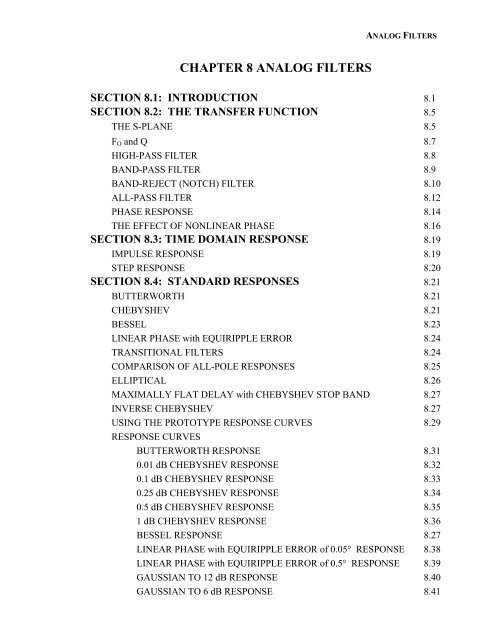
<strong>CHAPTER</strong> 8 <strong>ANALOG</strong> <strong>FILTERS</strong><br />
<strong>ANALOG</strong> <strong>FILTERS</strong><br />
SECTION 8.1: INTRODUCTION 8.1<br />
SECTION 8.2: THE TRANSFER FUNCTION 8.5<br />
THE S-PLANE 8.5<br />
FO and Q 8.7<br />
HIGH-PASS FILTER 8.8<br />
BAND-PASS FILTER 8.9<br />
BAND-REJECT (NOTCH) FILTER 8.10<br />
ALL-PASS FILTER 8.12<br />
PHASE RESPONSE 8.14<br />
THE EFFECT OF NONLINEAR PHASE 8.16<br />
SECTION 8.3: TIME DOMAIN RESPONSE 8.19<br />
IMPULSE RESPONSE 8.19<br />
STEP RESPONSE 8.20<br />
SECTION 8.4: STANDARD RESPONSES 8.21<br />
BUTTERWORTH 8.21<br />
CHEBYSHEV 8.21<br />
BESSEL 8.23<br />
LINEAR PHASE with EQUIRIPPLE ERROR 8.24<br />
TRANSITIONAL <strong>FILTERS</strong> 8.24<br />
COMPARISON OF ALL-POLE RESPONSES 8.25<br />
ELLIPTICAL 8.26<br />
MAXIMALLY FLAT DELAY with CHEBYSHEV STOP BAND 8.27<br />
INVERSE CHEBYSHEV 8.27<br />
USING THE PROTOTYPE RESPONSE CURVES 8.29<br />
RESPONSE CURVES<br />
BUTTERWORTH RESPONSE 8.31<br />
0.01 dB CHEBYSHEV RESPONSE 8.32<br />
0.1 dB CHEBYSHEV RESPONSE 8.33<br />
0.25 dB CHEBYSHEV RESPONSE 8.34<br />
0.5 dB CHEBYSHEV RESPONSE 8.35<br />
1 dB CHEBYSHEV RESPONSE 8.36<br />
BESSEL RESPONSE 8.27<br />
LINEAR PHASE with EQUIRIPPLE ERROR of 0.05° RESPONSE 8.38<br />
LINEAR PHASE with EQUIRIPPLE ERROR of 0.5° RESPONSE 8.39<br />
GAUSSIAN TO 12 dB RESPONSE 8.40<br />
GAUSSIAN TO 6 dB RESPONSE 8.41
BASIC LINEAR DESIGN<br />
SECTION 8.4: STANDARD RESPONSES (cont.)<br />
DESIGN TABLES<br />
BUTTERWORTH DESIGN TABLE 8.42<br />
0.01 dB CHEBYSHEV DESIGN TABLE 8.43<br />
0.1 dB CHEBYSHEV DESIGN TABLE 8.44<br />
0.25 dB CHEBYSHEV DESIGN TABLE 8.45<br />
0.5 dB CHEBYSHEV DESIGN TABLE 8.46<br />
1 dB CHEBYSHEV DESIGN TABLE 8.47<br />
BESSEL DESIGN TABLE<br />
LINEAR PHASE with EQUIRIPPLE ERROR of 0.05° DESIGN<br />
8.48<br />
TABLE<br />
LINEAR PHASE with EQUIRIPPLE ERROR of 0.5° DESIGN<br />
8.49<br />
TABLE 8.50<br />
GAUSSIAN TO 12 dB DESIGN TABLE 8.51<br />
GAUSSIAN TO 6 dB DESIGN TABLE 8.52<br />
SECTION 8.5: FREQUENCY TRANSFORMATION 8.55<br />
LOW-PASS TO HIGH-PASS 8.55<br />
LOW-PASS TO BAND-PASS 8.56<br />
LOW-PASS TO BAND-REJECT (NOTCH) 8.59<br />
LOW-PASS TO ALL-PASS 8.61<br />
SECTION 8.6: FILTER REALIZATIONS 8.63<br />
SINGLE POLE RC 8.64<br />
PASSIVE LC SECTION 8.65<br />
INTEGRATOR 8.67<br />
GENERAL IMPEDANCE CONVERTER 8.68<br />
ACTIVE INDUCTOR 8.69<br />
FREQUENCY DEPENDENT NEGATIVE RESISTOR (FDNR) 8.70<br />
SALLEN-KEY 8.72<br />
MULTIPLE FEEDBACK 8.75<br />
STATE VARIABLE 8.77<br />
BIQUADRATIC (BIQUAD) 8.79<br />
DUAL AMPLIFIER BAND-PASS (DABP) 8.80<br />
TWIN T NOTCH 8.81<br />
BAINTER NOTCH 8.82<br />
BOCTOR NOTCH 8.83<br />
1 BAND-PASS NOTCH 8.85<br />
FIRST ORDER ALL-PASS 8.86<br />
SECOND ORDER ALL-PASS 8.87
SECTION 8.6: FILTER REALIZATIONS (cont.)<br />
DESIGN PAGES<br />
<strong>ANALOG</strong> <strong>FILTERS</strong><br />
SINGLE-POLE 8.88<br />
SALLEN-KEY LOW-PASS 8.89<br />
SALLEN-KEY HIGH-PASS 8.90<br />
SALLEN-KEY BAND-PASS 8.91<br />
MULTIPLE FEEDBACK LOW-PASS 8.92<br />
MULTIPLE FEEDBACK HIGH-PASS 8.93<br />
MULTIPLE FEEDBACK BAND-PASS 8.94<br />
STATE VARIABLE 8.95<br />
BIQUAD 8.98<br />
DUAL AMPLIFIER BAND-PASS 8.100<br />
TWIN T NOTCH 8.101<br />
BAINTER NOTCH 8.102<br />
BOCTOR NOTCH (LOW-PASS) 8.103<br />
BOCTOR NOTCH (HIGH-PASS) 8.104<br />
FIRST ORDER ALL-PASS 8.106<br />
SECOND ORDER ALL-PASS 8.107<br />
SECTION 8.7: PRACTICAL PROBLEMS IN FILTER<br />
IMPLEMENTATION 8.109<br />
PASSIVE COMPONENTS 8.109<br />
LIMITATIONS OF ACTIVE ELEMENTS (OP AMPS) IN <strong>FILTERS</strong> 8.114<br />
DISTORTION RESULTING FROM INPUT CAPACITANCE<br />
MODULATION 8.115<br />
Q PEAKING AND Q ENHANSEMENT 8.117<br />
SECTION 8.8: DESIGN EXAMPLES 8.121<br />
ANTIALIASING FILTER 8.121<br />
TRANSFORMATIONS 8.128<br />
CD RECONSTRUCTION FILTER 8.134<br />
DIGITALLY PROGRAMMABLE STATE VARIABLE FILTER 8.137<br />
60 HZ. NOTCH FILTER 8.141<br />
REFERENCES 8.143
BASIC LINEAR DESIGN
<strong>CHAPTER</strong> 8: <strong>ANALOG</strong> <strong>FILTERS</strong><br />
SECTION 8.1: INTRODUCTION<br />
<strong>ANALOG</strong> <strong>FILTERS</strong><br />
INTRODUCTION<br />
Filters are networks that process signals in a frequency-dependent manner. The basic<br />
concept of a filter can be explained by examining the frequency dependent nature of the<br />
impedance of capacitors and inductors. Consider a voltage divider where the shunt leg is<br />
a reactive impedance. As the frequency is changed, the value of the reactive impedance<br />
changes, and the voltage divider ratio changes. This mechanism yields the frequency<br />
dependent change in the input/output transfer function that is defined as the frequency<br />
response.<br />
Filters have many practical applications. A simple, single-pole, low-pass filter (the<br />
integrator) is often used to stabilize amplifiers by rolling off the gain at higher<br />
frequencies where excessive phase shift may cause oscillations.<br />
A simple, single-pole, high-pass filter can be used to block dc offset in high gain<br />
amplifiers or single supply circuits. Filters can be used to separate signals, passing those<br />
of interest, and attenuating the unwanted frequencies.<br />
An example of this is a radio receiver, where the signal you wish to process is passed<br />
through, typically with gain, while attenuating the rest of the signals. In data conversion,<br />
filters are also used to eliminate the effects of aliases in A/D systems. They are used in<br />
reconstruction of the signal at the output of a D/A as well, eliminating the higher<br />
frequency components, such as the sampling frequency and its harmonics, thus<br />
smoothing the waveform.<br />
There are a large number of texts dedicated to filter theory. No attempt will be made to<br />
go heavily into much of the underlying math: Laplace transforms, complex conjugate<br />
poles and the like, although they will be mentioned.<br />
While they are appropriate for describing the effects of filters and examining stability, in<br />
most cases examination of the function in the frequency domain is more illuminating.<br />
An ideal filter will have an amplitude response that is unity (or at a fixed gain) for the<br />
frequencies of interest (called the pass band) and zero everywhere else (called the stop<br />
band). The frequency at which the response changes from passband to stopband is<br />
referred to as the cutoff frequency.<br />
Figure 8.1(A) shows an idealized low-pass filter. In this filter the low frequencies are in<br />
the pass band and the higher frequencies are in the stop band.<br />
8.1
8.2<br />
BASIC LINEAR DESIGN<br />
The functional complement to the low-pass filter is the high-pass filter. Here, the low<br />
frequencies are in the stop-band, and the high frequencies are in the pass band.<br />
Figure 8.1(B) shows the idealized high-pass filter.<br />
MAGNITUDE<br />
MAGNITUDE<br />
f c<br />
FREQUENCY<br />
(A) Lowpass (B) Highpass<br />
Figure 8.1: Idealized Filter Responses<br />
FREQUENCY<br />
(C) Bandpass (D) Notch (Bandreject)<br />
If a high-pass filter and a low-pass filter are cascaded, a band pass filter is created. The<br />
band pass filter passes a band of frequencies between a lower cutoff frequency, f l, and an<br />
upper cutoff frequency, f h. Frequencies below f l and above f h are in the stop band. An<br />
idealized band pass filter is shown in Figure 8.1(C).<br />
A complement to the band pass filter is the band-reject, or notch filter. Here, the pass<br />
bands include frequencies below f l and above f h. The band from f l to f h is in the stop<br />
band. Figure 8.1(D) shows a notch response.<br />
The idealized filters defined above, unfortunately, cannot be easily built. The transition<br />
from pass band to stop band will not be instantaneous, but instead there will be a<br />
transition region. Stop band attenuation will not be infinite.<br />
The five parameters of a practical filter are defined in Figure 8.2, opposite.<br />
The cutoff frequency (F c ) is the frequency at which the filter response leaves the error<br />
band (or the −3 dB point for a Butterworth response filter). The stop band frequency (F s )<br />
is the frequency at which the minimum attenuation in the stopband is reached. The pass<br />
band ripple (A max ) is the variation (error band) in the pass band response. The minimum<br />
pass band attenuation (A min ) defines the minimum signal attenuation within the stop<br />
band. The steepness of the filter is defined as the order (M) of the filter. M is also the<br />
number of poles in the transfer function. A pole is a root of the denominator of the<br />
transfer function. Conversely, a zero is a root of the numerator of the transfer function.<br />
MAGNITUDE<br />
MAGNITUDE<br />
f1 fh FREQUENCY f1 fh FREQUENCY<br />
f c
<strong>ANALOG</strong> <strong>FILTERS</strong><br />
INTRODUCTION<br />
Each pole gives a –6 dB/octave or –20 dB/decade response. Each zero gives a<br />
+6 dB/octave, or +20 dB/decade response.<br />
STOPBAND<br />
ATTENUATION<br />
AMIN PASS BAND<br />
TRANSITION<br />
BAND<br />
PASSBAND<br />
RIPPLE<br />
A<br />
MAX<br />
3dB POINT<br />
OR<br />
CUTOFF FREQUENCY<br />
F<br />
c<br />
STOPBAND<br />
FREQUENCY<br />
Fs<br />
STOP BAND<br />
Figure 8.2: Key Filter Parameters<br />
Note that not all filters will have all these features. For instance, all-pole configurations<br />
(i.e. no zeros in the transfer function) will not have ripple in the stop band. Butterworth<br />
and Bessel filters are examples of all-pole filters with no ripple in the pass band.<br />
Typically, one or more of the above parameters will be variable. For instance, if you were<br />
to design an antialiasing filter for an ADC, you will know the cutoff frequency (the<br />
maximum frequency that you want to pass), the stop band frequency, (which will<br />
generally be the Nyquist frequency (= ½ the sample rate)) and the minimum attenuation<br />
required (which will be set by the resolution or dynamic range of the system). You can<br />
then go to a chart or computer program to determine the other parameters, such as filter<br />
order, F0, and Q, which determines the peaking of the section, for the various sections<br />
and/or component values.<br />
It should also be pointed out that the filter will affect the phase of a signal, as well as the<br />
amplitude. For example, a single-pole section will have a 90° phase shift at the crossover<br />
frequency. A pole pair will have a 180° phase shift at the crossover frequency. The Q of<br />
the filter will determine the rate of change of the phase. This will be covered more in<br />
depth in the next section.<br />
8.3
8.4<br />
BASIC LINEAR DESIGN<br />
Notes:
SECTION 8.2: THE TRANSFER FUNCTION<br />
The S-Plane<br />
<strong>ANALOG</strong> <strong>FILTERS</strong><br />
THE TRANSFER FUNCTION<br />
Filters have a frequency dependent response because the impedance of a capacitor or an<br />
inductor changes with frequency. Therefore the complex impedances:<br />
and<br />
are used to describe the impedance of an inductor and a capacitor, respectively,<br />
where σ is the Neper frequency in nepers per second (NP/s) and ω is the angular<br />
frequency in radians per sec (rad/s).<br />
By using standard circuit analysis techniques, the transfer equation of the filter can be<br />
developed. These techniques include Ohm’s law, Kirchoff’s voltage and current laws,<br />
and superposition, remembering that the impedances are complex. The transfer equation<br />
is then:<br />
H(s) =<br />
a ms m + a m-1s m-1 + … + a 1s + a 0<br />
b ns n + b n-1s n-1 + … + b 1s + b 0<br />
Therefore, H(s) is a rational function of s with real coefficients with the degree of m for<br />
the numerator and n for the denominator. The degree of the denominator is the order of<br />
the filter. Solving for the roots of the equation determines the poles (denominator) and<br />
zeros (numerator) of the circuit. Each pole will provide a –6 dB/octave or –20 dB/decade<br />
response. Each zero will provide a +6 dB/octave or +20 dB/decade response. These roots<br />
can be real or complex. When they are complex, they occur in conjugate pairs. These<br />
roots are plotted on the s plane (complex plane) where the horizontal axis is σ (real axis)<br />
and the vertical axis is ω (imaginary axis). How these roots are distributed on the s plane<br />
can tell us many things about the circuit. In order to have stability, all poles must be in<br />
the left side of the plane. If we have a zero at the origin, that is a zero in the numerator,<br />
the filter will have no response at dc (high-pass or band pass).<br />
Assume an RLC circuit, as in Figure 8.3. Using the voltage divider concept it can be<br />
shown that the voltage across the resistor is:<br />
H(s)<br />
= Vo<br />
Vin<br />
Z L = s L<br />
Z C =<br />
1<br />
s C<br />
s = σ + jω<br />
=<br />
RCs<br />
LCs 2 + RCs + 1<br />
Eq. 8-1<br />
Eq. 8-2<br />
Eq. 8-3<br />
Eq. 8-4<br />
Eq. 8-5<br />
8.5
8.6<br />
BASIC LINEAR DESIGN<br />
~<br />
Figure 8.3: RLC Circuit<br />
Substituting the component values into the equation yields:<br />
Factoring the equation and normalizing gives:<br />
H(s) = 10 x 3 H(s) = 10 x 3 H(s) = 10 x 3<br />
10mH 10µF<br />
H(s) = 10 3<br />
[ s - ( -0.5 + j 3.122 ) 10 x<br />
x<br />
3 ] [ s - ( -0.5 - j 3.122 ) 103 [ s - ( -0.5 + j 3.122 ) x10<br />
x<br />
x ]<br />
3 ] [ s - ( -0.5 - j 3.122 ) 103 x<br />
]<br />
–0.5<br />
X<br />
X<br />
x<br />
Im (krad / s)<br />
10Ω<br />
Figure 8.4: Pole and Zero Plotted on the s-Plane<br />
s<br />
s 2 + 10 3 s + 10 7<br />
s<br />
+3.122<br />
–3.122<br />
V OUT<br />
Re (kNP / s)<br />
Eq. 8-6<br />
Eq 8-7
This gives a zero at the origin and a pole pair at:<br />
Next, plot these points on the s plane as shown in Figure 8.4:<br />
<strong>ANALOG</strong> <strong>FILTERS</strong><br />
THE TRANSFER FUNCTION<br />
The above discussion has a definite mathematical flavor. In most cases we are more<br />
interested in the circuit’s performance in real applications. While working in the s plane<br />
is completely valid, I’m sure that most of us don’t think in terms of Nepers and imaginary<br />
frequencies.<br />
Fo and Q<br />
s = (-0.5 ± j3.122) x 10 3<br />
So if it is not convenient to work in the s plane, why go through the above discussion?<br />
The answer is that the groundwork has been set for two concepts that will be infinitely<br />
more useful in practice: Fo and Q.<br />
Fo is the cutoff frequency of the filter. This is defined, in general, as the frequency where<br />
the response is down 3 dB from the pass band. It can sometimes be defined as the<br />
frequency at which it will fall out of the pass band. For example, a 0.1 dB Chebyshev<br />
filter can have its Fo at the frequency at which the response is down > 0.1 dB.<br />
The shape of the attenuation curve (as well as the phase and delay curves, which define<br />
the time domain response of the filter) will be the same if the ratio of the actual frequency<br />
to the cutoff frequency is examined, rather than just the actual frequency itself.<br />
Normalizing the filter to 1 rad/s, a simple system for designing and comparing filters can<br />
be developed. The filter is then scaled by the cutoff frequency to determine the<br />
component values for the actual filter.<br />
Q is the “quality factor” of the filter. It is also sometimes given as α where:<br />
α =<br />
This is commonly known as the damping ratio. ξ is sometimes used where:<br />
1<br />
Q<br />
ξ = 2 α<br />
Eq. 8-8<br />
Eq. 8-9<br />
Eq. 8-10<br />
If Q is > 0.707, there will be some peaking in the filter response. If the Q is < 0.707,<br />
rolloff at F0 will be greater; it will have a more gentle slope and will begin sooner. The<br />
amount of peaking for a 2 pole low-pass filter vs. Q is shown in Figure 8.5.<br />
8.7
8.8<br />
BASIC LINEAR DESIGN<br />
MAGNITUDE (dB)<br />
30<br />
20<br />
10<br />
0<br />
–10<br />
–20<br />
–30<br />
–40<br />
–50<br />
Figure 8.5: Low-Pass Filter Peaking vs. Q<br />
Rewriting the transfer function H(s) in terms of ωo and Q:<br />
where Ho is the pass-band gain and ωo = 2π Fo.<br />
This is now the low-pass prototype that will be used to design the filters.<br />
High-Pass Filter<br />
H(s) =<br />
Changing the numerator of the transfer equation, H(s), of the low-pass prototype to H0s 2<br />
transforms the low-pass filter into a high-pass filter. The response of the high-pass filter<br />
is similar in shape to a low-pass, just inverted in frequency.<br />
The transfer function of a high-pass filter is then:<br />
H(s) =<br />
s 2 +<br />
Q = 20<br />
Q = 0.1<br />
0.1 1 10<br />
FREQUENCY (Hz)<br />
H 0 s 2<br />
s 2 + ω 0<br />
Q s<br />
+ ω 0 2<br />
+ ω 0 2<br />
The response of a 2-pole high-pass filter is illustrated in Figure 8.6.<br />
H 0<br />
ω 0<br />
Q s<br />
Eq. 8-11<br />
Eq. 8-12
MAGNITUDE (dB)<br />
30<br />
20<br />
10<br />
Band-Pass Filter<br />
0<br />
–10<br />
–20<br />
–30<br />
–40<br />
–50<br />
Figure 8.6: High- Pass Filter Peaking vs. Q<br />
<strong>ANALOG</strong> <strong>FILTERS</strong><br />
THE TRANSFER FUNCTION<br />
Changing the numerator of the lowpass prototype to Hoωo 2 will convert the filter to a<br />
band-pass function.<br />
The transfer function of a band-pass filter is then:<br />
H(s) =<br />
ωo here is the frequency (F0 = 2 π ω0) at which the gain of the filter peaks.<br />
Ho is the circuit gain and is defined:<br />
FREQUENCY (Hz)<br />
s2 s + 2 +<br />
H H0ω 2<br />
0ω 2<br />
0<br />
Ho = H/Q.<br />
Q has a particular meaning for the band-pass response. It is the selectivity of the filter. It<br />
is defined as:<br />
Q =<br />
FH - FL Eq. 8-15<br />
where FL and FH are the frequencies where the response is –3 dB from the maximum.<br />
The bandwidth (BW) of the filter is described as:<br />
It can be shown that the resonant frequency (F0) is the geometric mean of FL and FH,<br />
BW = FH - F Eq. 8-16<br />
L<br />
ω 0<br />
Q s<br />
Q s<br />
Q s<br />
F 0<br />
Q = 20<br />
Q = 0.1<br />
0.1 1 10<br />
+ ω 2<br />
0<br />
Eq. 8-13<br />
Eq. 8-14<br />
8.9
8.10<br />
BASIC LINEAR DESIGN<br />
which means that F0 will appear half way between FL and FH on a logarithmic scale.<br />
Also, note that the skirts of the band-pass response will always be symmetrical around F0<br />
on a logarithmic scale.<br />
The response of a band-pass filter to various values of Q are shown in Figure 8.7.<br />
A word of caution is appropriate here. Band-pass filters can be defined two different<br />
ways. The narrow-band case is the classic definition that we have shown above.<br />
In some cases, however, if the high and low cutoff frequencies are widely separated, the<br />
band-pass filter is constructed out of separate high-pass and low-pass sections. Widely<br />
separated in this context means separated by at least 2 octaves (× 4 in frequency). This is<br />
the wideband case.<br />
MAGNITUDE (dB)<br />
10<br />
0<br />
–10<br />
–20<br />
–30<br />
–40<br />
–50<br />
–60<br />
Band-Reject (Notch) Filter<br />
F 0 = √F H F L<br />
Q = 100<br />
Q = 0.1<br />
–70<br />
0.1 1 10<br />
FREQUENCY (Hz)<br />
Figure 8.7: Band-Pass Filter Peaking vs. Q<br />
By changing the numerator to s 2 + ωz 2 , we convert the filter to a band-reject or notch<br />
filter. As in the bandpass case, if the corner frequencies of the band-reject filter are<br />
separated by more than an octave (the wideband case), it can be built out of separate lowpass<br />
and high-pass sections. We will adopt the following convention: A narrow-band<br />
band-reject filter will be referred to as a notch filter and the wideband band-reject filter<br />
will be referred to as band-reject filter.<br />
Eq. 8-17
A notch (or band-reject) transfer function is:<br />
<strong>ANALOG</strong> <strong>FILTERS</strong><br />
THE TRANSFER FUNCTION<br />
There are three cases of the notch filter characteristics. These are illustrated in Figure 8.8<br />
(opposite). The relationship of the pole frequency, ω0, and the zero frequency, ωz,<br />
determines if the filter is a standard notch, a lowpass notch or a highpass notch.<br />
If the zero frequency is equal to the pole frequency a standard notch exists. In this<br />
instance the zero lies on the jω plane where the curve that defines the pole frequency<br />
intersects the axis.<br />
A lowpass notch occurs when the zero frequency is greater than the pole frequency. In<br />
this case ωz lies outside the curve of the pole frequencies. What this means in a practical<br />
sense is that the filter's response below ωz will be greater than the response above ωz.<br />
This results in an elliptical low-pass filter.<br />
AMPLITUDE (dB)<br />
LOWPASS NOTCH<br />
STANDARD NOTCH<br />
HIGHPASS NOTCH<br />
H(s) =<br />
H0 ( s 2 + ωz 2 )<br />
s 2 + ω0<br />
Q s<br />
FREQUENCY (kHz)<br />
+ ω0 2<br />
0.1 0.3 1.0 3.0 10<br />
Figure 8.8: Standard, Lowpass, and Highpass Notches<br />
Eq. 8-18<br />
A high-pass notch filter occurs when the zero frequency is less than the pole frequency.<br />
In this case ωz lies inside the curve of the pole frequencies. What this means in a<br />
practical sense is that the filters response below ωz will be less than the response above<br />
ωz . This results in an elliptical high-pass filter.<br />
8.11
8.12<br />
BASIC LINEAR DESIGN<br />
MAGNITUDE (dB)<br />
Figure 8.9: Notch Filter Width versus Frequency for Various Q Values<br />
The variation of the notch width with Q is shown in Figure 8.9.<br />
All-pass Filter<br />
5<br />
0<br />
–5<br />
–10<br />
–15<br />
–20<br />
–25<br />
–30<br />
–35<br />
–40<br />
–45<br />
–50<br />
There is another type of filter that leaves the amplitude of the signal intact but introduces<br />
phase shift. This type of filter is called an all-pass. The purpose of this filter is to add<br />
phase shift (delay) to the response of the circuit. The amplitude of an all-pass is unity for<br />
all frequencies. The phase response, however, changes from 0° to 360° as the frequency<br />
is swept from 0 to infinity. The purpose of an all-pass filter is to provide phase<br />
equalization, typically in pulse circuits. It also has application in single side band,<br />
suppressed carrier (SSB-SC) modulation circuits.<br />
The transfer function of an all-pass filter is:<br />
H(s) =<br />
Q = 20<br />
FREQUENCY (Hz)<br />
s 2 - ω 0<br />
Q s<br />
s 2 + ω 0<br />
Q s<br />
Note that an all-pass transfer function can be synthesized as:<br />
HAP = HLP – HBP + HHP = 1 – 2HBP.<br />
Figure 8.10 (opposite) compares the various filter types.<br />
Q = 0.1<br />
0.1 1 10<br />
+ ω 0 2<br />
+ ω 0 2<br />
Eq. 8-19<br />
Eq. 8-20
FILTER<br />
TYPE<br />
LOWPASS<br />
BANDPASS<br />
NOTCH<br />
(BANDREJECT)<br />
HIGHPASS<br />
MAGNITUDE<br />
Figure 8.10: Standard Second-order Filter Responses<br />
XX<br />
XX<br />
XX<br />
XX<br />
XX<br />
XX<br />
XX<br />
XX<br />
XX<br />
XX<br />
<strong>ANALOG</strong> <strong>FILTERS</strong><br />
THE TRANSFER FUNCTION<br />
POLE LOCATION TRANSFER<br />
EQUATION<br />
ω 2<br />
0<br />
ω0 s2 + s + ω 2<br />
o<br />
Q<br />
s2 ω0 Q<br />
ω<br />
+ 0s<br />
+ ω 2<br />
o<br />
Q<br />
s<br />
s2 s<br />
ω<br />
+ 0s<br />
+ ω 2<br />
o<br />
Q<br />
2 + ω 2<br />
z<br />
s2 ω<br />
+ 0s<br />
+ ω 2<br />
o Q<br />
ALLPASS ω<br />
s 0 2 s<br />
+ s + ω 2<br />
o Q<br />
2 ω0 - s + ω 2<br />
o<br />
Q<br />
s 2<br />
8.13
8.14<br />
BASIC LINEAR DESIGN<br />
Phase Response<br />
As mentioned earlier, a filter will change the phase of the signal as well as the amplitude.<br />
The question is, does this make a difference? Fourier analysis indicates a square wave is<br />
made up of a fundamental frequency and odd order harmonics. The magnitude and phase<br />
responses, of the various harmonics, are precisely defined. If the magnitude or phase<br />
relationships are changed, then the summation of the harmonics will not add back<br />
together properly to give a square wave. It will instead be distorted, typically showing<br />
overshoot and ringing or a slow rise time. This would also hold for any complex<br />
waveform.<br />
Each pole of a filter will add 45° of phase shift at the corner frequency. The phase will<br />
vary from 0° (well below the corner frequency) to 90° (well beyond the corner<br />
frequency). The start of the change can be more than a decade away. In multipole filters,<br />
each of the poles will add phase shift, so that the total phase shift will be multiplied by<br />
the number of poles (180° total shift for a two pole system, 270° for a three pole system,<br />
etc.).<br />
The phase response of a single-pole, low-pass filter is:<br />
φ (ω) = -arctan ω<br />
φ (ω) = -arctan ω<br />
The phase response of a low-pass pole pair is:<br />
+ √ 4 - α2 1 ω<br />
- arctan[<br />
α ( 2<br />
ω ) ]<br />
o<br />
- √ 4 - α2 φ (ω) =<br />
1 ω<br />
- arctan[<br />
α ( 2 ) ]<br />
For a single-pole, high-pass filter the phase response is:<br />
φ (ω) =<br />
π<br />
2<br />
ω o<br />
- arctan ω<br />
ω o<br />
The phase response of a high-pass pole pair is:<br />
φ (ω) =<br />
+ √ 4 - α2 1<br />
- arctan[<br />
α ( 2<br />
ω<br />
ωo ) ]<br />
- √ 4 - α2 π<br />
- arctan<br />
1<br />
α ( 2<br />
ω<br />
)<br />
ω o<br />
[ ]<br />
ω o<br />
Eq. 8-21<br />
Eq. 8-22<br />
Eq. 8-23<br />
Eq. 8-24
The phase response of a band-pass filter is:<br />
φ (ω) =<br />
π<br />
2<br />
- arctan<br />
- arctan<br />
(<br />
+ √4Q2 2Qω<br />
ω0 - 1<br />
- √4Q2 2Qω<br />
ω0 - 1 )<br />
<strong>ANALOG</strong> <strong>FILTERS</strong><br />
THE TRANSFER FUNCTION<br />
The variation of the phase shift with frequency due to various values of Q is shown in<br />
Figure 8.11 (for low-pass, high-pass, band-pass, and all-pass) and in Figure 8.12 (for<br />
notch).<br />
PHASE (DEGREES)<br />
0<br />
180<br />
–40 160<br />
–80 140<br />
90<br />
70<br />
50<br />
0<br />
–20<br />
–40<br />
–120 120 30 –60<br />
–160 100<br />
–200<br />
–240<br />
–280<br />
–320<br />
–360<br />
ALLPASS<br />
10<br />
–80<br />
80 –10 –100<br />
60 –30 –120<br />
40 –50 –140<br />
20 –70 –160<br />
0<br />
BANDPASS<br />
Figure 8.11: Phase Response vs. Frequency<br />
(<br />
–90 –180<br />
0.1 1 10<br />
HIGHPASS<br />
LOWPASS<br />
Q = 0.1<br />
Q = 20<br />
Q = 20<br />
FREQUENCY (Hz)<br />
)<br />
Q = 0.1<br />
Eq. 8-25<br />
8.15
8.16<br />
BASIC LINEAR DESIGN<br />
Figure 8.12: Notch Filter Phase Response<br />
It is also useful to look at the change of phase with frequency. This is the group delay of<br />
the filter. A flat (constant) group delay gives best phase response, but, unfortunately, it<br />
also gives the least amplitude discrimination. The group delay of a single low-pass pole<br />
is:<br />
PHASE (DEGREES)<br />
For the low-pass pole pair it is:<br />
For the single high-pass pole it is:<br />
For the high-pass pole pair it is:<br />
90<br />
70<br />
50<br />
30<br />
10<br />
–10<br />
–30<br />
–50<br />
–70<br />
Q=0.1<br />
–90<br />
0.1 1 10<br />
And for the band-pass pole pair it is:<br />
τ (ω) = = cos2 dφ (ω) φ<br />
-<br />
dω<br />
τ (ω) = 2 sin2 φ<br />
αω 0<br />
τ (ω) = 2 sin2 φ<br />
αω 0<br />
-<br />
ω 0<br />
sin 2 φ<br />
2 ω<br />
sin 2 φ<br />
2 ω<br />
τ(ω) = = sin2 dφ (ω) φ<br />
-<br />
dω<br />
τ (ω) = 2Q 2 cos2 φ<br />
τ (ω) = +<br />
2Q 2 cos2 φ<br />
+<br />
αω 0<br />
Q=20<br />
-<br />
FREQUENCY (Hz)<br />
ω 0<br />
sin 2 φ<br />
2 ω<br />
Q=0.1<br />
Q=20<br />
Eq. 8-26<br />
Eq. 8-27<br />
Eq. 8-28<br />
Eq. 8-29<br />
Eq. 8-30
The Effect of Nonlinear Phase<br />
<strong>ANALOG</strong> <strong>FILTERS</strong><br />
THE TRANSFER FUNCTION<br />
A waveform can be represented by a series of frequencies of specific amplitude,<br />
frequency and phase relationships. For example, a square wave is:<br />
1 2 2<br />
2<br />
2<br />
Eq. 8-31<br />
F(t) = A( 2 + π sin ω t + sin 3ω t + sin 5ω t + sin 7ω t + ….)<br />
3 π 5 π 7 π<br />
If this waveform were passed through a filter, the amplitude and phase response of the<br />
filter to the various frequency components of the waveform could be different. If the<br />
phase delays were identical, the waveform would pass through the filter undistorted. If,<br />
however, the different components of the waveform were changed due to different<br />
amplitude and phase response of the filter to those frequencies, they would no longer add<br />
up in the same manner. This would change the shape of the waveform. These distortions<br />
would manifest themselves in what we typically call overshoot and ringing of the output.<br />
Not all signals will be composed of harmonically related components. An amplitude<br />
modulated (AM) signal, for instance, will consist of a carrier and 2 sidebands at ± the<br />
modulation frequency. If the filter does not have the same delay for the various waveform<br />
components, then “envelope delay” will occur and the output wave will be distorted.<br />
Linear phase shift results in constant group delay since the derivative of a linear function<br />
is a constant.<br />
8.17
8.18<br />
BASIC LINEAR DESIGN<br />
Notes:
SECTION 8.3: TIME DOMAIN RESPONSE<br />
<strong>ANALOG</strong> <strong>FILTERS</strong><br />
TIME DOMAIN RESPONSES<br />
Up until now the discussion has been primarily focused on the frequency domain<br />
response of filters. The time domain response can also be of concern, particularly under<br />
transient conditions. Moving between the time domain and the frequency domain is<br />
accomplished by the use of the Fourier and Laplace transforms. This yields a method of<br />
evaluating performance of the filter to a nonsinusoidal excitation.<br />
The transfer function of a filter is the ratio of the output to input time functions. It can be<br />
shown that the impulse response of a filter defines its bandwidth. The time domain<br />
response is a practical consideration in many systems, particularly communications,<br />
where many modulation schemes use both amplitude and phase information.<br />
Impulse Response<br />
The impulse function is defined as an infinitely high, infinitely narrow pulse, with an area<br />
of unity. This is, of course, impossible to realize in a physical sense. If the impulse width<br />
is much less than the rise time of the filter, the resulting response of the filter will give a<br />
reasonable approximation actual impulse response of the filter response.<br />
The impulse response of a filter, in the time domain, is proportional to the bandwidth of<br />
the filter in the frequency domain. The narrower the impulse, the wider the bandwidth of<br />
the filter. The pulse amplitude is equal to ωc/π, which is also proportional to the filter<br />
bandwidth, the height being taller for wider bandwidths. The pulse width is equal to<br />
2π/ωc, which is inversely proportional to bandwidth. It turns out that the product of the<br />
amplitude and the bandwidth is a constant.<br />
It would be a nontrivial task to calculate the response of a filter without the use of<br />
Laplace and Fourier transforms. The Laplace transform converts multiplication and<br />
division to addition and subtraction, respectively. This takes equations, which are<br />
typically loaded with integration and/or differentiation, and turns them into simple<br />
algebraic equations, which are much easier to deal with. The Fourier transform works in<br />
the opposite direction.<br />
The details of these transform will not be discussed here. However, some general<br />
observations on the relationship of the impulse response to the filter characteristics will<br />
be made.<br />
It can be shown, as stated, that the impulse response is related to the bandwidth.<br />
Therefore, amplitude discrimination (the ability to distinguish between the desired signal<br />
from other, out of band signals and noise) and time response are inversely proportional.<br />
That is to say that the filters with the best amplitude response are the ones with the worst<br />
time response. For all-pole filters, the Chebyshev filter gives the best amplitude<br />
discrimination, followed by the Butterworth and then the Bessel.<br />
8.19
8.20<br />
BASIC LINEAR DESIGN<br />
If the time domain response were ranked, the Bessel would be best, followed by the<br />
Butterworth and then the Chebyshev. Details of the different filter responses will be<br />
discussed in the next section.<br />
The impulse response also increases with increasing filter order. Higher filter order<br />
implies greater bandlimiting, therefore degraded time response. Each section of a<br />
multistage filter will have its own impulse response, and the total impulse response is the<br />
accumulation of the individual responses. The degradation in the time response can also<br />
be related to the fact that as frequency discrimination is increased, the Q of the individual<br />
sections tends to increase. The increase in Q increases the overshoot and ringing of the<br />
individual sections, which implies longer time response.<br />
Step Response<br />
The step response of a filter is the integral of the impulse response. Many of the<br />
generalities that apply to the impulse response also apply to the step response. The slope<br />
of the rise time of the step response is equal to the peak response of the impulse. The<br />
product of the bandwidth of the filter and the rise time is a constant. Just as the impulse<br />
has a function equal to unity, the step response has a function equal to 1/s. Both of these<br />
expressions can be normalized, since they are dimensionless.<br />
The step response of a filter is useful in determining the envelope distortion of a<br />
modulated signal. The two most important parameters of a filter's step response are the<br />
overshoot and ringing. Overshoot should be minimal for good pulse response. Ringing<br />
should decay as fast as possible, so as not to interfere with subsequent pulses.<br />
Real life signals typically aren’t made up of impulse pulses or steps, so the transient<br />
response curves don’t give a completely accurate estimation of the output. They are,<br />
however, a convenient figure of merit so that the transient responses of the various filter<br />
types can be compared on an equal footing.<br />
Since the calculations of the step and impulse response are mathematically intensive,<br />
they are most easily performed by computer. Many CAD (Computer Aided Design)<br />
software packages have the ability to calculate these responses. Several of these<br />
responses are also collected in the next section.
SECTION 8.4: STANDARD RESPONSES<br />
<strong>ANALOG</strong> <strong>FILTERS</strong><br />
STANDARD RESPONSES<br />
There are many transfer functions that may satisfy the attenuation and/or phase<br />
requirements of a particular filter. The one that you choose will depend on the particular<br />
system. The importance of the frequency domain response versus the time domain<br />
response must be determined. Also, both of these considerations might be traded off<br />
against filter complexity, and thereby cost.<br />
Butterworth<br />
The Butterworth filter is the best compromise between attenuation and phase response. It<br />
has no ripple in the pass band or the stop band, and because of this is sometimes called a<br />
maximally flat filter. The Butterworth filter achieves its flatness at the expense of a<br />
relatively wide transition region from pass band to stop band, with average transient<br />
characteristics.<br />
The normalized poles of the Butterworth filter fall on the unit circle (in the s plane). The<br />
pole positions are given by:<br />
where K is the pole pair number, and n is the number of poles.<br />
The poles are spaced equidistant on the unit circle, which means the angles between the<br />
poles are equal.<br />
Given the pole locations, ω0, and α (or Q) can be determined. These values can then be<br />
use to determine the component values of the filter. The design tables for passive filters<br />
use frequency and impedance normalized filters. They are normalized to a frequency of 1<br />
rad/sec and impedance of 1 Ω. These filters can be denormalized to determine actual<br />
component values. This allows the comparison of the frequency domain and/or time<br />
domain responses of the various filters on equal footing. The Butterworth filter is<br />
normalized for a –3 dB response at ωo = 1.<br />
The values of the elements of the Butterworth filter are more practical and less critical<br />
than many other filter types. The frequency response, group delay, impulse response, and<br />
step response are shown in Figure 8.15. The pole locations and corresponding ωo and α<br />
terms are tabulated in Figure 8.26.<br />
Chebyshev<br />
(2K-1)π (2K-1)π<br />
-sin + j cos K=1,2....n Eq. 8-32<br />
2n<br />
2n<br />
The Chebyshev (or Chevyshev, Tschebychev, Tschebyscheff or Tchevysheff, depending<br />
on how you translate from Russian) filter has a smaller transition region than the sameorder<br />
Butterworth filter, at the expense of ripples in its pass band. This filter gets its name<br />
8.21
8.22<br />
BASIC LINEAR DESIGN<br />
because the Chebyshev filter minimizes the height of the maximum ripple, which is the<br />
Chebyshev criterion.<br />
Chebyshev filters have 0 dB relative attenuation at dc. Odd order filters have an<br />
attenuation band that extends from 0 dB to the ripple value. Even order filters have a gain<br />
equal to the pass band ripple. The number of cycles of ripple in the pass band is equal to<br />
the order of the filter.<br />
The poles of the Chebyshev filter can be determined by moving the poles of the<br />
Butterworth filter to the right, forming an ellipse. This is accomplished by multiplying<br />
the real part of the pole by kr and the imaginary part by kI. The values kr and k I can be<br />
computed by:<br />
where:<br />
where n is the filter order and:<br />
where:<br />
where:<br />
K r = sinh A<br />
KI = cosh A<br />
RdB = pass band ripple in dB<br />
The Chebyshev filters are typically normalized so that the edge of the ripple band is at<br />
ωo = 1. The 3 dB bandwidth is given by:<br />
This is tabulated in Table 1.<br />
A = sinh-1 1<br />
n<br />
ε = √ 10 R -1<br />
R =<br />
The frequency response, group delay, impulse response and step response are cataloged<br />
in Figures 8.16 to 8.20 on following pages, for various values of pass band ripple (0 .01<br />
dB, 0.1 dB, 0.25 dB, 0.5 dB, and 1 dB). The pole locations and corresponding ωo and α<br />
terms for these values of ripple are tabulated in Figures 8.27 to 8.31 on following pages.<br />
R dB<br />
10<br />
1<br />
ε<br />
A3dB = cosh-1 1<br />
n<br />
( )<br />
1<br />
ε<br />
Eq. 8-33<br />
Eq. 8-34<br />
Eq. 8-35<br />
Eq. 8-36<br />
Eq. 8-37<br />
Eq. 8-38<br />
Eq. 8-39
<strong>ANALOG</strong> <strong>FILTERS</strong><br />
STANDARD RESPONSES<br />
Table 1: 3dB Bandwidth to Ripple Bandwidth for Chebyshev Filters<br />
Bessel<br />
ORDER .01dB .1dB .25dB .5dB 1dB<br />
2 3.30362 1.93432 1.59814 1.38974 1.21763<br />
3 1.87718 1.38899 1.25289 1.16749 1.09487<br />
4 1.46690 1.21310 1.13977 1.09310 1.05300<br />
5 1.29122 1.13472 1.08872 1.05926 1.03381<br />
6 1.19941 1.09293 1.06134 1.04103 1.02344<br />
7 1.14527 1.06800 1.04495 1.03009 1.01721<br />
8 1.11061 1.05193 1.03435 1.02301 1.01316<br />
9 1.08706 1.04095 1.02711 1.01817 1.01040<br />
10 1.07033 1.03313 1.02194 1.01471 1.00842<br />
Butterworth filters have fairly good amplitude and transient behavior. The Chebyshev<br />
filters improve on the amplitude response at the expense of transient behavior. The<br />
Bessel filter is optimized to obtain better transient response due to a linear phase (i.e.<br />
constant delay) in the passband. This means that there will be relatively poorer frequency<br />
response (less amplitude discrimination).<br />
The poles of the Bessel filter can be determined by locating all of the poles on a circle<br />
and separating their imaginary parts by:<br />
where n is the number of poles. Note that the top and bottom poles are distanced by<br />
where the circle crosses the jω axis by:<br />
1<br />
Eq. 8-41<br />
n<br />
or half the distance between the other poles.<br />
2<br />
n<br />
Eq. 8-40<br />
The frequency response, group delay, impulse response and step response for the Bessel<br />
filters are cataloged in Figure 8.21. The pole locations and corresponding ωo and α terms<br />
for the Bessel filter are tabulated in Figure 8.32.<br />
8.23
8.24<br />
BASIC LINEAR DESIGN<br />
Linear Phase with Equiripple Error<br />
The linear phase filter offers linear phase response in the pass band, over a wider range<br />
than the Bessel, and superior attenuation far from cutoff. This is accomplished by letting<br />
the phase response have ripples, similar to the amplitude ripples of the Chebyshev. As the<br />
ripple is increased, the region of constant delay extends further into the stopband. This<br />
will also cause the group delay to develop ripples, since it is the derivative of the phase<br />
response. The step response will show slightly more overshoot than the Bessel and the<br />
impulse response will show a bit more ringing.<br />
It is difficult to compute the pole locations of a linear phase filter. Pole locations are<br />
taken from the Williams book (see Reference 2), which, in turn, comes from the Zverev<br />
book (see Reference 1).<br />
The frequency response, group delay, impulse response and step response for linear<br />
phase filters of 0.05° ripple and 0.5° ripple are given in Figures 8.22 and 8.23. The pole<br />
locations and corresponding ωo and α terms are tabulated in Figures 8.33 and 8.34.<br />
Transitional Filters<br />
A transitional filter is a compromise between a Gaussian filter, which is similar to a<br />
Bessel, and the Chebyshev. A transitional filter has nearly linear phase shift and smooth,<br />
monotonic rolloff in the pass band. Above the pass band there is a break point beyond<br />
which the attenuation increases dramatically compared to the Bessel, and especially at<br />
higher values of n.<br />
Two transition filters have been tabulated. These are the Gaussian to 6 dB and Gaussian<br />
to 12 dB.<br />
The Gaussian to 6 dB filter has better transient response than the Butterworth in the pass<br />
band. Beyond the breakpoint, which occurs at ω = 1.5, the rolloff is similar to the<br />
Butterworth.<br />
The Gaussian to 12 dB filter’s transient response is much better than Butterworth in the<br />
pass band. Beyond the 12dB breakpoint, which occurs at ω = 2, the attenuation is less<br />
than the Butterworth.<br />
As is the case with the linear phase filters, pole locations for transitional filters do not<br />
have a closed form method for computation. Again, pole locations are taken from<br />
Williams's book (see Reference 2). These were derived from iterative techniques.<br />
The frequency response, group delay, impulse response and step response for Gaussian to<br />
12 dB and 6 dB are shown in Figures 8.24 and 8.25. The pole locations and<br />
corresponding ωo and α terms are tabulated in Figures 8.35 and 8.36.
Comparison of All-Pole Responses<br />
<strong>ANALOG</strong> <strong>FILTERS</strong><br />
STANDARD RESPONSES<br />
The responses of several all-pole filters, namely the Bessel, Butterworth, and Chebyshev<br />
(in this case of 0.5 dB ripple) will now be compared. An 8 pole filter is used as the basis<br />
for the comparison. The responses have been normalized for a cutoff of 1 Hz. Comparing<br />
Figures 8.13 and 8.14 below, it is easy to see the trade-offs in the response types. Moving<br />
from Bessel through Butterworth to Chebyshev, notice that the amplitude discrimination<br />
improves as the transient behavior gets progressively poorer.<br />
Figure 8.13: Comparison of Amplitude Response of<br />
Bessel, Butterworth, and Chebyshev Filters<br />
Figure 8.14: Comparison of Step and Impulse Responses<br />
of Bessel, Butterworth, and Chebyshev Filters<br />
8.25
8.26<br />
BASIC LINEAR DESIGN<br />
Elliptical<br />
The previously mentioned filters are all-pole designs, which mean that the zeros of the<br />
transfer function (roots of the numerator) are at one of the two extremes of the frequency<br />
range (0 or ∞). For a low-pass filter, the zeros are at f = ∞. If finite frequency transfer<br />
function zeros are added to poles an Elliptical filter (sometimes referred to as Cauer<br />
filters) is created. This filter has a shorter transition region than the Chebyshev filter<br />
because it allows ripple in both the stop band and pass band. It is the addition of zeros in<br />
the stop band that causes ripple in the stop band but gives a much higher rate of<br />
attenuation, the most possible for a given number of poles. There will be some<br />
“bounceback” of the stop band response between the zeros. This is the stop band ripple.<br />
The Elliptical filter also has degraded time domain response.<br />
Since the poles of an elliptic filter are on an ellipse, the time response of the filter<br />
resembles that of the Chebyshev.<br />
An Elliptic filter is defined by the parameters shown in Figure 8.2, those being Amax, the<br />
maximum ripple in the passband, Amin, the minimum attenuation in the stopband, Fc, the<br />
cutoff frequency, which is where the frequency response leaves the pass band ripple and<br />
FS, the stopband frequency, where the value of Amax is reached.<br />
An alternate approach is to define a filter order n, the modulation angle, θ, which defines<br />
the rate of attenuation in the transition band, where:<br />
θ = sin-1 θ = sin-1 and ρ which determines the pass band ripple, where:<br />
√ ε2 ε<br />
ρ = √ 2 ε<br />
ρ =<br />
2<br />
ρ =<br />
1 + ε2 1 + ε2 1 + ε2 where ε is the ripple factor developed for the Chebyshev response, and the pass band<br />
ripple is:<br />
RdB = - 10 log (1 - ρ 2 )<br />
Eq. 8-44<br />
Some general observations can be made. For a given filter order n, and θ, Amin increases<br />
as the ripple is made larger. Also, as θ approaches 90°, FS approaches FC. This results in<br />
extremely short transition region, which means sharp rolloff. This comes at the expense<br />
of lower Amin.<br />
As a side note, ρ determines the input resistance of a passive elliptical filter, which can<br />
then be related to the VSWR (Voltage Standing Wave Ratio).<br />
Because of the number of variables in the design of an elliptic filter, it is difficult to<br />
provide the type of tables provided for the previous filter types. Several CAD (Computer<br />
Aided Design) packages can provide the design values. Alternatively several sources,<br />
1<br />
F s<br />
Eq. 8-42<br />
Eq. 8-43
<strong>ANALOG</strong> <strong>FILTERS</strong><br />
STANDARD RESPONSES<br />
such as Williams's (see Reference 2), provide tabulated filter values. These tables classify<br />
the filter by<br />
where the C denotes Cauer. Elliptical filters are sometime referred to as Cauer filters<br />
after the network theorist Wilhelm Cauer.<br />
Maximally Flat Delay with Chebyshev Stop Band<br />
Bessel type (Bessel, linear phase with equiripple error and transitional) filters give<br />
excellent transient behavior, but less than ideal frequency discrimination. Elliptical filters<br />
give better frequency discrimination, but degraded transient response. A maximally flat<br />
delay with Chebyshev stop band filter takes a Bessel type function and adds transmission<br />
zeros. The constant delay properties of the Bessel type filter in the pass band are<br />
maintained, and the stop band attenuation is significantly improved. The step response<br />
exhibits no overshoot or ringing, and the impulse response is clean, with essentially no<br />
oscillatory behavior. Constant group delay properties extend well into the stop band for<br />
increasing n.<br />
As with the elliptical filter, numeric evaluation is difficult. Williams’s book (see<br />
Reference 2) tabulates passive prototypes normalized component values.<br />
Inverse Chebyshev<br />
C n ρ θ<br />
The Chebyshev response has ripple in the pass band and a monotonic stop band. The<br />
inverse Chebyshev response can be defined that has a monotonic pass band and ripple in<br />
the stop band. The inverse Chebyshev has better pass band performance than even the<br />
Butterworth. It is also better than the Chebyshev, except very near the cutoff frequency.<br />
In the transition band, the inverse Chebyshev has the steepest rolloff. Therefore, the<br />
inverse Chebyshev will meet the Amin specification at the lowest frequency of the three.<br />
In the stop band there will, however, be response lobes which have a magnitude of:<br />
ε2 ε2 (1 - ε)<br />
Eq. 8-45<br />
where ε is the ripple factor defined for the Chebyshev case. This means that deep into the<br />
stop band, both the Butterworth and Chebyshev will have better attenuation, since they<br />
are monotonic in the stop band. In terms of transient performance, the inverse Chebyshev<br />
lies midway between the Butterworth and the Chebyshev.<br />
8.27
8.28<br />
BASIC LINEAR DESIGN<br />
The inverse Chebyshev response can be generated in three steps. First take a Chebyshev<br />
low pass filter. Then subtract this response from 1. Finally, invert in frequency by<br />
replacing ω with 1/ω.<br />
These are by no means all the possible transfer functions, but they do represent the most<br />
common.
Using the Prototype Response Curves<br />
<strong>ANALOG</strong> <strong>FILTERS</strong><br />
STANDARD RESPONSES<br />
In the following pages, the response curves and the design tables for several of the low<br />
pass prototypes of the all-pole responses will be cataloged. All the curves are normalized<br />
to a −3 dB cutoff frequency of 1 Hz. This allows direct comparison of the various<br />
responses. In all cases the amplitude response for the 2 through 10 pole cases for the<br />
frequency range of 0.1 Hz. to 10 Hz. will be shown. Then a detail of the amplitude<br />
response in the 0.1 Hz to 2 Hz. pass band will be shown. The group delay from 0.1 Hz to<br />
10 Hz and the impulse response and step response from 0 seconds to 5 seconds will also<br />
be shown.<br />
To use these curves to determine the response of real life filters, they must be<br />
denormalized. In the case of the amplitude responses, this is simply accomplished by<br />
multiplying the frequency axis by the desired cutoff frequency FC. To denormalize the<br />
group delay curves, we divide the delay axis by 2π FC, and multiply the frequency axis<br />
by FC, as before. Denormalize the step response by dividing the time axis by 2π FC.<br />
Denormalize the impulse response by dividing the time axis by 2π FC and multiplying the<br />
amplitude axis by the same amount.<br />
For a high-pass filter, simply invert the frequency axis for the amplitude response. In<br />
transforming a low-pass filter into a high-pass (or band-reject) filter, the transient<br />
behavior is not preserved. Zverev (see Reference 1) provides a computational method for<br />
calculating these responses.<br />
In transforming a lowpass into a narrowband bandpass, the 0Hz axis is moved to the<br />
center frequency F0. It stands to reason that the response of the bandpass case around the<br />
center frequency would then match the lowpass response around 0Hz. The frequency<br />
response curve of a lowpass filter actually mirrors itself around 0Hz, although we<br />
generally don’t concern ourselves with negative frequency.<br />
To denormalize the group delay curve for a bandpass filter, divide the delay axis by<br />
πBW, where BW is the 3dB bandwidth in Hz. Then multiply the frequency axis by<br />
BW/2. In general, the delay of the bandpass filter at F0 will be twice the delay of the<br />
lowpass prototype with the same bandwidth at 0Hz. This is due to the fact that the<br />
lowpass to bandpass transformation results in a filter with order 2n, even though it is<br />
typically referred to it as having the same order as the lowpass filter from which it is<br />
derived. This approximation holds for narrow-band filters. As the bandwidth of the filter<br />
is increased, some distortion of the curve occurs. The delay becomes less symmetrical,<br />
peaking below F0.<br />
The envelope of the response of a band-pass filter resembles the step response of the<br />
lowpass prototype. More exactly, it is almost identical to the step response of a low-pass<br />
filter having half the bandwidth. To determine the envelope response of the band-pass<br />
filter, divide the time axis of the step response of the lowpass prototype by πBW, where<br />
BW is the 3dB bandwidth. The previous discussions of overshoot, ringing, etc. can now<br />
be applied to the carrier envelope.<br />
8.29
8.30<br />
BASIC LINEAR DESIGN<br />
The envelope of the response of a narrow-band band-pass filter to a short burst of carrier<br />
(that is where the burst width is much less than the rise time of the denormalized step<br />
response of the band-pass filter) can be determined by denormalizing the impulse<br />
response of the low-pass prototype. To do this, multiply the amplitude axis and divide the<br />
time axis by πBW, where BW is the 3 dB bandwidth. It is assumed that the carrier<br />
frequency is high enough so that many cycles occur during the burst interval.<br />
While the group delay, step and impulse curves cannot be used directly to predict the<br />
distortion to the waveform caused by the filter, they are a useful figure of merit when<br />
used to compare filters.
AMPLITUDE (dB)<br />
1.0<br />
AMPLITUDE<br />
0<br />
AMPLITUDE<br />
AMPLITUDE (DETAIL) GROUP DELAY<br />
IMPULSE RESPONSE<br />
Figure 8.15: Butterworth Response<br />
<strong>ANALOG</strong> <strong>FILTERS</strong><br />
STANDARD RESPONSES<br />
–4.0<br />
0.1 0.2 0.4 0.8 1.1 2.0<br />
0<br />
0.1 0.4 1.1 4.0 10<br />
FREQUENCY (Hz) FREQUENCY (Hz)<br />
4.0<br />
0<br />
AMPLITUDE (V) 8.0<br />
0<br />
–50<br />
–90<br />
0.1 1.1 10<br />
0.2 0.4 0.8 2.0 4.0 8.0<br />
FREQUENCY (Hz)<br />
AMPLITUDE (V)<br />
STEP RESPONSE<br />
–4.0<br />
0<br />
0 1 2<br />
3 4 5 0 1 2 3 4 5<br />
TIME (s)<br />
TIME (s)<br />
2.0<br />
DELAY (s)<br />
1.0<br />
1.2<br />
0.8<br />
0.4<br />
8.31
AMPLITUDE (dB)<br />
8.32<br />
BASIC LINEAR DESIGN<br />
AMPLITUDE<br />
0<br />
–50<br />
AMPLITUDE<br />
–90<br />
0.1 0.2 0.4 0.8 1.1 2.0 4.0 8.0 10<br />
1.0<br />
0<br />
AMPLITUDE (DETAIL) GROUP DELAY<br />
–4.0<br />
0<br />
0.1 0.2 0.4 0.8 1.1 2.0 0.1 0.4 1.1 4.0 10<br />
FREQUENCY (Hz)<br />
FREQUENCY (Hz)<br />
4.0<br />
0<br />
AMPLITUDE (V) 8.0<br />
IMPULSE RESPONSE<br />
FREQUENCY (Hz)<br />
STEP RESPONSE<br />
–4.0<br />
0<br />
0 1 2<br />
3 4 5 0 1 2 3 4 5<br />
TIME (s)<br />
TIME (s)<br />
Figure 8.16: 0.01 dB Chebyshev Response<br />
AMPLITUDE (V)<br />
DELAY (s)<br />
5.0<br />
1.5<br />
1.0<br />
0.5
AMPLITUDE (dB)<br />
AMPLITUDE<br />
0<br />
–50<br />
AMPLITUDE<br />
Figure 8.17: 0.1 dB Chebyshev Response<br />
<strong>ANALOG</strong> <strong>FILTERS</strong><br />
STANDARD RESPONSES<br />
–90<br />
0.1 0.2 0.4 0.8 1.1 2.0 4.0 8.0 10<br />
1.0<br />
0<br />
AMPLITUDE (DETAIL) GROUP DELAY<br />
IMPULSE RESPONSE<br />
FREQUENCY (Hz)<br />
–4.0<br />
0.1 0.2 0.4 0.8 1.1 2.0<br />
0<br />
0.1 0.4 1.1 4.0 10<br />
FREQUENCY (Hz)<br />
FREQUENCY (Hz)<br />
AMPLITUDE (V)<br />
8.0<br />
4.0<br />
0<br />
–2.0<br />
AMPLITUDE (V)<br />
STEP RESPONSE<br />
0<br />
0 1 2<br />
3 4 5 0 1 2 3 4 5<br />
TIME (s)<br />
TIME (s)<br />
5.0<br />
DELAY (s)<br />
1.5<br />
1.0<br />
0.5<br />
8.33
AMPLITUDE (dB)<br />
8.34<br />
BASIC LINEAR DESIGN<br />
AMPLITUDE<br />
0<br />
–50<br />
AMPLITUDE<br />
–90<br />
0.1 0.2 0.4 0.8 1.1 2.0 4.0 8.0 10<br />
1.0<br />
0<br />
AMPLITUDE (DETAIL) GROUP DELAY<br />
IMPULSE RESPONSE<br />
FREQUENCY (Hz)<br />
–4.0<br />
0.1 0.2 0.4 0.8 1.1 2.0<br />
0<br />
0.1 0.4 1.1 4.0 10<br />
FREQUENCY (Hz)<br />
FREQUENCY (Hz)<br />
4.0<br />
0<br />
AMPLITUDE (V) 8.0<br />
Figure 8.18: 0.25 dB Chebyshev Response<br />
DELAY (s)<br />
AMPLITUDE (V)<br />
1.5<br />
1.0<br />
0.5<br />
STEP RESPONSE<br />
–4.0<br />
0<br />
0 1 2<br />
3 4 5 0 1 2 3 4 5<br />
TIME (s)<br />
TIME (s)<br />
7.0<br />
5.0
AMPLITUDE (V)<br />
AMPLITUDE (dB)<br />
1.0<br />
AMPLITUDE<br />
0<br />
–50<br />
AMPLITUDE<br />
Figure 8.19: 0.5 dB Chebyshev Response<br />
<strong>ANALOG</strong> <strong>FILTERS</strong><br />
STANDARD RESPONSES<br />
–90<br />
0.1 0.2 0.4 0.8 1.1 2.0 4.0 8.0 10<br />
0<br />
AMPLITUDE (DETAIL) GROUP DELAY<br />
IMPULSE RESPONSE<br />
FREQUENCY (Hz)<br />
–4.0<br />
0.1 0.2 0.4 0.8 1.1 2.0<br />
0<br />
0.1 0.4 1.1 4.0 10<br />
FREQUENCY (Hz)<br />
FREQUENCY (Hz)<br />
4.0<br />
2.0<br />
0<br />
–2.0<br />
AMPLITUDE (V)<br />
DELAY (s)<br />
STEP RESPONSE<br />
0<br />
0 1 2<br />
3 4 5 0 1 2 3 4 5<br />
TIME (s)<br />
TIME (s)<br />
6.0<br />
5.0<br />
1.5<br />
1.0<br />
0.5<br />
8.35
AMPLITUDE (dB)<br />
8.36<br />
BASIC LINEAR DESIGN<br />
AMPLITUDE<br />
0<br />
–50<br />
AMPLITUDE<br />
–90<br />
0.1 0.2 0.4 0.8 1.1 2.0 4.0 8.0 10<br />
1.5<br />
0<br />
AMPLITUDE (DETAIL) GROUP DELAY<br />
IMPULSE RESPONSE<br />
FREQUENCY (Hz)<br />
–3.5<br />
0.1 0.2 0.4 0.8 1.1 2.0<br />
0<br />
0.1 0.4 1.1 4.0 10<br />
FREQUENCY (Hz)<br />
FREQUENCY (Hz)<br />
4.0<br />
0<br />
AMPLITUDE (V) 8.0<br />
–4.0<br />
0 1 2<br />
TIME (s)<br />
3 4 5<br />
Figure 8.20: 1 dB Chebyshev Response<br />
AMPLITUDE (V)<br />
8.0<br />
5.0<br />
DELAY (s)<br />
1.5<br />
1.0<br />
0.5<br />
STEP RESPONSE<br />
0<br />
0 1 2<br />
TIME (s)<br />
3 4 5
AMPLITUDE (dB)<br />
0<br />
–50<br />
AMPLITUDE<br />
AMPLITUDE<br />
AMPLITUDE (DETAIL) GROUP DELAY<br />
IMPULSE RESPONSE<br />
FREQUENCY (Hz)<br />
DELAY (s)<br />
Figure 8.21: Bessel Response<br />
<strong>ANALOG</strong> <strong>FILTERS</strong><br />
STANDARD RESPONSES<br />
–90<br />
0.1 0.2 0.4 0.8 1.1 2.0 4.0 8.0 10<br />
1.0<br />
0<br />
–4.0<br />
0.1 0.2 0.4 0.8 1.1 2.0<br />
0<br />
0.1 0.4 1.1 4.0 10<br />
FREQUENCY (Hz)<br />
FREQUENCY (Hz)<br />
4.0<br />
0<br />
AMPLITUDE (V) 8.0<br />
–4.0<br />
AMPLITUDE (V)<br />
STEP RESPONSE<br />
0 1 2<br />
3 4 5<br />
0<br />
0 1 2 3 4 5<br />
TIME (s)<br />
TIME (s)<br />
0.6<br />
1.2<br />
0.8<br />
0.4<br />
8.37
AMPLITUDE (dB)<br />
8.38<br />
BASIC LINEAR DESIGN<br />
0<br />
–50<br />
–90<br />
1.0<br />
0<br />
AMPLITUDE<br />
AMPLITUDE<br />
0.1 0.2 0.4 0.8 1.1 2.0 4.0 8.0 10<br />
FREQUENCY (Hz)<br />
AMPLITUDE (DETAIL) GROUP DELAY<br />
–4.0<br />
0.1 0.2 0.4 0.8 1.1 2.0<br />
0<br />
0.1 0.4 1.1 4.0 10<br />
FREQUENCY (Hz)<br />
FREQUENCY (Hz)<br />
4.0<br />
0<br />
AMPLITUDE (V) 8.0<br />
IMPULSE RESPONSE STEP RESPONSE<br />
–4.0<br />
0 1 2<br />
TIME (s)<br />
3 4 5<br />
Figure 8.22: Linear Phase Response with Equiripple Error of 0.05°<br />
AMPLITUDE (V)<br />
1.0<br />
DELAY (s)<br />
1.2<br />
0.8<br />
0.4<br />
0<br />
0 1 2<br />
TIME (s)<br />
3 4 5
AMPLITUDE (dB)<br />
1.0<br />
AMPLITUDE<br />
0<br />
–50<br />
AMPLITUDE (DETAIL)<br />
IMPULSE RESPONSE<br />
AMPLITUDE<br />
FREQUENCY (Hz)<br />
<strong>ANALOG</strong> <strong>FILTERS</strong><br />
STANDARD RESPONSES<br />
–90<br />
0.1 0.2 0.4 0.8 1.1 2.0 4.0 8.0 10<br />
0<br />
GROUP DELAY<br />
–4.0<br />
0<br />
0.1 0.2 0.4 0.8 1.1 2.0 0.1 0.4 1.1 4.0 10<br />
FREQUENCY (Hz)<br />
FREQUENCY (Hz)<br />
4.0<br />
0<br />
AMPLITUDE (V) 8.0<br />
STEP RESPONSE<br />
–4.0<br />
0<br />
0 1 2<br />
3 4 5 0 1 2 3 4 5<br />
TIME (s)<br />
TIME (s)<br />
Figure 8.23: Linear Phase Response with Equiripple Error of 0.5°<br />
AMPLITUDE (V)<br />
1.0<br />
DELAY (s)<br />
1.2<br />
0.8<br />
0.4<br />
8.39
AMPLITUDE (dB)<br />
8.40<br />
BASIC LINEAR DESIGN<br />
0<br />
–50<br />
AMPLITUDE<br />
–90<br />
0.1 0.2 0.4 0.8 1.1 2.0 4.0 8.0 10<br />
1.0<br />
0<br />
AMPLITUDE<br />
AMPLITUDE (DETAIL) GROUP DELAY<br />
IMPULSE RESPONSE<br />
FREQUENCY (Hz)<br />
–4.0<br />
0.1 0.2 0.4 0.8 1.1 2.0 3.0<br />
0<br />
0.1 0.3 1.0 3.0 10<br />
FREQUENCY (Hz)<br />
FREQUENCY (Hz)<br />
4.0<br />
0<br />
AMPLITUDE (V) 8.0<br />
–4.0<br />
Figure 8.24: Gaussian to 12 dB Response<br />
DELAY (s)<br />
AMPLITUDE (V)<br />
STEP RESPONSE<br />
0<br />
0 1 2 3 4 5 0 1 2 3 4 5<br />
TIME (s)<br />
TIME (s)<br />
2.0<br />
1.0<br />
1.2<br />
0.8<br />
0.4
AMPLITUDE (dB)<br />
0<br />
–50<br />
AMPLITUDE (DETAIL)<br />
IMPULSE RESPONSE<br />
AMPLITUDE<br />
FREQUENCY (Hz)<br />
Figure 8.25: Gaussian to 6 dB Response<br />
DELAY (s)<br />
<strong>ANALOG</strong> <strong>FILTERS</strong><br />
STANDARD RESPONSES<br />
–90<br />
0.1 0.2 0.4 0.8 1.1 2.0 4.0 8.0 10<br />
1.0<br />
0<br />
AMPLITUDE<br />
GROUP DELAY<br />
–4.0<br />
0.1 0.2 0.4 0.8 1.1 2.0<br />
0<br />
0.1 0.4 1.1 4.0 10<br />
FREQUENCY (Hz)<br />
FREQUENCY (Hz)<br />
4.0<br />
0<br />
AMPLITUDE (V) 8.0<br />
AMPLITUDE (V)<br />
1.2<br />
0.8<br />
0.4<br />
STEP RESPONSE<br />
–4.0<br />
0<br />
0 1 2 3 4 5 0 1 2 3 4 5<br />
TIME (s)<br />
TIME (s)<br />
4.0<br />
2.0<br />
8.41
8.42<br />
BASIC LINEAR DESIGN<br />
Figure 8.26: Butterworth Design Table
Figure 8.27: 0.01 dB Chebyshev Design Table<br />
<strong>ANALOG</strong> <strong>FILTERS</strong><br />
STANDARD RESPONSES<br />
8.43
8.44<br />
BASIC LINEAR DESIGN<br />
Figure 8.28: 0.1 dB Chebyshev Design Table
Figure 8.29: 0.25 dB Chebyshev Design Table<br />
<strong>ANALOG</strong> <strong>FILTERS</strong><br />
STANDARD RESPONSES<br />
8.45
8.46<br />
BASIC LINEAR DESIGN<br />
Figure 8.30: 0.5 dB Chebyshev Design Table
Figure 8.31: 1 dB Chebyshev Design Table<br />
<strong>ANALOG</strong> <strong>FILTERS</strong><br />
STANDARD RESPONSES<br />
8.47
8.48<br />
BASIC LINEAR DESIGN<br />
Figure 8.32: Bessel Design Table
<strong>ANALOG</strong> <strong>FILTERS</strong><br />
STANDARD RESPONSES<br />
Figure 8.33: Linear Phase with Equiripple Error of 0.05° Design Table<br />
8.49
8.50<br />
BASIC LINEAR DESIGN<br />
Figure 8.34: Linear Phase with Equiripple Error of 0.5° Design Table
Figure 8.35: Gaussian to 12 dB Design Table<br />
<strong>ANALOG</strong> <strong>FILTERS</strong><br />
STANDARD RESPONSES<br />
8.51
8.52<br />
BASIC LINEAR DESIGN<br />
Figure 8.36: Gaussian to 6 dB Design Table
Notes:<br />
<strong>ANALOG</strong> <strong>FILTERS</strong><br />
STANDARD RESPONSES<br />
8.53
8.54<br />
BASIC LINEAR DESIGN<br />
Notes:
<strong>ANALOG</strong> <strong>FILTERS</strong><br />
FREQUENCY TRANSFORMATIONS<br />
SECTION 8.5: FREQUENCY TRANSFORMATIONS<br />
Until now, only filters using the low-pass configuration have been examined. In this<br />
section, transforming the low-pass prototype into the other configurations: high-pass,<br />
band-pass, band-reject (notch) and all-pass will be discussed .<br />
Low-Pass to High-Pass<br />
The low-pass prototype is converted to high-pass filter by scaling by 1/s in the transfer<br />
function. In practice, this amounts to capacitors becoming inductors with a value 1/C, and<br />
inductors becoming capacitors with a value of 1/L for passive designs. For active<br />
designs, resistors become capacitors with a value of 1/R, and capacitors become resistors<br />
with a value of 1/C. This applies only to frequency setting resistor, not those only used to<br />
set gain.<br />
Another way to look at the transformation is to investigate the transformation in the s<br />
plane. The complex pole pairs of the low-pass prototype are made up of a real part, α,<br />
and an imaginary part, β. The normalized high-pass poles are the given by:<br />
α<br />
α2 + β2 αHP =<br />
Eq. 8-46<br />
and:<br />
β HP =<br />
A simple pole, α0, is transformed to:<br />
α ω,HP =<br />
Low-pass zeros, ωz,lp, are transformed by:<br />
ω Z,HP =<br />
β<br />
α 2 + β 2<br />
In addition, a number of zeros equal to the number of poles are added at the origin.<br />
1<br />
α 0<br />
1<br />
ω Z,LP<br />
Eq. 8-47<br />
Eq. 8-48<br />
Eq. 8-49<br />
After the normalized low-pass prototype poles and zeros are converted to high-pass, they<br />
are then denormalized in the same way as the low-pass, that is, by frequency and<br />
impedance.<br />
As an example a 3 pole 1 dB Chebyshev low-pass filter will be converted to a high-pass<br />
filter.<br />
8.55
8.56<br />
BASIC LINEAR DESIGN<br />
From the design tables of the last section:<br />
This will transform to:<br />
Which then becomes:<br />
A worked out example of this transformation will appear in a latter section.<br />
A high-pass filter can be considered to be a low-pass filter turned on its side. Instead of a<br />
flat response at dc, there is a rising response of n × (20 dB/decade), due to the zeros at the<br />
origin, where n is the number of poles. At the corner frequency a response of<br />
n × (–20 dB/decade) due to the poles is added to the above rising response. This results in<br />
a flat response beyond the corner frequency.<br />
Low-Pass to Band-Pass<br />
α LP1 = .2257<br />
β LP1 = .8822<br />
α LP2 = .4513<br />
α HP1 = .2722<br />
β HP1 = 1.0639<br />
α HP2 = 2.2158<br />
1.0982<br />
α= .4958<br />
Q= 2.0173<br />
F F01= 01=<br />
F F02= 02=<br />
2.2158<br />
Transformation to the band-pass response is a little more complicated. Band-pass filters<br />
can be classified as either wideband or narrow-band, depending on the separation of the<br />
poles. If the corner frequencies of the band-pass are widely separated (by more than 2<br />
octaves), the filter is wideband and is made up of separate low-pass and high-pass<br />
sections, which will be cascaded. The assumption made is that with the widely separated<br />
poles, interaction between them is minimal. This condition does not hold in the case of a<br />
narrowband band-pass filter, where the separation is less than 2 octaves. We will be<br />
covering the narrow-band case in this discussion.<br />
As in the highpass transformation, start with the complex pole pairs of the low-pass<br />
prototype, α and β. The pole pairs are known to be complex conjugates. This implies<br />
symmetry around dc (0 Hz.). The process of transformation to the band-pass case is one<br />
of mirroring the response around dc of the low-pass prototype to the same response<br />
around the new center frequency F0.<br />
This clearly implies that the number of poles and zeros is doubled when the band-pass<br />
transformation is done. As in the low-pass case, the poles and zeros below the real axis<br />
are ignored. So an n th order low-pass prototype transforms into an nth order band-pass,
<strong>ANALOG</strong> <strong>FILTERS</strong><br />
FREQUENCY TRANSFORMATIONS<br />
even though the filter order will be 2n. An n th order band-pass filter will consist of n<br />
sections, versus n/2 sections for the low-pass prototype. It may be convenient to think of<br />
the response as n poles up and n poles down.<br />
The value of QBP is determined by:<br />
where BW is the bandwidth at some level, typically –3 dB.<br />
A transformation algorithm was defined by Geffe ( Reference 16) for converting lowpass<br />
poles into equivalent band-pass poles.<br />
Given the pole locations of the low-pass prototype:<br />
and the values of F0 and QBP, the following calculations will result in two sets of values<br />
for Q and frequencies, FH and FL, which define a pair of band-pass filter sections.<br />
Observe that the Q of each section will be the same.<br />
The pole frequencies are determined by:<br />
Q BP = F 0<br />
BW<br />
-α ± jβ<br />
Each pole pair transformation will also result in 2 zeros that will be located at the origin.<br />
A normalized low-pass real pole with a magnitude of α0 is transformed into a band-pass<br />
section where:<br />
Q = Q BP<br />
α 0<br />
C = α2 + β2 C = α2 + β2 D =<br />
E =<br />
G = E2 -4 D2 G = E2 -4 D2 Q =<br />
M =<br />
2α<br />
Q BP<br />
C<br />
Q 2<br />
BP<br />
√<br />
√<br />
α Q<br />
Q QBP BP BP BP BP BP BP<br />
+ 4<br />
E + G<br />
2 D2 E + G<br />
2 D2 √<br />
W = M + M2 W = M + M -1<br />
2 -1<br />
FBP1 =<br />
FBP2 = W F0 F F 0<br />
BP1 =<br />
W<br />
FBP2 = W F0 F F 0<br />
BP1 =<br />
W<br />
F F 0<br />
BP1 =<br />
W<br />
FBP2 = W F0 F F 0<br />
BP1 =<br />
W<br />
F F 0<br />
BP1 =<br />
W<br />
FBP2 = W F0 F F 0<br />
BP1 =<br />
W<br />
F F 0<br />
BP1 =<br />
W<br />
F0 W<br />
Eq. 8-50<br />
Eq. 8-51<br />
Eq. 8-52<br />
Eq. 8-53<br />
Eq. 8-54<br />
Eq. 8-55<br />
Eq. 8-56<br />
Eq. 8-57<br />
Eq. 8-58<br />
Eq. 8-59<br />
Eq. 8-60<br />
Eq. 8-61<br />
8.57
8.58<br />
BASIC LINEAR DESIGN<br />
and the frequency is F0.<br />
Each single pole transformation will also result in a zero at the origin.<br />
Elliptical function low-pass prototypes contain zeros as well as poles. In transforming the<br />
filter the zeros must be transformed as well. Given the low-pass zeros at ± jωZ , the bandpass<br />
zeros are obtained as follows:<br />
Since the gain of a band-pass filter peaks at FBP instead of F0, an adjustment in the<br />
amplitude function is required to normalize the response of the aggregate filter. The gain<br />
of the individual filter section is given by:<br />
where:<br />
A0 = gain a filter center frequency<br />
AR = filter section gain at resonance<br />
F0 = filter center frequency<br />
FBP = filter section resonant frequency.<br />
Again using a 3 pole 1 dB Chebychev as an example:<br />
A 3 dB bandwidth of 0.5 Hz. with a center frequency of 1 Hz is arbitrarily assigned.<br />
Then:<br />
QBP = 2<br />
Going through the calculations for the pole pair the intermediate results are:<br />
and:<br />
M =<br />
W = M + M2 W = M + M -1<br />
2 -1<br />
√<br />
α Q<br />
Q BP<br />
√<br />
FBP1 =<br />
FBP2 = W F0 F F 0<br />
BP1 =<br />
W<br />
FBP2 = W F0 F F 0<br />
BP1 =<br />
W<br />
F F 0<br />
BP1 =<br />
W<br />
FBP2 = W F0 F F 0<br />
BP1 =<br />
W<br />
F F 0<br />
BP1 =<br />
W<br />
FBP2 = W F0 F F 0<br />
BP1 =<br />
W<br />
F F 0<br />
BP1 =<br />
W<br />
F0 W<br />
AR = A0 1 + Q2 F<br />
A 0<br />
R = A0 1 + Q2 F0 2<br />
F 0 F FBP BP BP BP ( -<br />
F FBP F )<br />
BP F )<br />
BP F ) 0<br />
α LP1 = .2257<br />
β LP1 = .8822<br />
α LP2 = .4513<br />
C = 0.829217 D = 0.2257<br />
E = 4.2073 G = 4.18302<br />
M = 1.0247 W = 1.245<br />
FBP1 = 0.80322 FBP2 = 1.24499<br />
QBP1 = QBP2 = 9.0749<br />
Gain = 4.1318<br />
Eq. 8-62<br />
Eq. 8-63<br />
Eq. 8-64<br />
Eq. 8-65<br />
Eq. 8-66
And for the single pole:<br />
FBP3 = 1 QBP3 = 4.431642<br />
Gain = 1<br />
Again a full example will be worked out in a latter section.<br />
Low-Pass to Band-reject (Notch)<br />
<strong>ANALOG</strong> <strong>FILTERS</strong><br />
FREQUENCY TRANSFORMATIONS<br />
As in the band-pass case, a band-reject filter can be either wideband or narrow-band,<br />
depending on whether or not the poles are separated by 2 octaves or more. To avoid<br />
confusion, the following convention will be adopted. If the filter is wideband, it will be<br />
referred to as a band-reject filter. A narrow-band filter will be referred to as a notch filter.<br />
One way to build a notch filter is to construct it as a band-pass filter whose output is<br />
subtracted from the input (1 – BP). Another way is with cascaded low-pass and high-pass<br />
sections, especially for the band-reject (wideband) case. In this case, the sections are in<br />
parallel, and the output is the difference.<br />
Just as the band-pass case is a direct transformation of the low-pass prototype, where dc<br />
is transformed to F0, the notch filter can be first transformed to the high-pass case, and<br />
then dc, which is now a zero, is transformed to F0.<br />
A more general approach would be to convert the poles directly. A notch transformation<br />
results in two pairs of complex poles and a pair of second order imaginary zeros from<br />
each low-pass pole pair.<br />
First, the value of QBR is determined by:<br />
where BW is the bandwidth at – 3dB.<br />
Q BR = F 0<br />
BW<br />
Given the pole locations of the low-pass prototype<br />
-α ± jβ<br />
Eq. 8-67<br />
Eq. 8-68<br />
and the values of F0 and QBR, the following calculations will result in two sets of values<br />
for Q and frequencies, FH and FL, which define a pair of notch filter sections.<br />
8.59
8.60<br />
BASIC LINEAR DESIGN<br />
the pole frequencies are given by:<br />
C = α2 + β2 C = α2 + β2 D =<br />
E =<br />
Q QBRC BRC<br />
2<br />
F = E2 F = E -D + 4<br />
2 -D + 4<br />
F BR1 =<br />
F BR2 = K F 0<br />
F Z = F 0<br />
where F0 is the notch frequency and the geometric mean of FBR1 and FBR2.<br />
A simple real pole, α0, transforms to a single section having a Q given by:<br />
Q = Q BR α 0<br />
with a frequency FBR = F0. There will also be transmission zero at F0.<br />
α<br />
Q QBRC BRC<br />
β<br />
G = + + D2 E2 H =<br />
K = (D + H) 2 + (E + G) 2<br />
√<br />
F F2<br />
2 4<br />
D E<br />
G<br />
1<br />
2<br />
Q =<br />
√<br />
G = + + D<br />
K<br />
D + H<br />
2 E2 H =<br />
K = (D + H) 2 + (E + G) 2<br />
√<br />
F F2<br />
2 4<br />
D E<br />
G<br />
1<br />
2<br />
Q =<br />
√<br />
K<br />
D + H<br />
In some instances, such as the elimination of the power line frequency (hum) from low<br />
level sensor measurements, a notch filter for a specific frequency may be designed.<br />
Assuming that an attenuation of A dB is required over a bandwidth of B, then the<br />
required Q for a single frequency notch is determined by:<br />
√<br />
F 0<br />
K<br />
F 0 = √ F BR1 *F BR2<br />
ω 0<br />
0.1 A<br />
Q =<br />
B 10 - 1<br />
√<br />
Eq. 8-69<br />
Eq. 8-70<br />
Eq. 8-71<br />
Eq. 8-72<br />
Eq. 8-73<br />
Eq. 8-74<br />
Eq. 8.75<br />
Eq. 8-76<br />
Eq. 8-77<br />
Eq. 8-78<br />
Eq. 8-79<br />
Eq. 8-80<br />
Eq. 8-81<br />
Eq. 8-82
<strong>ANALOG</strong> <strong>FILTERS</strong><br />
FREQUENCY TRANSFORMATIONS<br />
For transforming a low-pass prototype, a 3 pole 1 dB Chebychev is again used as an<br />
example:<br />
A 3 dB bandwidth of 0.1 Hz with a center frequency of 1 Hz is arbitrarily assigned.<br />
Then:<br />
QBR = 10<br />
Going through the calculations for the pole pair yields the intermediate results:<br />
and<br />
and for the single-pole<br />
C = 0.829217 D = 0.027218<br />
E = 0.106389 F = 4.01058<br />
G = 2.002643 H = 0.001446<br />
K = 1.054614<br />
FBR1 = 0.94821 FBR2 = 1.0546<br />
QBR1 = QBR2 = 36.7918<br />
FBP3 = 1 QBP3 = 4.4513<br />
Once again a full example will be worked out in a latter section.<br />
Low-Pass to All-Pass<br />
α LP1 = .2257<br />
β LP1 = .8822<br />
α LP2 = .4513<br />
The transformation from low-pass to all-pass involves adding a zero in the right hand<br />
side of the s plane corresponding to each pole in the left hand side.<br />
In general, however, the all-pass filter is usually not designed in this manner. The main<br />
purpose of the all-pass filter is to equalize the delay of another filter. Many modulation<br />
schemes in communications use some form or another of quadrature modulation, which<br />
processes both the amplitude and phase of the signal.<br />
All-pass filters add delay to flatten the delay curve without changing the amplitude. In<br />
most cases a closed form of the equalizer is not available. Instead the amplitude filter is<br />
designed and the delay calculated or measured. Then graphical means or computer<br />
programs are used to figure out the required sections of equalization.<br />
8.61
8.62<br />
BASIC LINEAR DESIGN<br />
Each section of the equalizer gives twice the delay of the low-pass prototype due to the<br />
interaction of the zeros. A rough estimate of the required number of sections is given by:<br />
n = 2 Δ BW Δ T + 1<br />
Eq. 8-83<br />
Where ΔBW is the bandwidth of interest in hertz and ΔT is the delay distortion over ΔBW<br />
in seconds.
SECTION 8.6: FILTER REALIZATIONS<br />
<strong>ANALOG</strong> <strong>FILTERS</strong><br />
FILTER REALIZATIONS<br />
Now that it has been decided what to build, it now must be decided how to build it. That<br />
means that it is necessary to decide which of the filter topologies to use. Filter design is a<br />
two step process where it is determined what is to be built (the filter transfer function)<br />
and then how to build it (the topology used for the circuit).<br />
In general, filters are built out of one-pole sections for real poles, and two-pole sections<br />
for pole pairs. While you can build a filter out of three-pole, or higher order sections, the<br />
interaction between the sections increases, and therefore, component sensitivities go up.<br />
It is better to use buffers to isolate the various sections. In addition, it is assumed that all<br />
filter sections are driven from a low impedance source. Any source impedance can be<br />
modeled as being in series with the filter input.<br />
In all of the design equation figures the following convention will be used:<br />
H = circuit gain in the pass band or at resonance<br />
F0 = cutoff or resonant frequency in Hertz<br />
ω0 = cutoff or resonant frequency in radians/sec.<br />
Q = circuit “quality factor”. Indicates circuit peaking.<br />
α = 1/Q = damping ratio<br />
It is unfortunate that the symbol α is used for damping ratio. It is not the same as the α<br />
that is used to denote pole locations (α ± jβ). The same issue occurs for Q. It is used for<br />
the circuit quality factor and also the component quality factor, which are not the same<br />
thing.<br />
The circuit Q is the amount of peaking in the circuit. This is a function of the angle of the<br />
pole to the origin in the s plane. The component Q is the amount of losses in what should<br />
be lossless reactances. These losses are the parasitics of the components; dissipation<br />
factor, leakage resistance, ESR (equivalent series resistance), etc. in capacitors and series<br />
resistance and parasitic capacitances in inductors.<br />
8.63
8.64<br />
BASIC LINEAR DESIGN<br />
Single-Pole RC<br />
The simplest filter building block is the passive RC section. The single-pole can be either<br />
low-pass or high-pass. Odd order filters will have a single-pole section.<br />
The basic form of the low-pass RC section is shown in Figure 8.37(A). It is assumed that<br />
the load impedance is high (> ×10), so that there is no loading of the circuit. The load<br />
will be in parallel with the shunt arm of the filter. If this is not the case, the section will<br />
have to be buffered with an op amp. A low-pass filter can be transformed to a high-pass<br />
filter by exchanging the resistor and the capacitor. The basic form of the high-pass filter<br />
is shown in Figure 8.37(B). Again it is assumed that load impedance is high.<br />
(A)<br />
LOWPASS<br />
Figure 8.37: Single-Pole Sections<br />
The pole can also be incorporated into an amplifier circuit. Figure 8.38(A) shows an<br />
amplifier circuit with a capacitor in the feedback loop. This forms a low-pass filter since<br />
as frequency is increased, the effective feedback impedance decreases, which causes the<br />
gain to decrease.<br />
-<br />
+<br />
(A)<br />
LOWPASS<br />
(B)<br />
HIGHPASS<br />
Figure 8.38: Single-Pole Active Filter Blocks<br />
Figure 8.38(B) shows a capacitor in series with the input resistor. This causes the signal<br />
to be blocked at dc. As the frequency is increased from dc, the impedance of the<br />
capacitor decreases and the gain of the circuit increases. This is a high-pass filter.<br />
The design equations for single-pole filters appear in Figure 8.66.<br />
-<br />
+<br />
(B)<br />
HIGHPASS
Passive LC Section<br />
<strong>ANALOG</strong> <strong>FILTERS</strong><br />
FILTER REALIZATIONS<br />
While not strictly a function that uses op amps, passive filters form the basis of several<br />
active filters topologies and are included here for completeness.<br />
As in active filters, passive filters are built up of individual subsections. Figure 8.39<br />
shows low-pass filter sections. The full section is the basic two pole section. Odd order<br />
filters use one half section which is a single-pole section. The m derived sections, shown<br />
in Figure 8.40, are used in designs requiring transmission zeros as well as poles.<br />
Figure 8.39: Passive Filter Blocks (Low-pass)<br />
Figure 8.40: Passive Filter Blocks (Low-pass m-derived)<br />
A low-pass filter can be transformed into a high-pass (see Figures 8.41 and 8.42) by<br />
simply replacing capacitors with inductors with reciprocal values and vice versa so:<br />
and<br />
(A)<br />
HALF SECTION<br />
(A)<br />
HALF SECTION<br />
LHP = 1<br />
LHP = 1<br />
C HP =<br />
C LP<br />
1<br />
L LP<br />
(B)<br />
FULL SECTION<br />
(B)<br />
FULL SECTION<br />
Eq. 8-84<br />
Eq. 8-85<br />
8.65
8.66<br />
BASIC LINEAR DESIGN<br />
Transmission zeros are also reciprocated in the transformation so:<br />
ω Z ,HP =<br />
(A)<br />
HALF SECTION<br />
Figure 8.41: Passive Filter Blocks (High-pass)<br />
(A)<br />
HALF SECTION<br />
Figure 8.42: Passive Filter Blocks (High-pass m-derived)<br />
The low-pass prototype is transformed to band-pass and band-reject filters as well by<br />
using the table in Figure 8.43.<br />
For a passive filter to operate, the source and load impedances must be specified. One<br />
issue with designing passive filters is that in multipole filters each section is the load for<br />
the preceding sections and also the source impedance for subsequent sections, so<br />
1<br />
ω Z ,LP<br />
(B)<br />
FULL SECTION<br />
(B)<br />
FULL SECTION<br />
Eq. 8-86
<strong>ANALOG</strong> <strong>FILTERS</strong><br />
FILTER REALIZATIONS<br />
component interaction is a major concern. Because of this, designers typically make use<br />
of tables, such as in William's book (Reference 2).<br />
Integrator<br />
LOW-PASS<br />
BRANCH<br />
C<br />
L<br />
La<br />
Cb<br />
L1 C2<br />
HIGH-PASS<br />
BRANCH<br />
BAND-PASS<br />
CONFIGURATION<br />
L<br />
C<br />
L C<br />
La Ca<br />
Lb<br />
Cb<br />
L1 C1 C2<br />
L2<br />
BAND-REJECT<br />
CONFIGURATION<br />
C=<br />
L=<br />
CIRCUIT<br />
VALUES<br />
1<br />
Ca = 1<br />
Ca =<br />
Lb =<br />
C1 =<br />
L2 =<br />
1<br />
0 2 0 L 2 L<br />
1<br />
0 2 0 C 2 C<br />
0 2 0 La 2 La<br />
1<br />
0 2 0 Cb 2 Cb<br />
1<br />
0 2 0 L1 2 L1<br />
1<br />
0 2 0 C2 2 C2<br />
CIRCUIT<br />
VALUES<br />
Figure 8.43: Low-pass → Band-pass and High-pass → Band-reject<br />
Transformation<br />
Any time that you put a frequency-dependent impedance in a feedback network the<br />
inverse frequency response is obtained. For example, if a capacitor, which has a<br />
frequency dependent impedance that decreases with increasing frequency, is put in the<br />
feedback network of an op amp, an integrator is formed, as in Figure 8.44.<br />
-<br />
+<br />
Figure 8.44: Integrator<br />
The integrator has high gain (i.e., the open-loop gain of the op amp) at dc. An integrator<br />
can also be thought of as a low-pass filter with a cutoff frequency of 0 Hz.<br />
8.67
8.68<br />
BASIC LINEAR DESIGN<br />
General Impedance Converter<br />
Figure 8.45 is the block diagram of a general impedance converter. The impedance of<br />
this circuit is:<br />
Z1 Z3 Z5<br />
Z =<br />
Z2 Z4<br />
By substituting one or two capacitors into appropriate locations (the other locations being<br />
resistors), several impedances can be synthesized (see Reference 25).<br />
One limitation of this configuration is that the lower end of the structure must be<br />
grounded.<br />
-<br />
+<br />
Z1<br />
Z2<br />
Z3<br />
Z4<br />
Z5<br />
+<br />
-<br />
Figure 8.45: General Impedance Converter<br />
Eq. 8-87
Active Inductor<br />
<strong>ANALOG</strong> <strong>FILTERS</strong><br />
FILTER REALIZATIONS<br />
Substituting a capacitor for Z4 and resistors for Z1, Z2, Z3 & Z5 in the GIC results in an<br />
impedance given by:<br />
sC R1 R3 R5<br />
Z 11 =<br />
R2<br />
R2<br />
By inspection it can be shown that this is an inductor with a value of:<br />
C R1 R3 R5<br />
L =<br />
R2<br />
This is just one way to simulate an inductor as shown in Figure 8.46.<br />
-<br />
+<br />
R1<br />
R2<br />
R3<br />
C<br />
R5<br />
+<br />
-<br />
L=<br />
Figure 8.46: Active Inductor<br />
CR1R3R5<br />
R2<br />
Eq. 8-88<br />
Eq. 8-89<br />
8.69
8.70<br />
BASIC LINEAR DESIGN<br />
Frequency Dependent Negative Resistor (FDNR)<br />
By substituting capacitors for two of the Z1, Z3, or Z5 elements, a structure known as a<br />
frequency dependant negative resistance (FDNR) is generated. The impedance of this<br />
structure is:<br />
This impedance, which is called a D element, has the value:<br />
assuming<br />
C1 = C2 and R2 = R5.<br />
The three possible versions of the FDNR are shown in Figure 8.47.<br />
-<br />
+<br />
+<br />
-<br />
sC2 R2 R4<br />
Z11 =<br />
R5<br />
sC2 R2 R4<br />
Z11 =<br />
R5<br />
C2 D = C R4 2 D = R4<br />
-<br />
+<br />
(A) (B) (C)<br />
Figure 8.47: Frequency Dependent Negative Resistor Blocks<br />
There is theoretically no difference in these three blocks, and so they should be<br />
interchangeable. In practice though there may be some differences. Circuit (a) is<br />
sometimes preferred because it is the only block to provide a return path for the amplifier<br />
bias currents.<br />
For the FDNR filter (see Reference 24), the passive realization of the filter is used as the<br />
basis of the design. As in the passive filter, the FDNR filter must then be denormalized<br />
for frequency and impedance. This is typically done before the conversion by 1/s. First<br />
take the denormalized passive prototype filter and transform the elements by 1/s. This<br />
means that inductors, whose impedance is equal to sL, transform into a resistor with an<br />
+<br />
-<br />
-<br />
+<br />
+<br />
-<br />
Eq. 8-90<br />
Eq. 8-91<br />
Eq. 8-92
<strong>ANALOG</strong> <strong>FILTERS</strong><br />
FILTER REALIZATIONS<br />
impedance of L. A resistor of value R becomes a capacitor with an impedance of R/s; and<br />
a capacitor of impedance 1/sC transforms into a frequency dependent resistor, D, with an<br />
impedance of 1/s2C. The transformations involved with the FDNR configuration and the<br />
GIC implementation of the D element are shown in Figure 8.48. We can apply this<br />
transformation to low-pass, high-pass, band-pass or notch filters, remembering that the<br />
FDNR block must be restricted to shunt arms.<br />
L R<br />
C<br />
R C<br />
Figure 8.48: 1/s Transformation<br />
A worked out example of the FDNR filter is included in the next section.<br />
1<br />
A perceived advantage of the FDNR filter in some circles is that there are no op amps in<br />
the direct signal path, which can add noise and/or distortion, however small, to the signal.<br />
It is also relatively insensitive to component variation. These advantages of the FDNR<br />
come at the expense of an increase in the number of components required.<br />
1<br />
1<br />
1<br />
C<br />
1<br />
8.71
8.72<br />
BASIC LINEAR DESIGN<br />
Sallen-Key<br />
The Sallen-Key configuration, also known as a voltage control voltage source (VCVS),<br />
was first introduced in 1955 by R. P. Sallen and E. L. Key of MIT’s Lincoln Labs (see<br />
Reference 14). It is one of the most widely used filter topologies and is shown in Figure<br />
8.49. One reason for this popularity is that this configuration shows the least dependence<br />
of filter performance on the performance of the op amp. This is due to the fact that the op<br />
amp is configured as an amplifier, as opposed to an integrator, which minimizes the gainbandwidth<br />
requirements of the op amp. This infers that for a given op amp, you will be<br />
able to design a higher frequency filter than with other topologies since the op amp gain<br />
bandwidth product will not limit the performance of the filter as it would if it were<br />
configured as an integrator. The signal phase through the filter is maintained<br />
(noninverting configuration).<br />
Another advantage of this configuration is that the ratio of the largest resistor value to the<br />
smallest resistor value and the ratio of the largest capacitor value to the smallest capacitor<br />
value (component spread) are low, which is good for manufacturability. The frequency<br />
and Q terms are somewhat independent, but they are very sensitive to the gain parameter.<br />
The Sallen-Key is very Q-sensitive to element values, especially for high Q sections. The<br />
design equations for the Sallen-Key low pass are shown in Figure 8.67.<br />
IN<br />
R1 C1<br />
R2<br />
C2<br />
Figure 8.49: Sallen-Key Low-pass Filter<br />
There is a special case of the Sallen–Key low-pass filter. If the gain is set to 2, the<br />
capacitor values, as well as the resistor values, will be the same.<br />
While the Sallen–Key filter is widely used, a serious drawback is that the filter is not<br />
easily tuned, due to interaction of the component values on F0 and Q.<br />
R4<br />
+<br />
-<br />
R3<br />
OUT
<strong>ANALOG</strong> <strong>FILTERS</strong><br />
FILTER REALIZATIONS<br />
To transform the low-pass into the high-pass we simply exchange the capacitors and the<br />
resistors in the frequency determining network (i.e. not the amp gain resistors). This is<br />
shown in Figure 8.50 (opposite). The comments regarding sensitivity of the filter given<br />
above for the low pass case apply to the high-pass case as well. The design equations for<br />
the Sallen-Key high-pass are shown in Figure 8.68.<br />
The band-pass case of the Sallen-Key filter has a limitation (see Figure 8.51 below). The<br />
value of Q will determine the gain of the filter, i.e. it can not be set independent, as in the<br />
low-pass or high-pass cases. The design equations for the Sallen-Key band-pass are<br />
shown in Figure 8.69.<br />
IN<br />
C1<br />
IN OUT<br />
R1<br />
C2<br />
R2<br />
R4<br />
Figure 8.50: Sallen-Key High-pass Filter<br />
R2<br />
C1<br />
C2 R3<br />
Figure 8.51: Sallen-Key Band-pass Filter<br />
A Sallen-Key notch filter may also be constructed, but it has a large number of<br />
undesirable characteristics. The resonant frequency, or the notch frequency, can not be<br />
+<br />
-<br />
R1<br />
R3<br />
R5<br />
+<br />
-<br />
R4<br />
OUT<br />
8.73
8.74<br />
BASIC LINEAR DESIGN<br />
adjusted easily due to component interaction. As in the band-pass case, the section gain is<br />
fixed by the other design parameters, and there is a wide spread in component values,<br />
especially capacitors. Because of this and the availability of easier to use circuits, it is not<br />
covered here.
Multiple Feedback<br />
<strong>ANALOG</strong> <strong>FILTERS</strong><br />
FILTER REALIZATIONS<br />
The multiple feedback filter uses an op amp as an integrator as shown in Figure 8.52<br />
below. Therefore, the dependence of the transfer function on the op amp parameters is<br />
greater than in the Sallen-Key realization. It is hard to generate high Q, high frequency<br />
sections due to the limitations of the open-loop gain of the op amp. A rule of thumb is<br />
that the open-loop gain of the op amp should be at least 20 dB (×10) above the amplitude<br />
response at the resonant (or cutoff) frequency, including the peaking caused by the Q of<br />
the filter. The peaking due to Q will cause an amplitude, A0:<br />
where H is the gain of the circuit. The multiple feedback filter will invert the phase of the<br />
signal. This is equivalent to adding the resulting 180° phase shift to the phase shift of the<br />
filter itself.<br />
IN<br />
R1<br />
R4<br />
C2<br />
A 0 = H Q Eq. 8-92<br />
R3<br />
C5<br />
Figure 8.52: Multiple Feedback Low-pass<br />
The maximum to minimum component value ratios is higher in the multiple feedback<br />
case than in the Sallen-Key realization. The design equations for the multiple feedback<br />
low-pass are given in Figure 8.70.<br />
Comments made about the multiple feedback low-pass case apply to the high-pass case<br />
as<br />
well (see Figure 8.53 opposite). Note that we again swap resistors and capacitors to<br />
convert the low-pass case to the high-pass case. The design equations for the multiple<br />
feedback high-pass are given in Figure 8.71.<br />
The design equations for the multiple feedback band-pass case (see Figure 8.54 opposite)<br />
are given in Figure 8.72.<br />
-<br />
+<br />
OUT<br />
8.75
8.76<br />
BASIC LINEAR DESIGN<br />
This circuit is widely used in low Q (< 20) applications. It allows some tuning of the<br />
resonant frequency, F0, by making R2 variable. Q can be adjusted (with R5) as well, but<br />
this will also change F0.<br />
Tuning of F0 can be accomplished by monitoring the output of the filter with the<br />
horizontal channel of an oscilloscope, with the input to the filter connected to the vertical<br />
channel. The display will be a Lissajous pattern. This pattern will be an ellipse that will<br />
collapse to a straight line at resonance, since the phase shift will be 180°. You could also<br />
adjust the output for maximum output, which will also occur at resonance, but this is<br />
usually not as precise, especially at lower values of Q where there is a less pronounced<br />
peak.<br />
IN<br />
IN<br />
C1<br />
C4<br />
R1<br />
R2<br />
C3<br />
R5<br />
Figure 8.53: Multiple Feedback High-Pass<br />
R2<br />
C4<br />
C3<br />
R5<br />
Figure 8.54: Multiple Feedback Band-Pass<br />
-<br />
+<br />
-<br />
+<br />
OUT<br />
OUT
State Variable<br />
<strong>ANALOG</strong> <strong>FILTERS</strong><br />
FILTER REALIZATIONS<br />
The state-variable realization (see Reference 11) is shown in Figure 8.55, along with the<br />
design equations in Figure 8.73. This configuration offers the most precise<br />
implementation, at the expense of many more circuit elements. All three major<br />
parameters (gain, Q & ω0) can be adjusted independently, and low-pass, high-pass, and<br />
band-pass outputs are available simultaneously. Note that the low-pass and high-pass<br />
outputs are inverted in phase while the band-pass output maintains the phase. The gain of<br />
each of the outputs of the filter is also independently variable. With an added amplifier<br />
section summing the low-pass and high-pass sections the notch function can also be<br />
synthesized. By changing the ratio of the summed sections, low-pass notch, standard<br />
notch and high-pass notch functions can be realized. A standard notch may also be<br />
realized by subtracting the band-pass output from the input with the added op amp<br />
section. An all-pass filter may also be built with the four amplifier configuration by<br />
subtracting the band-pass output from the input. In this instance, the band-pass gain must<br />
equal 2.<br />
IN LP OUT<br />
R1 R2<br />
R7<br />
-<br />
+<br />
C1<br />
R3 R4 R5<br />
R6<br />
Figure 8.55: State Variable Filter<br />
Since all parameters of the state variable filter can be adjusted independently, component<br />
spread can be minimized. Also, variations due to temperature and component tolerances<br />
are minimized. The op amps used in the integrator sections will have the same limitations<br />
on op amp gain-bandwidth as described in the multiple feedback section.<br />
Tuning the resonant frequency of a state variable filter is accomplished by varying R4<br />
and R5. While you don’t have to tune both, if you are varying over a wide range it is<br />
generally preferable. Holding R1 constant, tuning R2 sets the low-pass gain and tuning<br />
R3 sets the high-pass gain. Band-pass gain and Q are set by the ratio of R6 & R7.<br />
Since the parameters of a state variable filter are independent and tunable, it is easy to<br />
add electronic control of frequency, Q and ω0. This adjustment is accomplished by using<br />
-<br />
+<br />
-<br />
+<br />
C2<br />
BP OUT<br />
HP OUT<br />
8.77
8.78<br />
BASIC LINEAR DESIGN<br />
an analog multiplier, multiplying DACs (MDACs) or digital pots, as shown in one of the<br />
examples in a later section. For the integrator sections adding the analog multiplier or<br />
MDAC effectively increases the time constant by dividing the voltage driving the<br />
resistor, which, in turn, provides the charging current for the integrator capacitor. This in<br />
effect raises the resistance and, in turn, the time constant. The Q and gain can be varied<br />
by changing the ratio of the various feedback paths. A digital pot will accomplish the<br />
same feat in a more direct manner, by directly changing the resistance value. The<br />
resultant tunable filter offers a great deal of utility in measurement and control circuitry.<br />
A worked out example is given in Section 8 of this chapter.
Biquadratic (Biquad)<br />
<strong>ANALOG</strong> <strong>FILTERS</strong><br />
FILTER REALIZATIONS<br />
A close cousin of the state variable filter is the biquad as shown in Figure 8.56. The name<br />
of this circuit was first used by J. Tow in 1968 (Reference 11) and later by L. C. Thomas<br />
in 1971 (see Reference 12). The name derives from the fact that the transfer function is a<br />
quadratic function in both the numerator and the denominator. Hence the transfer<br />
function is a biquadratic function. This circuit is a slight rearrangement of the state<br />
variable circuit. One significant difference is that there is not a separate high-pass output.<br />
The band-pass output inverts the phase. There are two low-pass outputs, one in phase and<br />
one out of phase. With the addition of a fourth amplifier section, high-pass, notch (lowpass,<br />
standard, and high-pass) and all-pass filters can be realized. The design equations<br />
for the biquad are given in Figure 8.74.<br />
IN R1 R2<br />
-<br />
+<br />
R3 R4<br />
Figure 8.56: Biquad Filter<br />
Referring to Figure 8.74, the all-pass case of the biquad, R8 = R9/2 and R7 = R9. This is<br />
required to make the terms in the transfer function line up correctly. For the high-pass<br />
output, the input, band-pass, and second low-pass outputs are summed. In this case the<br />
constraints are that R1 = R2 = R3 and R7 = R8 = R9.<br />
Like the state variable, the biquad filter is tunable. Adjusting R3 will adjust the Q.<br />
Adjusting R4 will set the resonant frequency. Adjusting R1 will set the gain. Frequency<br />
would generally be adjusted first followed by Q and then gain. Setting the parameters in<br />
this manner minimizes the effects of component value interaction.<br />
-<br />
+<br />
C2<br />
R5 R6<br />
C1 LP OUT<br />
(OUT OF<br />
PHASE)<br />
-<br />
+<br />
LP OUT<br />
(IN PHASE)<br />
BP OUT<br />
8.79
8.80<br />
BASIC LINEAR DESIGN<br />
Dual Amplifier Band-Pass (DAPB)<br />
The dual amplifier band-pass filter structure is useful in designs requiring high Qs and<br />
high frequencies. Its component sensitivity is small, and the element spread is low. A<br />
useful feature of this circuit is that the Q and resonant frequency can be adjusted more or<br />
less independently.<br />
Referring to Figure 8.57 below, the resonant frequency can be adjusted by R2. R1 can<br />
then be adjusted for Q. In this topology it is useful to use dual op amps. The match of the<br />
two op amps will lower the sensitivity of Q to the amplifier parameters.<br />
IN<br />
R1<br />
R2<br />
C<br />
C<br />
+<br />
-<br />
R5<br />
-<br />
+<br />
R4<br />
R3<br />
Figure 8.57: Dual Amplifier Band-Pass Filter<br />
It should be noted that the DABP has a gain of 2 at resonance. If lower gain is required,<br />
resistor R1 may be split to form a voltage divider. This is reflected in the addendum to<br />
the design equations of the DABP, Figure 8.75.<br />
OUT
Twin T Notch<br />
<strong>ANALOG</strong> <strong>FILTERS</strong><br />
FILTER REALIZATIONS<br />
The twin T is widely used as a general purpose notch circuit as shown in Figure 8.58.<br />
The passive implementation of the twin T (i.e. with no feedback) has a major<br />
shortcoming of having a Q that is fixed at 0.25. This issue can be rectified with the<br />
application of positive feedback to the reference node. The amount of the signal<br />
feedback, set by the R4/R5 ratio, will determine the value of Q of the circuit, which, in<br />
turn, determines the notch depth. For maximum notch depth, the resistors R4 and R5 and<br />
the associated op amp can be eliminated. In this case, the junction of C3 and R3 will be<br />
directly connected to the output.<br />
IN<br />
R1 R2<br />
C3<br />
R3<br />
C1 C2<br />
Figure 8.58: Twin-T Notch Filter<br />
Tuning is not easily accomplished. Using standard 1% components a 60 dB notch is as<br />
good as can be expected, with 40 dB to 50 dB being more typical.<br />
The design equations for the Twin T are given in Figure 8.76.<br />
+<br />
-<br />
+<br />
-<br />
OUT<br />
R4<br />
R5<br />
8.81
8.82<br />
BASIC LINEAR DESIGN<br />
Bainter Notch<br />
A simple notch filter is the Bainter circuit (see Reference 21). It is composed of simple<br />
circuit blocks with two feedback loops as shown in Figure 8.59. Also, the component<br />
sensitivity is very low.<br />
This circuit has several interesting properties. The Q of the notch is not based on<br />
component matching as it is in every other implementation, but is instead only dependant<br />
on the gain of the amplifiers. Therefore, the notch depth will not drift with temperature,<br />
aging and other environmental factors. The notch frequency may shift, but not the depth.<br />
IN<br />
R1 R2 R3<br />
-<br />
+<br />
Figure 8.59: Bainter Notch Filter<br />
Amplifier open loop gain of 10 4 will yield a Qz of > 200. It is capable of orthogonal<br />
tuning with minimal interaction. R6 tunes Q and R1 tunes ωZ. Varying R3 sets the ratio<br />
of ω0/ωZ produces lowpass notch (R4 > R3), notch (R4 = R3) or highpass notch (R4 <<br />
R3).<br />
The design equations of the Bainter circuit are given in Figure 8.77.<br />
-<br />
+<br />
R4<br />
C1<br />
C2<br />
R5<br />
R6<br />
+<br />
-<br />
R8<br />
R7<br />
NOTCH<br />
OUT
Boctor Notch<br />
<strong>ANALOG</strong> <strong>FILTERS</strong><br />
FILTER REALIZATIONS<br />
The Boctor circuits (see References 22, 23), while moderately complicated, uses only one<br />
op amp. Due to the number of components, there is a great deal of latitude in component<br />
selection. These circuits also offer low sensitivity and the ability to tune the various<br />
parameters more or less independently.<br />
IN<br />
C2<br />
R2 R1<br />
R6<br />
R3<br />
R5<br />
Figure 8.60: Boctor Low-Pass Notch Filter<br />
There are two forms, a low-pass notch (Figure 8.60 above) and a high-pass notch (Figure<br />
8.61 below). For the low-pass case, the preferred order of adjustment is to tune ω0 with<br />
R4, then Q0 with R2, next Qz with R3 and finally ωz with R1.<br />
In order for the components to be realizable we must define a variable, k1, such that:<br />
The design equations are given in Figure 8.78 for the low-pass case and in Figure 8.79<br />
for the high-pass case.<br />
-<br />
+<br />
R4<br />
C1<br />
OUT<br />
ω 2<br />
0<br />
2 < k1 < 1 Eq. 8-94<br />
ω z<br />
8.83
8.84<br />
BASIC LINEAR DESIGN<br />
IN<br />
C2<br />
C1<br />
Figure 8.61: Boctor High-Pass Filter<br />
In the high-pass case circuit gain is require and it applies only when<br />
R2<br />
R1<br />
Q <<br />
1 -<br />
1<br />
2 ωZ 2 ω0 Eq. 8-95<br />
but a high-pass notch can be realized with one amplifier and only two capacitors, which<br />
can be the same value. The pole and zero frequencies are completely independent of the<br />
amplifier gain. The resistors can be trimmed so that even 5% capacitors can be used.<br />
R4<br />
R6<br />
-<br />
+<br />
R5<br />
R3<br />
OUT
"1 – Bandpass" Notch<br />
<strong>ANALOG</strong> <strong>FILTERS</strong><br />
FILTER REALIZATIONS<br />
As mentioned in the state variable and biquad sections, a notch filter can be built as<br />
1 - BP. The band-pass section can be any of the all pole band-pass realizations discussed<br />
above, or any others. Keep in mind whether the band-pass section is inverting as shown<br />
in Figure 8.62 (such as the multiple feedback circuit) or noninverting as shown in<br />
Figure 8.63 (such as the Sallen-Key), since we want to subtract, not add, the band-pass<br />
output from the input.<br />
IN<br />
BANDPASS<br />
R / 2<br />
Figure 8.62: 1 − BP Filter for Inverting Band-Pass Configurations<br />
IN<br />
BANDPASS<br />
Figure 8.63: 1 − BP Filter for Noninverting Band-Pass Configurations<br />
It should be noted that the gain of the band-pass amplifier must be taken into account in<br />
determining the resistor values. Unity gain band-pass would yield equal values.<br />
R<br />
R R<br />
R<br />
R<br />
-<br />
+<br />
BANDPASS+<br />
-<br />
+<br />
R<br />
OUT<br />
OUT<br />
8.85
8.86<br />
BASIC LINEAR DESIGN<br />
First Order All-Pass<br />
The general form of a first order all-pass filter is shown in Figure 8.64. If the function is<br />
a simple RC high-pass (Figure 8.64A), the circuit will have a have a phase shift that goes<br />
from −180° at 0 Hz. and 0°at high frequency. It will be −90° at ω = 1/RC. The resistor<br />
may be made variable to allow adjustment of the delay at a particular frequency.<br />
IN<br />
R1<br />
R3<br />
R4<br />
C<br />
C<br />
Figure 8.64: First Order All-Pass Filters<br />
If the function is changed to a low-pass function (Figure 8.64B), the filter is still a first<br />
order all-pass and the delay equations still hold, but the signal is inverted, changing from<br />
0° at dc to −180° at high frequency.<br />
R2<br />
-<br />
+<br />
OUT
Second Order All-Pass<br />
<strong>ANALOG</strong> <strong>FILTERS</strong><br />
FILTER REALIZATIONS<br />
A second order all-pass circuit shown in Figure 8.65 was first described by Delyiannis<br />
(see Reference 17). The main attraction of this circuit is that it only requires one op amp.<br />
Remember also that an all-pass filter can also be realized as 1 – 2BP.<br />
IN R1 R1 OUT<br />
C<br />
R<br />
-<br />
+<br />
(A) (B)<br />
Figure 8.65: Second Order All-Pass Filter<br />
IN R1 R1 OUT<br />
We may use any of the all pole realizations discussed above to build the filter, but you<br />
need to be aware of whether the BP inverts the phase or not. We must also be aware that<br />
the gain of the BP section must be 2. To this end, the DABP structure is particularly<br />
useful, since its gain is fixed at 2.<br />
Figures 8.66 through 8.81 following summarize design equations for various active filter<br />
realizations. In all cases, H, ωo, Q, and α are given, being taken from the design tables.<br />
R<br />
C<br />
-<br />
+<br />
8.87
8.88<br />
BASIC LINEAR DESIGN<br />
IN<br />
V O<br />
V IN<br />
-<br />
LOWPASS<br />
R<br />
IN OUT<br />
V O<br />
V IN<br />
Rin<br />
=<br />
=<br />
F o =<br />
C<br />
Rf<br />
Rin<br />
1<br />
sC R + 1<br />
1<br />
sC R2 + 1<br />
Rf<br />
Ho = -<br />
Rin<br />
Rf<br />
H o = -<br />
Rin<br />
F o =<br />
1<br />
2π R C<br />
-<br />
+<br />
1<br />
2π Rf C<br />
SINGLE POLE<br />
C<br />
Rf<br />
IN<br />
OUT<br />
V O<br />
V IN<br />
HIGHPASS<br />
F o =<br />
Rf<br />
Rin<br />
Figure 8.66: Single-Pole Filter Design Equations<br />
-<br />
C<br />
IN OUT<br />
R<br />
sC R<br />
sC R + 1<br />
sC R1<br />
sC R1 + 1<br />
Rf<br />
H - o = - o =<br />
Rin<br />
F o =<br />
1<br />
2π R C<br />
C Rin Rf<br />
V O<br />
V IN<br />
=<br />
=<br />
-<br />
+<br />
1<br />
2π Rin C<br />
OUT
+H ω 2<br />
0<br />
s2 +H ω 2<br />
0<br />
+ αω0 s + ω 2<br />
s 0 2 +H ω 2<br />
0<br />
+ αω0 s + ω 2<br />
s 0 2 +H ω 2<br />
0<br />
+ αω0 s + ω 2<br />
s 0 2 + αω0 s + ω 2<br />
0<br />
V O<br />
V IN<br />
=<br />
SALLEN-KEY LOWPASS<br />
s2 H<br />
1<br />
R1 R2 C1 C2<br />
s + s 2 s + s 2 s + s 2 H<br />
1<br />
R1 R2 C1 C2<br />
1 1 1 (1-H)<br />
s + s + + +<br />
R1 R2 C1 R2 C2]<br />
2 H<br />
1<br />
R1 R2 C1 C2<br />
s + s 2 s + s 2 s + s 2 H<br />
1<br />
R1 R2 C1 C2<br />
1 1 1 (1-H)<br />
+ s + + +<br />
R1 R2 C1 R2 C2]<br />
[<br />
CHOOSE: C1<br />
THEN: k = 2 π F O C1<br />
m = + (H-1)<br />
4<br />
C2 = m C1<br />
R1 =<br />
R2 =<br />
α2 α2 α2 α2 2<br />
αk αk αk αk<br />
α<br />
2mk<br />
R3<br />
R4 = R3<br />
R4 =<br />
(H-1)<br />
R3<br />
R4 =<br />
(H-1)<br />
R3<br />
R4 =<br />
(H-1)<br />
R3<br />
(H-1)<br />
Figure 8.67: Sallen-Key Low-Pass Design Equations<br />
+<br />
-<br />
<strong>ANALOG</strong> <strong>FILTERS</strong><br />
FILTER REALIZATIONS<br />
R1<br />
C1<br />
IN OUT<br />
C2<br />
( )<br />
R2<br />
R4<br />
R3<br />
1<br />
1<br />
R1 R1 R2 R2 C1 C1 C2<br />
C2<br />
8.89
8.90<br />
BASIC LINEAR DESIGN<br />
+H s2 s2 +H s<br />
+ αω0 s + ω 2<br />
0 2<br />
s2 + αω0 s + ω 2<br />
0<br />
V O<br />
V IN<br />
=<br />
CHOOSE: C1<br />
SALLEN-KEY HIGHPASS<br />
C1<br />
R1<br />
IN OUT<br />
C2 C1 C2<br />
+ + (1-H)<br />
s s R2 R2 R1 1<br />
C1 C2 R1 R2 C1 C2<br />
2 H s<br />
+ +<br />
2<br />
[ ]<br />
C2 C1 C2<br />
+ + (1-H)<br />
s s R2 R2 R1 1<br />
C1 C2 R1 R2 C1 C2<br />
2 H s<br />
+ +<br />
2<br />
[ ]<br />
THEN: k = 2 π F O C1<br />
C2 = C1<br />
R1 =<br />
R2 =<br />
C2<br />
R2<br />
α + √ α 2 + (H-1)<br />
4 k<br />
α + √ α 2 + (H-1)<br />
R4<br />
R3<br />
4 1<br />
* k<br />
R4 = R3<br />
R4 =<br />
(H-1)<br />
R3<br />
(H-1)<br />
Figure 8.68: Sallen-Key High-Pass Design Equations<br />
+<br />
-<br />
R3
+H ω0 s<br />
s2 +H ω0 s<br />
s + αω0s + ω 2<br />
0 2 +H ω0 s<br />
s + αω0s + ω 2<br />
0 2 +H ω0 s<br />
s + αω0s + ω 2<br />
0 2 + αω0s + ω 2<br />
0<br />
V O<br />
V IN<br />
IN<br />
=<br />
SALLEN-KEY BANDPASS<br />
R1<br />
R2<br />
[<br />
C1 (C1 + C2) C2 C1<br />
]<br />
s<br />
+ + +<br />
R3 R1 R2 R2<br />
C1 C2<br />
2 1<br />
H s<br />
R1C2<br />
[<br />
[C1 C1 (C1 + C2) C2 C1<br />
s + s<br />
+ + +<br />
R3 R1 R2 R2 +<br />
C1 C2<br />
2<br />
1<br />
H s<br />
R1C2<br />
s2 1<br />
H s<br />
R1C2<br />
[<br />
C1 (C1 + C2) C2 C1<br />
] (1-H)<br />
s<br />
+ + +<br />
R3 R1 R2 R2<br />
C1 C2<br />
2 1<br />
H s<br />
R1C2<br />
[<br />
[C1 C1 (C1 + C2) C2 C1<br />
s + s<br />
+ + +<br />
R3 R1 R2 R2 +<br />
C1 C2<br />
2<br />
1<br />
H s<br />
R1C2<br />
s2 1<br />
H s<br />
R1C2<br />
(1-H)<br />
CHOOSE: C1<br />
C1<br />
C2 R3<br />
THEN: k = 2 π F O C1<br />
1<br />
C2 =<br />
2<br />
C1<br />
R1 =<br />
2<br />
k<br />
2<br />
R2 =<br />
3 k<br />
R3 =<br />
4<br />
k<br />
H =<br />
1<br />
6.5 -<br />
1<br />
3 Q<br />
( )<br />
R5<br />
R4<br />
R5 = R4<br />
R5 =<br />
(H-1)<br />
R4<br />
R5 =<br />
(H-1)<br />
R4<br />
R5 =<br />
(H-1)<br />
R4<br />
R5 =<br />
(H-1)<br />
R4<br />
R5 =<br />
(H-1)<br />
R4<br />
R5 =<br />
(H-1)<br />
R4<br />
R5 =<br />
(H-1)<br />
R4<br />
R5 =<br />
(H-1)<br />
R4<br />
(H-1)<br />
Figure 8.69: Sallen-Key Band-Pass Design Equations<br />
+<br />
-<br />
R4<br />
<strong>ANALOG</strong> <strong>FILTERS</strong><br />
FILTER REALIZATIONS<br />
OUT<br />
( )<br />
1 R1 + R2<br />
R3 C1 C2 R1 R2<br />
8.91
8.92<br />
BASIC LINEAR DESIGN<br />
IN<br />
V O<br />
V IN<br />
MULTIPLE FEEDBACK LOWPASS<br />
-H ω 2<br />
0<br />
s2 s + αω0s + ω 2<br />
0 2 s + αω0s + ω 2<br />
0 2 s + αω0s + ω 2<br />
0 2 s + αω0s + ω 2<br />
0 2 s + αω0s + ω 2<br />
0 2 + αω0s + ω 2<br />
0<br />
=<br />
CHOOSE: C5<br />
R1<br />
R4<br />
C2<br />
1<br />
-H<br />
R1 R3 C2 C5<br />
1 1 1 1<br />
C2( ) R1 R3 R4<br />
+<br />
s + +<br />
2 1 1 1 1<br />
+ s<br />
1<br />
C2( ) R1 R3 R4 R3 R4 C2 C5<br />
+<br />
s + +<br />
2 1 1 1 1<br />
+ s<br />
1<br />
C2( ) R1 R3 R4 R3 R4 C2 C5<br />
+<br />
s + +<br />
2 1 1 1 1<br />
+ s<br />
1<br />
C2( ) R1 R3 R4 R3 R4 C2 C5<br />
+<br />
s + +<br />
2 + s<br />
1<br />
R3 R4 C2 C5<br />
THEN: k = 2 π F O C5<br />
R3<br />
4<br />
C2 = ( H + 1 ) C5<br />
α 2<br />
α<br />
R1 =<br />
2 H k<br />
α<br />
R3 =<br />
2 (H + 1) k<br />
α<br />
R4 =<br />
2 k<br />
C5<br />
Figure 8.70: Multiple Feedback Low-Pass Design Equations<br />
-<br />
+<br />
OUT
CHOOSE: C1<br />
THEN: k = 2 π F O C1<br />
C3 = C1<br />
C4 = C1<br />
C3 = C1<br />
C4 =<br />
H<br />
C1<br />
H<br />
α<br />
R2 =<br />
1<br />
k ( 2 +<br />
H )<br />
1<br />
H ( 2 +<br />
H )<br />
R5 =<br />
α k<br />
<strong>ANALOG</strong> <strong>FILTERS</strong><br />
FILTER REALIZATIONS<br />
MULTIPLE FEEDBACK HIGHPASS<br />
IN<br />
C1<br />
C4<br />
-H s2 s2 -H s<br />
+ αω0s + ω 2<br />
0 2<br />
s2 + αω0s + ω 2<br />
0<br />
V O<br />
V IN<br />
R2<br />
=<br />
C3<br />
-s2 -s2 C1<br />
C4<br />
(C1 + C3 + C4)<br />
s<br />
1<br />
+<br />
C3 C4 R5 R2 R5 C3 C4<br />
2 (C1 + C3 + C4)<br />
s + s<br />
1<br />
+<br />
C3 C4 R5 R2 R5 C3 C4<br />
2 + s<br />
Figure 8.71: Multiple Feedback High-Pass Design Equations<br />
R5<br />
-<br />
+<br />
OUT<br />
8.93
8.94<br />
BASIC LINEAR DESIGN<br />
IN<br />
MULTIPLE FEEDBACK BANDPASS<br />
V O<br />
V IN<br />
=<br />
R1<br />
-H ω0 s<br />
s2 -H ω0 s<br />
s + αω0 s + ω 2<br />
0 2 + αω0 s + ω 2<br />
0<br />
CHOOSE: C3<br />
R2<br />
s2 + s<br />
THEN: k = 2 π F O C3<br />
C4 = C3<br />
R1 =<br />
R2 =<br />
R5 =<br />
C4<br />
( C3 + C4 )<br />
C3 C4 R5<br />
1 1 1<br />
+<br />
R5 C3 C4 R1 R2<br />
+<br />
1<br />
-s<br />
R1 C4<br />
1<br />
H k<br />
1<br />
( 2Q - H) k<br />
2Q<br />
k<br />
C3<br />
R5<br />
( )<br />
Figure 8.72: Multiple Feedback Band-Pass Design Equations<br />
-<br />
+<br />
OUT
ω 0 =<br />
√<br />
R2<br />
R1<br />
R3<br />
R3<br />
R2 R2 R4 R4 R5 R5 C1 C1 C2<br />
C2<br />
LET R4 = R5 = R, C1 = C2 = C<br />
STATE VARIABLE (A)<br />
ALP (s = 0) = -<br />
CHOOSE R1:<br />
AHP (s = ∞) = R3<br />
AHP (s = ∞) = R3<br />
-<br />
A BP (s = ω0 ) =<br />
R1<br />
R1<br />
-<br />
+<br />
R6 R6 + + R7<br />
R7<br />
R7<br />
R7<br />
1 1 1 1 1<br />
1<br />
+ +<br />
R1 R1 R2 R2 R3<br />
R3<br />
( )<br />
R2 = A LP R1<br />
R3 = A HP R1<br />
CHOOSE C:<br />
2 π FO AHP R = 1 1FO<br />
AHP C<br />
A<br />
R = √ A HP<br />
R =<br />
LP<br />
2 π F 0 C A LP<br />
CHOOSE R7:<br />
R6 =<br />
R7 √ R2 R3 Q<br />
Figure 8.73A: State Variable Design Equations<br />
-<br />
+<br />
<strong>ANALOG</strong> <strong>FILTERS</strong><br />
FILTER REALIZATIONS<br />
IN R1 R2<br />
LP OUT<br />
R7<br />
R3 R4 C1 R5 C2<br />
R6<br />
-<br />
+<br />
√ AHP √ AHP √<br />
BP OUT<br />
HP OUT<br />
( )<br />
1<br />
1 1 1<br />
+ +<br />
R1 R2 R3<br />
8.95
8.96<br />
BASIC LINEAR DESIGN<br />
FOR NOTCH:<br />
HP OUT<br />
LP OUT<br />
CHOOSE A HP , A LP , A NOTCH = 1:<br />
BP OUT<br />
INPUT<br />
R8<br />
R9<br />
STATE VARIABLE (B)<br />
-<br />
+<br />
-<br />
+<br />
R10<br />
R8 R10<br />
R9<br />
R11<br />
CHOOSE R10:<br />
NOTCH OUT<br />
Figure 8.73B: State Variable Design Equations<br />
ω 2<br />
Z R9 R2<br />
ω 2 =<br />
ω 2 =<br />
O R8 R3<br />
FOR ω Z = ω O: R8 = R9 = R10<br />
FOR ω Z < ω O: R9 = R10<br />
ω 2<br />
0<br />
ω 2<br />
Z<br />
R8 = R10<br />
FOR ω Z > ω O: R8 = R10<br />
NOTCH OUT<br />
ω 2<br />
Z<br />
ω 2<br />
0<br />
R9 = R10<br />
CHOOSE A NOTCH = 1:<br />
CHOOSE R10:<br />
R8 = R9 = R11 = R10
STATE VARIABLE (C)<br />
ALLPASS<br />
INPUT<br />
BP OUT<br />
R8<br />
R9<br />
H = 1<br />
R8 = R10<br />
R9 = R8/2<br />
Figure 7-73C: State Variable Design Equations<br />
-<br />
+<br />
R10<br />
<strong>ANALOG</strong> <strong>FILTERS</strong><br />
FILTER REALIZATIONS<br />
AP OUT<br />
8.97
8.98<br />
BASIC LINEAR DESIGN<br />
IN<br />
R1 R2<br />
CHOOSE C, R2, R5<br />
K= 2 π f0 C<br />
C1 = C2 =C<br />
1<br />
R4 =<br />
k2 1<br />
R4 =<br />
k R2 2 R1 =<br />
R2<br />
R2<br />
R1 =<br />
H<br />
R2<br />
H<br />
R3 = 1<br />
R3 =<br />
k α<br />
1<br />
K= 2 π f0 C<br />
C1 = C2 =C<br />
k α<br />
1<br />
R4 =<br />
k2 1<br />
R4 =<br />
k R2 2 R1 =<br />
R2<br />
R2<br />
R1 =<br />
H<br />
R2<br />
H<br />
R3 = 1<br />
R3 =<br />
k α<br />
1<br />
k α<br />
R5 = R6<br />
INPUT<br />
BP OUT<br />
LP2 OUT<br />
-<br />
+<br />
R7<br />
R8<br />
R9<br />
BIQUADRATIC (A)<br />
R3 R4 C2 R5 R6<br />
C1<br />
HIGHPASS<br />
-<br />
+<br />
R10<br />
-<br />
+<br />
HP OUT<br />
Figure 8.74A: Biquad Design Equations<br />
-<br />
+<br />
LP OUT<br />
LP OUT<br />
BP OUT<br />
R7 = R8 = R9 = R<br />
R10 = R<br />
R10 =<br />
H<br />
R<br />
R7 = R8 = R9 = R<br />
R10 =<br />
H<br />
R<br />
R10 =<br />
H<br />
R<br />
H
BP OUT<br />
INPUT<br />
INPUT<br />
BP OUT<br />
H = 1<br />
BIQUADRATIC (B)<br />
R7 = R8 = R9<br />
H = 1<br />
R7 = R9<br />
R8 = R7/2<br />
NOTCH<br />
R7<br />
R8<br />
R7<br />
R8<br />
-<br />
+<br />
ALLPASS<br />
-<br />
+<br />
R9<br />
R9<br />
Figure 8.74B: Biquad Design Equations<br />
<strong>ANALOG</strong> <strong>FILTERS</strong><br />
FILTER REALIZATIONS<br />
NOTCH OUT<br />
AP OUT<br />
8.99
BASIC LINEAR DESIGN<br />
8.100<br />
DUAL AMPLIFIER BANDPASS<br />
+H ω0 s<br />
s2 +H ω0 s<br />
s + αω0s + ω 2<br />
0 2 + αω0s + ω 2<br />
0<br />
V O<br />
V IN<br />
CHOOSE: C R4<br />
THEN:<br />
IN<br />
R =<br />
1<br />
2 π F 0 C<br />
R1 = Q R<br />
R2 = R3 = R<br />
1 1<br />
R1 C R2 R3 C2 s +<br />
2 s<br />
2<br />
R1 C<br />
+ s<br />
1 1<br />
R1 C R2 R3 C2 s +<br />
2 s<br />
2<br />
R1 C<br />
+ s<br />
Figure 8.75: Dual Amplifier Band-Pass Design Equations<br />
=<br />
R5 = R4<br />
FOR GAINS LESS THAN 2 (GAIN = A V ):<br />
R1A =<br />
R1B =<br />
R1<br />
R2<br />
2R1<br />
A V<br />
C<br />
R1A A V<br />
2 - A V<br />
C<br />
+<br />
-<br />
R5<br />
IN<br />
-<br />
+<br />
R4<br />
R3<br />
R1A<br />
R1B<br />
R2<br />
OUT<br />
C
IN<br />
V 0<br />
V IN<br />
=<br />
R = R1 = R2 = 2 R3<br />
C = C1 = C2 =<br />
F0 =<br />
1<br />
2 π R C<br />
C3<br />
R = R1 = R2 = 2 R3<br />
C = C1 = C2 =<br />
2<br />
F 0 =<br />
1<br />
2 π R C<br />
C3<br />
2<br />
TWIN T NOTCH<br />
1<br />
R C<br />
1 R5 1<br />
s 4 1 -<br />
R C R4 + R5 R C<br />
2 s<br />
+ s +<br />
2 + 1<br />
R C<br />
1 R5 1<br />
s 4 1 -<br />
R C R4 + R5 R C<br />
2 s<br />
+ s +<br />
2 +<br />
1 R5 1<br />
s 4 1 -<br />
R C R4 + R5 R C<br />
2 s<br />
+ s +<br />
2 +<br />
CHOOSE: C R’<br />
k = 2 π F0 C<br />
R= 1<br />
k = 2 π F0 C<br />
R=<br />
k<br />
1<br />
k<br />
R1 R2<br />
C3<br />
R3<br />
C1 C2<br />
( )<br />
R4 = (1 - K) R’<br />
R5 = K R’<br />
Figure 8.76: Twin-T Notch Design Equations<br />
+<br />
-<br />
+<br />
-<br />
<strong>ANALOG</strong> <strong>FILTERS</strong><br />
FILTER REALIZATIONS<br />
R4<br />
R5<br />
OUT<br />
s2 + ω 2<br />
0<br />
s2 s<br />
+ 4ω0(1-K)s + ω 2<br />
0 2 + ω 2<br />
0<br />
s2 + 4ω0(1-K)s + ω 2<br />
0<br />
1<br />
K = 1 -<br />
4Q<br />
for K = 1, eliminate R4 and R5<br />
(i.e R5 > 0, Q > ∞)<br />
for R >> R4, eliminate buffer<br />
8.101
BASIC LINEAR DESIGN<br />
IN<br />
8.102<br />
ω 0<br />
Q s s2 + ω0 Q s<br />
Q s s2 s + 2 +<br />
R1 R2 R3<br />
H ( s2 H ( s + ω 2<br />
z ) 2 H ( s + ω 2<br />
z ) 2 + ω 2<br />
z )<br />
CHOOSE C1, R1,R7,K1, K2<br />
C2 = C1 =C<br />
k = 2 π F O C<br />
R2 = K1* R1<br />
Z = ωZ Z = ωZ R3 =<br />
-<br />
+<br />
+ ω 2<br />
0<br />
( ) 2<br />
( ) 2<br />
ω 0<br />
K1<br />
2 Z Q k<br />
BAINTER NOTCH<br />
-<br />
+<br />
V OUT<br />
V IN<br />
R4<br />
C1<br />
=<br />
C2<br />
R5<br />
R6<br />
(R5 + R6) K2<br />
s<br />
R5 R6 C2 R4 R5 C1 C2<br />
2 K1<br />
S<br />
R3 R5 C1 C2<br />
+ s +<br />
2 +<br />
(R5 + R6) K2<br />
s<br />
R5 R6 C2 R4 R5 C1 C2<br />
2 K1<br />
S<br />
R3 R5 C1 C2<br />
+ s +<br />
2 +<br />
K2 * [ ]<br />
R4 = K2<br />
R4 =<br />
2 Q k<br />
K2<br />
2 Q k<br />
2 Q<br />
R5 = R6 =<br />
k<br />
R8 = (K2 – 1) R7<br />
Figure 8.77: Bainter Notch Design Equations<br />
+<br />
-<br />
R8<br />
R7<br />
OUT
H ( s2 H ( s + ω 2<br />
z ) 2 H ( s + ω 2<br />
z ) 2 + ω 2<br />
z )<br />
ω 0<br />
Q s s2 + ω0 Q s<br />
Q s s2 s + 2 +<br />
IN<br />
+ ω 2<br />
0<br />
V OUT<br />
V IN<br />
GIVEN ω 0 , ω Z , Q 0<br />
CHOOSE R6 R5 C1<br />
R4 =<br />
1<br />
ω 0 C1 2Q 0<br />
R2 =<br />
R4 R4 R6 R6<br />
R4 = R6<br />
R1 = 1 R6 ωZ 2<br />
2 R4 ω 2<br />
0 R1 = 1 R6 ωZ 2<br />
2 R4 ω 2<br />
0<br />
BOCTOR NOTCH<br />
LOWPASS<br />
Figure 8.78: Boctor Notch, Low-Pass, Design Equations<br />
<strong>ANALOG</strong> <strong>FILTERS</strong><br />
FILTER REALIZATIONS<br />
1 1<br />
1<br />
s ( +<br />
R6 C2 (R2||R4) C2)<br />
R4 R6 C1 C2<br />
2 R1 + (R2||R4) + R6<br />
s<br />
R1 (R2||R4) R6 C1 C2<br />
+ s +<br />
2 +<br />
= H<br />
1 1<br />
1<br />
s ( +<br />
R6 C2 (R2||R4) C2)<br />
R4 R6 C1 C2<br />
2 R1 + (R2||R4) + R6<br />
s<br />
R1 (R2||R4) R6 C1 C2<br />
+ s +<br />
2 +<br />
1 1<br />
1<br />
s ( +<br />
R6 C2 (R2||R4) C2)<br />
R4 R6 C1 C2<br />
2 R1 + (R2||R4) + R6<br />
s<br />
R1 (R2||R4) R6 C1 C2<br />
+ s +<br />
2 +<br />
= H<br />
( ) -1 ( ) -1<br />
R2 R1<br />
C2 R6 C1<br />
R3<br />
R5<br />
-<br />
+<br />
R4<br />
R6 C1 ( )<br />
R3 = + 2 R5<br />
R1 C2<br />
R4<br />
C2 = 4 Q 2 R4<br />
C2 = 4 Q 2<br />
0 C1<br />
R6<br />
OUT<br />
8.103
BASIC LINEAR DESIGN<br />
GIVEN: F Z F 0 H or F Z Q H<br />
8.104<br />
H ( s2 H ( s + ω 2<br />
z ) 2 H ( s + ω 2<br />
z ) 2 + ω 2<br />
z )<br />
ω 0<br />
Q s s2 + ω0 Q s<br />
Q s s2 s + 2 +<br />
Q <<br />
V VOUT OUT<br />
Q =<br />
1 -<br />
V IN<br />
√<br />
+ ω 2<br />
0<br />
1<br />
F 2<br />
Z<br />
F 2<br />
0<br />
=<br />
1<br />
F 2<br />
Z ( )<br />
2 - 1<br />
F 2<br />
0<br />
IN<br />
Y =<br />
Q<br />
1<br />
F 2<br />
Z<br />
BOCTOR NOTCH<br />
HIGHPASS (A)<br />
( )<br />
[ 1 REQ1 R 1<br />
( ) ] EQ2<br />
s 1 -<br />
REQ1 C1 R1 R2 +<br />
REQ1 REQ2 C1 C2<br />
2 1 +<br />
+ s<br />
R5<br />
R4<br />
s<br />
1<br />
R1 R2 C1 C2<br />
2 +<br />
[ 1 R REQ1 R 1<br />
( ) ]<br />
1 - EQ1 REQ2 REQ1 C1(<br />
1 - EQ1 REQ2 ( R1 R2 ) ] EQ2<br />
s 1 -<br />
REQ1 C1 R1 R2 +<br />
R EQ1 R EQ2 C1 C2<br />
2 1 +<br />
+ s<br />
R5<br />
1 +<br />
R4<br />
R5<br />
R4<br />
s<br />
1<br />
R1 R2 C1 C2<br />
2 +<br />
(<br />
F 2<br />
) Z<br />
1 -<br />
F 2<br />
0<br />
C2 R2<br />
C1<br />
F0 = FZ √<br />
( )<br />
WHERE: R EQ1 = R1 || R3 || R6<br />
R EQ2 = R2 + (R4 || R5)<br />
1<br />
2Q 2<br />
Figure 8.79A: Boctor Notch, High- Pass, Design Equations<br />
R1<br />
R4<br />
-<br />
+<br />
R6<br />
R5<br />
R3<br />
1 -<br />
1<br />
OUT
GIVEN: C, R2, R3<br />
C1 = C2 = C<br />
1<br />
R EQ1 =<br />
C Y 2π F0<br />
R EQ2 = Y 2 R EQ1<br />
R4 = R EQ2 –R2<br />
R5 = (H-1) R4<br />
BOCTOR NOTCH<br />
( )<br />
H<br />
H<br />
H-1<br />
H-1<br />
(2π F0) 2 R2 C2 1<br />
R1 =<br />
(2π F0) 2 R2 C2 1<br />
R1 =<br />
R6 = REQ1<br />
HIGHPASS (B)<br />
IN<br />
C2 R2<br />
<strong>ANALOG</strong> <strong>FILTERS</strong><br />
FILTER REALIZATIONS<br />
Figure 8.79-B: Boctor Notch, High-Pass, Design Equations (continued)<br />
C1<br />
R1<br />
R4<br />
R6<br />
-<br />
+<br />
R5<br />
R3<br />
OUT<br />
8.105
BASIC LINEAR DESIGN<br />
8.106<br />
V O<br />
V IN<br />
=<br />
FIRST ORDER ALLPASS<br />
s - 1<br />
RC<br />
s + 1<br />
s -<br />
RC<br />
1<br />
RC<br />
s + 1<br />
RC<br />
PHASE SHIFT (φ) = -2 TAN-1 PHASE SHIFT (φ) = -2 TAN<br />
R C<br />
( 2 π F)<br />
-1 R C<br />
( 2 π F<br />
)<br />
2 R C<br />
GROUP DELAY =<br />
( 2 π F R C)<br />
DELAY AT DC = 2 R C<br />
2 2 R C<br />
GROUP DELAY =<br />
( 2 π F R C) + 1<br />
DELAY AT DC = 2 R C<br />
2 + 1<br />
GIVEN A PHASE SHIFT OF φ AT A FREQUENCY = F<br />
φ<br />
R C = 2 π F TAN<br />
( -<br />
2<br />
)<br />
DESIGN AS ABOVE EXCEPT<br />
THE SIGN OF THE PHASE CHANGES<br />
R1 R1<br />
IN OUT<br />
Figure 8.80: First Order All-Pass Design Equations<br />
C<br />
R<br />
-<br />
+<br />
R1<br />
R1<br />
IN OUT<br />
R<br />
C<br />
-<br />
+
IN<br />
V 0<br />
V IN<br />
=<br />
CHOOSE: C<br />
SECOND ORDER ALLPASS<br />
k = 2 π F 0 C<br />
R2 =<br />
R1 =<br />
R3 = R1<br />
R4 =<br />
R1<br />
R3<br />
2 Q<br />
k<br />
1<br />
2 k Q<br />
Q<br />
2<br />
R4<br />
C<br />
C<br />
s 2 - s<br />
s 2 + s<br />
( )<br />
( )<br />
2<br />
R2 C<br />
2<br />
R2 C<br />
R2<br />
1<br />
R1 R2 C 2<br />
1<br />
R1 R2 C 2<br />
Figure 8.81: Second Order All-Pass Design Equation<br />
-<br />
+<br />
+<br />
+<br />
<strong>ANALOG</strong> <strong>FILTERS</strong><br />
FILTER REALIZATIONS<br />
OUT<br />
( )<br />
ω0 s2 ω0 s<br />
Q<br />
+ s( )<br />
2 -s<br />
Q<br />
+ ω 0 2<br />
+ ω 0 2<br />
8.107
BASIC LINEAR DESIGN<br />
8.108<br />
Notes:
<strong>ANALOG</strong> <strong>FILTERS</strong><br />
PRACTICAL PROBLEMS IN FILTER IMPLEMENTATION<br />
SECTION 8.7: PRACTICAL PROBLEMS IN FILTER<br />
IMPLEMENTATION<br />
In the previous sections filters were dealt with as mathematical functions. The filter<br />
designs were assumed to have been implemented with "perfect" components. When the<br />
filter is built with real-world components design tradeoffs must typically be made.<br />
In building a filter with an order greater the two, multiple second and/or first order<br />
sections are used. The frequencies and Qs of these sections must align precisely or the<br />
overall response of the filter will be affected. For example, the antialiasing filter design<br />
example in the next section is a 5 th -order Butterworth filter, made up of a second order<br />
section with a frequency (Fo) = 1 and a Q = 1.618, a second order section with a<br />
frequency (Fo) = 1 and a Q = 0.618, and a first order section with a frequency (Fo) = 1<br />
(for a filter normalized to 1 rad/sec). If the Q or frequency response of any of the sections<br />
is off slightly, the overall response will deviate from the desired response. It may be<br />
close, but it won't be exact. As is typically the case with engineering, a decision must be<br />
made as to what tradeoffs should be made. For instance, do we really need a particular<br />
response exactly? Is there a problem if there is a little more ripple in the pass-band? Or if<br />
the cutoff frequency is at a slightly different frequency? These are the types of questions<br />
that face a designer, and will vary from design to design.<br />
Passive Components (Resistors, Capacitors, Inductors)<br />
Passive components are the first problem. When designing filters, the calculated values<br />
of components will most likely not available commercially. Resistors, capacitors, and<br />
inductors come in standard values. While custom values can be ordered, the practical<br />
tolerance will probably still be ± 1% at best. An alternative is to build the required value<br />
out of a series and/or parallel combination of standard values. This increases the cost and<br />
size of the filter. Not only is the cost of components increased, so are the manufacturing<br />
costs, both for loading and tuning the filter. Furthermore, success will be still limited by<br />
the number of parts that are used, their tolerance, and their tracking, both over<br />
temperature and time.<br />
A more practical way is to use a circuit analysis program to determine the response using<br />
standard values. The program can also evaluate the effects of component drift over<br />
temperature. The values of the sensitive components are adjusted using parallel<br />
combinations where needed, until the response is within the desired limits. Many of the<br />
higher end filter CAD programs include this feature.<br />
The resonant frequency and Q of a filter are typically determined by the component<br />
values. Obviously, if the component value is drifting, the frequency and the Q of the filter<br />
will drift which, in turn, will cause the frequency response to vary. This is especially true<br />
in higher order filters.<br />
8.109
BASIC LINEAR DESIGN<br />
Higher order implies higher Q sections. Higher Q sections means that component values<br />
are more critical, since the Q is typically set by the ratio of two or more components,<br />
typically capacitors.<br />
In addition to the initial tolerance of the components, you must also evaluate effects of<br />
temperature/time drift. The temperature coefficients of the various components may be<br />
different in both magnitude and sign. Capacitors, especially, are difficult in that not only<br />
do they drift, but the temperature coefficient (TC) is also a function of temperature, as<br />
shown in Figure 8.82. This represents the temperature coefficient of a (relatively) poor<br />
film capacitor, which might be typical for a polyester or polycarbonate type. Linear TC in<br />
film capacitors can be found in the polystyrene, polypropylene, and Teflon dielectrics. In<br />
these types TC is on the order of 100 ppm/°C to 200 ppm/°C, and if necessary, this can<br />
be compensated with a complementary TC elsewhere in the circuit.<br />
8.110<br />
% CAPACITANCE CHANGE<br />
0<br />
–1<br />
–2<br />
-55 -25 0 25 50 75 100 125<br />
TEMPERATURE (°C)<br />
Figure 8.82: A Poor Film Capacitor Temperature Coefficient<br />
The lowest TC dielectrics are NPO (or COG) ceramic (±30 ppm/°C), and polystyrene<br />
(–120 ppm/°C). Some capacitors, mainly the plastic film types, such as polystyrene and<br />
polypropylene, also have a limited temperature range.<br />
While there is infinite choice of the values of the passive components for building filters,<br />
in practice there are physical limits. Capacitor values below 10 pF and above 10 µF are<br />
not practical. Electrolytic capacitors should be avoided. Electrolytic capacitors are<br />
typically very leaky. A further potential problem is if they are operated without a<br />
polarizing voltage, they become nonlinear when the ac voltage reverse biases them. Even<br />
with a dc polarizing voltage, the ac signal can reduce the instantaneous voltage to 0 V or<br />
below. Large values of film capacitors are physically very large.<br />
Resistor values of less than 100 Ω should be avoided, as should values over 1 MΩ. Very<br />
low resistance values (under 100 Ω) can require a great deal of drive current and<br />
dissipate a great deal of power. Both of these should be avoided. And low values and<br />
very large values of resistors may not be as readily available. Very large values tend to be<br />
more prone to parasitics since smaller capacitances will couple more easily into larger<br />
impedance levels. Noise also increases with the square root of the resistor value. Larger
<strong>ANALOG</strong> <strong>FILTERS</strong><br />
PRACTICAL PROBLEMS IN FILTER IMPLEMENTATION<br />
value resistors also will cause larger offsets due to the effects of the amplifier bias<br />
currents.<br />
Parasitic capacitances due to circuit layout and other sources affect the performance of<br />
the circuit. They can form between two traces on a PC board (on the same side or<br />
opposite side of the board), between leads of adjacent components, and just about<br />
everything else you can (and in most cases can't) think of. These capacitances are usually<br />
small, so their effect is greater at high impedance nodes. Thus, they can be controlled<br />
most of the time by keeping the impedance of the circuits down. Remember that the<br />
effects of stray capacitance are frequency dependent, being worse at high frequencies<br />
because the impedance drops with increasing frequency.<br />
Parasitics are not just associated with outside sources. They are also present in the<br />
components themselves.<br />
A capacitor is more than just a capacitor in most instances. A real capacitor has<br />
inductance (from the leads and other sources) and resistance as shown in Figure 8.83.<br />
This resistance shows up in the specifications as leakage and poor power factor.<br />
Obviously, we would like capacitors with very low leakage and good power factor (see<br />
Figure 8.84).<br />
In general, it is best to use plastic film (preferably Teflon or polystyrene) or mica<br />
capacitors and metal film resistors, both of moderate to low values in our filters.<br />
IDEAL CAPACITOR<br />
MOST GENERAL MODEL OF A REAL CAPACITOR<br />
LEAKAGE CURRENT MODEL HIGH FREQUENCY MODEL<br />
HIGH CURRENT MODEL DIELECTRIC ABSORPTION (DA) MODEL<br />
Figure 8.83: Capacitor Equivalent Circuit<br />
One way to reduce component parasitics is to use surface mounted devices. Not having<br />
leads means that the lead inductance is reduced. Also, being physically smaller allows<br />
more optimal placement. A disadvantage is that not all types of capacitors are available<br />
in surface mount. Ceramic capacitors are popular surface mount types, and of these, the<br />
NPO family has the best characteristics for filtering. Ceramic capacitors may also be<br />
prone to microphonics. Microphonics occurs when the capacitor turns into a motion<br />
8.111
BASIC LINEAR DESIGN<br />
sensor, similar to a strain gauge, and turns vibration into an electrical signal, which is a<br />
form of noise.<br />
Resistors also have parasitic inductances due to leads and parasitic capacitance. The<br />
various qualities of resistors are compared in Figure 8.85<br />
DISCRETE Carbon<br />
Composition<br />
8.112<br />
RESISTOR COMPARISON CHART<br />
TYPE ADVANTAGES DISADVANTAGES<br />
Lowest Cost<br />
High Power/Small Case Size<br />
Wide Range of Values<br />
Wirewound Excellent Tolerance (0.01%)<br />
Excellent TC (1 ppm/°C)<br />
High Power<br />
Metal Film Good Tolerance (0.1%)<br />
Good TC (
TYPE<br />
Polystyrene<br />
Polypropylene<br />
Teflon<br />
Polycarbonate<br />
Polyester<br />
NP0 Ceramic<br />
Monolithic<br />
Ceramic<br />
(High K)<br />
Mica<br />
Aluminum<br />
Electrolytic<br />
Tantalum<br />
Electrolytic<br />
<strong>ANALOG</strong> <strong>FILTERS</strong><br />
PRACTICAL PROBLEMS IN FILTER IMPLEMENTATION<br />
CAPACITOR COMPARISON CHART<br />
TYPICAL DA<br />
0.001%<br />
to<br />
0.02%<br />
0.001%<br />
to<br />
0.02%<br />
0.003%<br />
to<br />
0.02%<br />
0.1%<br />
0.3%<br />
to<br />
0.5%<br />
0.2%<br />
>0.003%<br />
Very high<br />
Very high<br />
ADVANTAGES<br />
Inexpensive<br />
Low DA<br />
Good stability<br />
(~120ppm/°C)<br />
Inexpensive<br />
Low DA<br />
Stable (~200ppm/°C)<br />
Wide range of values<br />
Low DA available<br />
Good stability<br />
Operational above +125 °C<br />
Wide range of values<br />
Good stability<br />
Low cost<br />
Wide temperature range<br />
Wide range of values<br />
Moderate stability<br />
Low cost<br />
Wide temperature range<br />
Low inductance (stacked<br />
film)<br />
Small case size<br />
Inexpensive, many vendors<br />
Good stability (30ppm/°C)<br />
1% values available<br />
Low inductance (chip)<br />
Low inductance (chip)<br />
Wide range of values<br />
Low loss at HF<br />
Low inductance<br />
Good stability<br />
1% values available<br />
Large values<br />
High currents<br />
High voltages<br />
Small size<br />
Small size<br />
Large values<br />
Medium inductance<br />
DISADVANTAGES<br />
Expensive<br />
Large<br />
High inductance<br />
Large<br />
DA limits to 8-bit applications<br />
High inductance<br />
Large<br />
DA limits to 8-bit applications<br />
High inductance (conventional)<br />
DA generally low (may not be<br />
specified)<br />
Low maximum values ( 10nF)<br />
Poor stability<br />
Poor DA<br />
High voltage coefficient<br />
Quite large<br />
Low maximum values ( 10nF)<br />
Expensive<br />
High leakage<br />
Usually polarized<br />
Poor stability, accuracy<br />
Inductive<br />
High leakage<br />
Usually polarized<br />
Expensive<br />
Poor stability, accuracy<br />
Figure 8.85: Capacitor Comparison Chart<br />
Damaged by temperature > +85°C<br />
Large<br />
High inductance<br />
Vendors limited<br />
Damaged by temperature > +105°C<br />
Large<br />
High inductance<br />
8.113
BASIC LINEAR DESIGN<br />
Limitations of Active Elements (Op Amps) in Filters<br />
The active element of the filter will also have a pronounced effect on the response.<br />
In developing the various topologies (Multiple Feedback, Sallen-Key, State Variable,<br />
etc.), the active element was always modeled as a "perfect" operational amplifier. That is<br />
to say it has:<br />
1) infinite gain<br />
2) infinite input impedance<br />
3) zero output impedance<br />
none of which vary with frequency. While amplifiers have improved a great deal over the<br />
years, this model has not yet been realized.<br />
The most important limitation of the amplifier has to due with its gain variation with<br />
frequency. All amplifiers are band limited. This is due mainly to the physical limitations<br />
of the devices with which the amplifier is constructed. Negative feedback theory tells us<br />
that the response of an amplifier must be first order (–6 dB per octave) when the gain<br />
falls to unity in order to be stable. To accomplish this, a real pole is usually introduced in<br />
the amplifier so the gain rolls off to
<strong>ANALOG</strong> <strong>FILTERS</strong><br />
PRACTICAL PROBLEMS IN FILTER IMPLEMENTATION<br />
longer at ground. In other words, the op amp is no longer behaving as an op amp.<br />
Because of this, the integrator no longer behaves like an integrator.<br />
The multiple feedback configuration also places heavy constraints on the active element.<br />
Q enhancement is a problem in this topology as well. As the loop gain falls, the Q of the<br />
circuit increases, and the parameters of the filter change. The same rule of thumb as used<br />
for the integrator also applies to the multiple feedback topology (loop gain should be at<br />
least 20 dB). The filter gain must also be factored into this equation.<br />
In the FDNR realization, the requirements for the op amps are not as clear. To make the<br />
circuit work, we assume that the op amps will be able to force the input terminals to be<br />
the same voltage. This implies that the loop gain be a minimum of 20 dB at the resonant<br />
frequency.<br />
Also it is generally considered to be advantageous to have the two op amps in each leg<br />
matched. This is easily accomplished using dual op amps. It is also a good idea to have<br />
low bias current devices for the op amps, so FET input op amps should be used, all other<br />
things being equal.<br />
In addition to the frequency dependent limitations of the op amp, several others of its<br />
parameters may be important to the filter designer.<br />
One is input impedance. We assume in the "perfect" model that the input impedance is<br />
infinite. This is required so that the input of the op amp does not load the network around<br />
it. This means that we probably want to use FET amplifiers with high impedance circuits.<br />
There is also a small frequency dependent term to the input impedance, since the<br />
effective impedance is the real input impedance multiplied by the loop gain. This usually<br />
is not a major source of error, since the network impedance of a high frequency filter<br />
should be low.<br />
Distortion Resulting from Input Capacitance Modulation<br />
Another subtle effect can be noticed with FET input amps. The input capacitance of a<br />
FET changes with the applied voltage. When the amplifier is used in the inverting<br />
configuration, such as with the multiple feedback configuration, the applied voltage is<br />
held to 0 V. Therefore there is no capacitance modulation. However, when the amplifier<br />
is used in the noninverting configuration, such as in the Sallen-Key circuit, this form of<br />
distortion can exist.<br />
There are two ways to address this issue. The first is to keep the equivalent impedance<br />
low. The second is to balance the impedance seen by the inputs. This is accomplished by<br />
adding a network into the feedback leg of the amplifier which is equal to the equivalent<br />
input impedance. Note that this will only work for a unity gain application.<br />
8.115
BASIC LINEAR DESIGN<br />
As an example, which is taken from the OP176 data sheet, a 1 kHz high-pass Sallen-Key<br />
filter is shown (Figure 8.86). Figure 8.87 shows the distortion for the uncompensated<br />
version (curve A1) as well as with the compensation (curve A2). Also shown is the same<br />
circuit with the impedances scaled up by a factor of 10 (B1 uncompensated, B2<br />
compensated). Note that the compensation improves the distortion, but not as much as<br />
having low impedance to start with.<br />
8.116<br />
R1<br />
IN OUT<br />
C1<br />
0.01µF<br />
11kΩ<br />
C2<br />
+VS 0.01µF<br />
+<br />
R2<br />
22kΩ<br />
ZCOMP (HIGHPASS)<br />
–<br />
OP176<br />
Z COMP<br />
Figure 8.86: Compensation for Input Capacitance Voltage Modulation<br />
Figure 8.87: Distortion Due to Input Capacitance Modulation<br />
R2<br />
–V S<br />
C2 C1<br />
R1
<strong>ANALOG</strong> <strong>FILTERS</strong><br />
PRACTICAL PROBLEMS IN FILTER IMPLEMENTATION<br />
Similarly, the op amp output impedance affects the response of the filter. The output<br />
impedance of the amplifier is divided by the loop gain, therefore the output impedance<br />
will rise with increasing frequency. This may have an effect with high frequency filters if<br />
the output impedance of the stage driving the filter becomes a significant portion of the<br />
network impedance.<br />
The fall of loop gain with frequency can also affect the distortion of the op amp, since<br />
there is less loop gain available for correction. In the multiple feedback configuration the<br />
feedback loop is also frequency dependent, which may further reduce the feedback<br />
correction, resulting in increased distortion. This effect is counteracted somewhat by the<br />
reduction of distortion components in the filter network (assuming a low-pass or bandpass<br />
filter).<br />
All of the discussion so far is based on using classical voltage feedback op amps. Current<br />
feedback, or transimpedance, op amps offer improved high frequency response, but are<br />
unusable in any topologies discussed except the Sallen-Key. The problem is that<br />
capacitance in the feedback loop of a current feedback amplifier usually causes it to<br />
become unstable. Also, most current feedback amplifiers will only drive a small<br />
capacitive load. Therefore, it is difficult to build classical integrators using current<br />
feedback amplifiers. Some current feedback op amps have an external pin that may be<br />
used to configure them as a very good integrator, but this configuration does not lend<br />
itself to classical active filter designs.<br />
Current feedback integrators tend to be noninverting, which is not acceptable in the state<br />
variable configuration. Also, the bandwidth of a current feedback amplifier is set by its<br />
feedback resistor, which would make the Multiple Feedback topology difficult to<br />
implement. Another limitation of the current feedback amplifier in the Multiple Feedback<br />
configuration is the low input impedance of the inverting terminal. This would result in<br />
loading of the filter network. Sallen-Key filters are possible with current feedback<br />
amplifiers, since the amplifier is used as a noninverting gain block. New topologies that<br />
capitalize on the current feedback amplifiers superior high frequency performance and<br />
compensate for its limitations will have to be developed.<br />
Q Peaking and Q Enhancement<br />
The last thing that you need to be aware of is exceeding the dynamic range of the<br />
amplifier. Qs over 0.707 will cause peaking in the response of the filter (see Figures 8.5<br />
through 8.7). For high Q's, this could cause overload of the input or output stages of the<br />
amplifier with a large input. Note that relatively small values of Q can cause significant<br />
peaking. The Q times the gain of the circuit must stay under the loop gain (plus some<br />
margin, again, 20 dB is a good starting point). This holds for multiple amplifier<br />
topologies as well. Be aware of internal node levels, as well as input and output levels.<br />
As an amplifier overloads, its effective Q decreases, so the transfer function will appear<br />
to change even if the output appears undistorted. This shows up as the transfer function<br />
changing with increasing input level.<br />
8.117
BASIC LINEAR DESIGN<br />
We have been dealing mostly with low-pass filters in our discussions, but the same<br />
principles are valid for high-pass, band-pass, and band-reject as well. In general, things<br />
like Q enhancement and limited gain/bandwidth will not affect high-pass filters, since the<br />
resonant frequency will hopefully be low in relation to the cutoff frequency of the op<br />
amp. Remember, though, that the high-pass filter will have a low-pass section, by default,<br />
at the cutoff frequency of the amplifier. Band-pass and band-reject (notch) filters will be<br />
affected, especially since both tend to have high values of Q.<br />
The general effect of the op amp's frequency response on the filter Q is shown in Figure<br />
8.88.<br />
8.118<br />
IN<br />
dB A(s)<br />
15.8Ω<br />
1000pF<br />
Q ACTUAL<br />
Figure 8.88: Q Enhancement<br />
1000pF<br />
316kΩ<br />
Q THEORETICAL<br />
Figure 8.89: 1 kHz Multiple Feedback Band-Pass Filter<br />
As an example of the Q enhancement phenomenon, consider the Spice simulation of a<br />
10 kHz band-pass multiple feedback filter with Q = 10 and gain = 1, using a good high<br />
frequency amplifier (the AD847) as the active device. The circuit diagram is shown in<br />
Figure 8.89. The open-loop gain of the AD847 is greater than 70 dB at 10 kHz as shown<br />
–<br />
+<br />
+V S<br />
–V S<br />
Q = 10<br />
H = 1<br />
F0 = 10kHz<br />
f<br />
AD847<br />
(OP-90)<br />
OUT
<strong>ANALOG</strong> <strong>FILTERS</strong><br />
PRACTICAL PROBLEMS IN FILTER IMPLEMENTATION<br />
in Figure 8.91(A). This is well over the 20 dB minimum, so the filter works as designed<br />
as shown in Figure 8.90.<br />
We now replace the AD847 with an OP-90. The OP-90 is a dc precision amplifier and so<br />
has a limited bandwidth. In fact, its open-loop gain is less than 10 dB at 10 kHz (see<br />
Figure 8.91(B)). This is not to imply that the AD847 is in all cases better than the OP-90.<br />
It is a case of misapplying the OP-90.<br />
From the output for the OP-90, also shown in Figure 8.90, we see that the magnitude of<br />
the output has been reduced, and the center frequency has shifted downward.<br />
GAIN<br />
(dB)<br />
+20<br />
+10<br />
0<br />
–10<br />
–20<br />
–30<br />
–40<br />
0.1 1.0 10 100 1000<br />
FREQUENCY (kHz)<br />
Figure 8.90: Effects of "Q Enhancement"<br />
8.119
O PEN-LOOP GAIN (dB)<br />
BASIC LINEAR DESIGN<br />
100<br />
80<br />
60<br />
40<br />
20<br />
0<br />
–20<br />
100<br />
8.120<br />
±5V SUPPLIES<br />
500Ω LOAD<br />
1k<br />
10k<br />
AD847 OP-90<br />
±15V SUPPLIES<br />
1k Ω LOAD<br />
100k<br />
1M<br />
FREQUENCY (Hz)<br />
10M<br />
100M<br />
+100°<br />
+80°<br />
+60°<br />
+40°<br />
+20°<br />
0<br />
PHASE MARGIN - DEGREES<br />
OPEN-LOOP GAIN (dB)<br />
140<br />
120<br />
100<br />
80<br />
60<br />
40<br />
20<br />
GAIN<br />
Figure 8.91: AD847 and OP-90 Bode Plots<br />
VS = ±15V<br />
TA =25°C<br />
RL =100k Ω<br />
0<br />
0.1 1 10 100 1k 10k 100k<br />
FREQUENCY (Hz)<br />
0<br />
45<br />
90<br />
135<br />
180<br />
PHASE SHIFT (DEG)
SECTION 8.8: DESIGN EXAMPLES<br />
<strong>ANALOG</strong> <strong>FILTERS</strong><br />
DESIGN EXAMPLES<br />
Several examples will now be worked out to demonstrate the concepts previously<br />
discussed<br />
Antialias Filter<br />
As an example, passive and active antialias filters will now be designed based upon a<br />
common set of specifications. The active filter will be designed in four ways: Sallen-Key,<br />
Multiple Feedback, State Variable, and Frequency Dependent Negative Resistance<br />
(FDNR).<br />
The specifications for the filter are given as follows:<br />
RESPONSE (dB)<br />
0<br />
–50<br />
1) The cutoff frequency will be 8 kHz.<br />
2) The stopband attenuation will be 72 dB. This corresponds to a 12 bit<br />
system.<br />
3) Nyquist frequency of 50 kSPS.<br />
4) The Butterworth filter response is chosen in order to give the best<br />
compromise between attenuation and phase response.<br />
– 72 dB<br />
–90<br />
0.1 0.2 0.4 0.8 1.1 2.0 4.0 8.0 10<br />
FREQUENCY (Hz)<br />
Figure 8.92: Determining Filter Order<br />
5<br />
6.25<br />
4<br />
8.121
BASIC LINEAR DESIGN<br />
Consulting the Butterworth response curves (Figure 8.14, reproduced above in<br />
Figure 8.92), we see that for a frequency ratio of 6.25 (50 kSPS/8 kSPS), that a filter<br />
order of 5 is required.<br />
Now consulting the Butterworth design table (Figure 8.25), the normalized poles of a 5 th<br />
order Butterworth filter are:<br />
8.122<br />
STAGE Fo α .<br />
1 1.000 1.618<br />
2 1.000 0.618<br />
3 1.000 ------<br />
The last stage is a real (single) pole, thus the lack of an alpha value. It should be noted<br />
that this is not necessarily the order of implementation in hardware. In general, you<br />
would typically put the real pole last and put the second order sections in order of<br />
decreasing alpha (increasing Q) as we have done here. This will avoid peaking due to<br />
high Q sections possibly overloading internal nodes. Another feature of putting the<br />
single-pole at the end is to bandlimit the noise of the op amps. This is especially true if<br />
the single-pole is implemented as a passive filter.<br />
For the passive design, we will choose the zero input impedance configuration. While<br />
"classic" passive filters are typically double terminated, that is with termination on both<br />
source and load ends, we are concerned with voltage transfer not power transfer so the<br />
source termination will not be used. From the design table (see Reference 2, p. 313), we<br />
find the normalized values for the filter (see Figure 8.93).<br />
IN<br />
1.5451H<br />
1.6844F<br />
1.3820H<br />
0.8944F<br />
0.3090H<br />
Figure 8.93: Normalized Passive Filter Implementation<br />
These values are normalized for a 1 rad/s filter with a 1 Ω termination. To scale the filter<br />
we divide all reactive elements by the desired cutoff frequency, 8 kHz (= 50265 rad/sec,<br />
= 2π 8×10 3 ). This is commonly referred to as the frequency scale factor (FSF). We also<br />
need to scale the impedance.<br />
1Ω<br />
OUT
<strong>ANALOG</strong> <strong>FILTERS</strong><br />
DESIGN EXAMPLES<br />
For this example, an arbitrary value of 1000 Ω is chosen. To scale the impedance, we<br />
multiply all resistor and inductor values and divide all capacitor values by this<br />
magnitude, which is commonly referred to as the impedance scaling factor (Z).<br />
After scaling, the circuit looks like Figure 8.94.<br />
IN<br />
30.7mH 27.5mH 6.15mH<br />
0.033µF 0.018µF<br />
Figure 8.94: Passive Filter Implementation<br />
For the Sallen-Key active filter, we use the design equations shown in Figure 8.49. The<br />
values for C1 in each section are arbitrarily chosen to give reasonable resistor values. The<br />
implementation is shown in Figure 8.95.<br />
IN 2.49kΩ<br />
0.01µF 6.49kΩ 0.01µF<br />
OUT<br />
2kΩ 2kΩ<br />
2.49kΩ<br />
0.0062µF<br />
+<br />
-<br />
6.49kΩ<br />
910pF<br />
Figure 8.95: Sallen-Key Implementation<br />
The exact values have been rounded to the nearest standard value. For most active<br />
realization to work correctly, it is required to have a zero-impedance driver, and a return<br />
path for dc due to the bias current of the op amp. Both of these criteria are approximately<br />
met when you use an op amp to drive the filter.<br />
In the above example the single pole has been built as an active circuit. It would have<br />
been just as correct to configure it as a passive RC filter. The advantage to the active<br />
section is lower output impedance, which may be an advantage in some applications,<br />
notably driving an ADC input that uses a switched capacitor structure.<br />
This type of input is common on sigma delta ADCs as well as many other CMOS type of<br />
converters. It also eliminates the loading effects of the input impedance of the following<br />
stage on the passive section.<br />
+<br />
-<br />
1kΩ<br />
-<br />
+<br />
OUT<br />
0.01µF<br />
8.123
BASIC LINEAR DESIGN<br />
Figure 8.96 shows a multiple feedback realization of our filter. It was designed using the<br />
equations in Figure 8.52. In this case, the last section is a passive RC circuit.<br />
IN<br />
1.62kΩ<br />
-<br />
+<br />
Figure 8.96: Multiple Feedback Implementation<br />
An optional buffer could be added after the passive section, if desired. This would give<br />
many of the advantages outlined above, except for bandlimiting the noise of the output<br />
amp. By using one of the above two filter realizations, we have both an inverting and a<br />
noninverting design.<br />
The state variable filter, shown in Figure 8.97, was designed with the equations in Figure<br />
8.55. Again, we have rounded the resistor values to the nearest standard 1% value.<br />
IN<br />
0.03µF<br />
10kΩ<br />
1.62kΩ<br />
10kΩ 10kΩ<br />
-<br />
+<br />
10kΩ<br />
0.01µF<br />
806Ω 1.24kΩ<br />
-<br />
+<br />
10kΩ<br />
10kΩ<br />
10kΩ 20kΩ<br />
8.45kΩ<br />
10kΩ 20kΩ<br />
38.3kΩ<br />
-<br />
+<br />
0.01µF<br />
0.01µF<br />
-<br />
+<br />
20kΩ<br />
1.24kΩ<br />
Figure 8.97: State Variable Implementation<br />
Obviously this filter implementation has many more parts than either the Sallen-Key or<br />
the multiple feedback. The rational for using this circuit is that stability is improved and<br />
the individual parameters are independently adjustable.<br />
8.124<br />
20kΩ<br />
-<br />
+<br />
619Ω<br />
0.1µF<br />
0.01µF<br />
0.01µF<br />
-<br />
+<br />
2kΩ<br />
0.01µF<br />
0.005µF<br />
-<br />
+<br />
+<br />
-<br />
2kΩ<br />
0.01µF<br />
OUT<br />
OUT
<strong>ANALOG</strong> <strong>FILTERS</strong><br />
DESIGN EXAMPLES<br />
The Frequency Dependent Negative Resistance (FDNR) realization of this filter is shown<br />
in Figure 8.98.<br />
IN 3.09kΩ 2.74kΩ 619Ω<br />
OUT<br />
-<br />
+<br />
0.01µF<br />
2kΩ<br />
2kΩ<br />
3.4kΩ<br />
0.01µF<br />
+<br />
-<br />
Figure 8.98: FDNR Implementation<br />
In the conversion process from passive to FDNR, the D element is normalized for a<br />
capacitance of 1 F. We then scale the filter to a more reasonable value (0.01 µF in this<br />
case).<br />
In all of the above implementations standard values were used instead of the calculated<br />
values. Any variation from the ideal values will cause a shift in the filter response<br />
characteristic, but often the effects are minimal. The computer can be used to evaluate<br />
these variations on the overall performance and determine if they are acceptable.<br />
To examine the effect of using standard values, take the Sallen-Key implementation.<br />
Figure 8.99 shows the response of each of the 3 sections of the filter. While the Sallen-<br />
Key was the filter used, the results from any of the other implementations will give<br />
similar results.<br />
Figure 8.100 then shows the effect of using standard values instead of calculated values.<br />
Notice that the general shape of the filter remains the same, just slightly shifted in<br />
frequency. This investigation was done only for the standard value of the resistors. To<br />
understand the total effect of component tolerance the same type of calculations would<br />
have to be done for the tolerance of all the components and also for their temperature and<br />
aging effects.<br />
-<br />
+<br />
0.01µF<br />
2kΩ<br />
2kΩ<br />
1.78kΩ<br />
0.01µF<br />
+<br />
-<br />
0.01µF<br />
8.125
BASIC LINEAR DESIGN<br />
8.126<br />
RESPONSE (dB)<br />
RESPONSE (dB)<br />
5<br />
0<br />
–10<br />
–20<br />
α = 1.618<br />
TOTAL FILTER<br />
FREQUENCY (kHz)<br />
Figure 8.99: Individual Section Response<br />
α = 0.618<br />
Figure 8.100: Effect of Using Standard Value Resistors<br />
SINGLE POLE<br />
–30<br />
2.0 3.0 10 20<br />
5<br />
0<br />
–10<br />
–20<br />
–30<br />
2.0 3.0 FREQUENCY (kHz) 10 20<br />
A =<br />
α = 0.618<br />
B =<br />
α = 0.618<br />
REAL VALUES CALC. VALUES<br />
E =<br />
SINGLE POLE SINGLE POLE<br />
F =<br />
REAL VALUES CALC. VALUES<br />
C =<br />
α = 1.618<br />
REAL VALUES<br />
In active filter applications using op amps, the dc accuracy of the amplifier is often<br />
critical to optimal filter performance. The amplifier's offset voltage will be passed by the<br />
B<br />
TOTAL FILTER<br />
G =<br />
REAL VALUES<br />
A<br />
G<br />
C<br />
D<br />
H<br />
D =<br />
α = 1.618<br />
CALC. VALUES<br />
H =<br />
TOTAL FILTER<br />
CALC. VALUES<br />
E<br />
F
<strong>ANALOG</strong> <strong>FILTERS</strong><br />
DESIGN EXAMPLES<br />
low-pass filter and may be amplified to produce excessive output offset. For low<br />
frequency applications requiring large value resistors, bias currents flowing through these<br />
resistors will also generate an output offset voltage.<br />
In addition, at higher frequencies, an op amp's dynamics must be carefully considered.<br />
Here, slew rate, bandwidth, and open-loop gain play a major role in op amp selection.<br />
The slew rate must be fast as well as symmetrical to minimize distortion.<br />
8.127
BASIC LINEAR DESIGN<br />
Transformations<br />
In the next example the transformation process will be investigated.<br />
As mentioned earlier, filter theory is based on a low pass prototype, which is then<br />
manipulated into the other forms. In these examples the prototype that will be used is a<br />
1 kHz, 3 pole, 0.5 dB Chebyshev filter. A Chebyshev was chosen because it would show<br />
more clearly if the responses were not correct, a Butterworth would probably be too<br />
forgiving in this instance. A 3 pole filter was chosen so that a pole pair and a single-pole<br />
would be transformed.<br />
The pole locations for the LP prototype were taken from Figure 8.30. They are:<br />
8.128<br />
STAGE α β FO α<br />
1 0.2683 0.8753 1.0688 0.5861<br />
2 0.5366 0.6265<br />
The first stage is the pole pair and the second stage is the single-pole. Note the<br />
unfortunate convention of using α for 2 entirely separate parameters. The α and β on the<br />
left are the pole locations in the s-plane. These are the values that are used in the<br />
transformation algorithms. The α on the right is 1/Q, which is what the design equations<br />
for the physical filters want to see.<br />
The Sallen-Key topology will be used to build the filter. The design equations in Figure<br />
8.67 (pole pair) and Figure 8.66 (single pole) where then used to design the filter. The<br />
schematic is shown in Figure 8.101.<br />
0.1µF<br />
IN<br />
5.08kΩ<br />
2.54kΩ<br />
OUT<br />
5.08kΩ<br />
8.59nF<br />
+<br />
-<br />
Figure 8.101: Low-Pass Prototype<br />
.<br />
0.1µF
<strong>ANALOG</strong> <strong>FILTERS</strong><br />
DESIGN EXAMPLES<br />
Using the equation string described in Section 8, the filter is now transformed into a highpass<br />
filter. The results of the transformation are:<br />
STAGE α β FO α<br />
.<br />
1 0.3201 1.0443 0.9356 0.5861<br />
2 1.8636 1.596<br />
A word of caution is warranted here. Since the convention of describing a Chebyshev<br />
filter is to quote the end of the error band instead of the 3 dB frequency, the F0 must be<br />
divided (for high-pass) by the ratio of ripple band to 3 dB bandwidth (Table 1, Section 4).<br />
The Sallen-Key topology will again be used to build the filter. The design equations in<br />
Figure 8.68 (pole pair) and Figure 8.66 (single pole) where then used to design the filter.<br />
The schematic is shown in Figure 8.102.<br />
0.01µF<br />
4.99kΩ<br />
0.01µF<br />
IN OUT<br />
0.01µF<br />
58kΩ<br />
+<br />
-<br />
Figure 8.102: High-Pass Transformation<br />
9.97kΩ<br />
Figure 8.103 shows the response of the low-pass prototype and the high-pass<br />
transformation. Note that they are symmetric around the cutoff frequency of 1 kHz. Also<br />
note that the error band is at 1 kHz, not the −3 dB point, which is characteristic of<br />
Chebyshev filters.<br />
8.129
BASIC LINEAR DESIGN<br />
8.130<br />
RESPONSE (dB)<br />
5<br />
0<br />
–5<br />
–10<br />
–15<br />
–20<br />
–25<br />
0.1 0.3<br />
1.0 3.0 10<br />
FREQUENCY (kHz)<br />
Figure 8.103: Low-Pass and High-Pass Response<br />
The low-pass prototype is now converted to a band-pass filter. The equation string<br />
outlined in Section 8.5 is used for the transformation. Each pole of the prototype filter<br />
will transform into a pole pair. Therefore the 3 pole prototype, when transformed, will<br />
have 6 poles (3 pole pairs). In addition, there will be 6 zeros at the origin.<br />
Part of the transformation process is to specify the 3 dB bandwidth of the resultant filter.<br />
In this case this bandwidth will be set to 500 Hz. The results of the transformation yield:<br />
STAGE F0 Q A0<br />
1 804.5 7.63 3.49<br />
2 1243 7.63 3.49<br />
3 1000 3.73 1<br />
The reason for the gain requirement for the first 2 stages is that their center frequencies<br />
will be attenuated relative to the center frequency of the total filter. Since the resultant<br />
Q's are moderate (less than 20) the Multiple Feedback topology will be chosen. Figure<br />
8.72 was then used to design the filter sections.<br />
.
<strong>ANALOG</strong> <strong>FILTERS</strong><br />
DESIGN EXAMPLES<br />
Figure 8.104 is the schematic of the filter and Figure 8.105 shows the filter response.<br />
IN<br />
0.01µF<br />
43.2kΩ<br />
1.33kΩ<br />
RESPONSE (dB)<br />
0<br />
–5<br />
–10<br />
–15<br />
–20<br />
0.01µF<br />
301kΩ<br />
-<br />
+<br />
28kΩ<br />
866Ω<br />
0.01µF<br />
0.01µF<br />
Figure 8.104: Band-Pass Transformation<br />
Figure 8.105: Band-Pass Filter Response<br />
Note that again there is symmetry around the center frequency. Also the 800 Hz<br />
bandwidth is not 250 Hz either side of the center frequency (arithmetic symmetry).<br />
Instead the symmetry is geometric, which means that for any 2 frequencies (F1 & F2) of<br />
equal amplitude are related by:<br />
Eq. 8-96<br />
F0 = √ F1*<br />
196kΩ<br />
Lastly the prototype will be transformed into a band-reject filter. For this the equation<br />
string in Section 8.5 is used. Again, each pole of the prototype filter will transform into a<br />
pole pair. Therefore, the 3 pole prototype, when transformed, will have 6 poles (3 pole<br />
pairs).<br />
-<br />
+<br />
0.01µF<br />
59kΩ<br />
2.21kΩ<br />
0.01µF<br />
118kΩ<br />
0.3 1.0<br />
FREQUENCY (kHz)<br />
3.0<br />
-<br />
+<br />
OUT<br />
8.131
BASIC LINEAR DESIGN<br />
As in the band-pass case, part of the transformation process is to specify the 3 dB<br />
bandwidth of the resultant filter. Again in this case this bandwidth will be set to 500 Hz.<br />
The results of the transformation yield:<br />
8.132<br />
STAGE F0 Q F0Z<br />
.<br />
1 763.7 6.54 1000<br />
2 1309 6.54 1000<br />
3 1000 1.07 1000<br />
Note that there are three cases of notch filters required. There is a standard notch (F0 =<br />
FZ, section 3), a low-pass notch (F0 < FZ, section 1) and a high-pass notch (F0 > FZ,<br />
section 2). Since there is a requirement for all 3 types of notches, the Bainter Notch is<br />
used to build the filter. The filter is designed using Figure 8.77. The gain factors K1 and<br />
K2 are arbitrarily set to 1. Figure 8.106 is the schematic of the filter.<br />
IN<br />
10kΩ 10kΩ<br />
-<br />
+<br />
931Ω<br />
1.58kΩ<br />
0.01µF<br />
-<br />
+<br />
0.01µF<br />
274kΩ<br />
274kΩ<br />
10kΩ 10kΩ<br />
-<br />
+<br />
-<br />
+<br />
1.21kΩ<br />
10kΩ 10kΩ<br />
Figure 8.106: Band-reject Transformation<br />
-<br />
+<br />
-<br />
+<br />
1.21kΩ<br />
0.01µF<br />
0.01µF<br />
210kΩ<br />
1.58kΩ<br />
-<br />
+<br />
210kΩ<br />
-<br />
+<br />
931Ω<br />
0.01µF<br />
158kΩ<br />
0.01µF<br />
158kΩ<br />
OUT<br />
-<br />
+
<strong>ANALOG</strong> <strong>FILTERS</strong><br />
DESIGN EXAMPLES<br />
The response of the filter is shown in Figure 8.107 and in detail in Figure 8.108. Again,<br />
note the symmetry around the center frequency. Again the frequencies have geometric<br />
symmetry.<br />
RESPONSE (dB)<br />
RESPONSE (dB)<br />
0<br />
–20<br />
–40<br />
–60<br />
–80<br />
–100<br />
0.1 0.3 1.0 3.0 10<br />
5<br />
0<br />
–5<br />
–10<br />
–15<br />
FREQUENCY (kHz)<br />
Figure 8.107: Band-reject Response<br />
–20<br />
0.1 0.3 1.0 3.0 10<br />
FREQUENCY (kHz)<br />
Figure 8.108: Band-reject Response (detail)<br />
8.133
BASIC LINEAR DESIGN<br />
CD Reconstruction Filter<br />
This design was done for a magazine article describing a high quality outboard D/A<br />
converter for use with digital audio sources (se Reference 26).<br />
A reconstruction filter is required on the output of a D/A converter because, despite the<br />
name, the output of a D/A converter is not really an analog voltage but instead a series of<br />
steps. The converter will put out a discrete voltage, which it will then hold until the next<br />
sample is asserted. The filter's job is to remove the high frequency components,<br />
smoothing out the waveform. This is why the filter is sometimes referred to as a<br />
smoothing filter. This also serves to eliminate the aliases of the conversion process. The<br />
"standard" in the audio industry is to use a 3 rd -order Bessel function as the reconstruction<br />
filter. The reason to use a Bessel filter is that it has the best phase response. This helps to<br />
preserve the phase relationship of the individual tones in the music. The price for this<br />
phase "goodness" is that the amplitude discrimination is not as good as some other filter<br />
types. If we assume that we are using 8× oversampling of the 48 kSPS data stream in the<br />
D/A converter then the aliases will appear at 364 kHz (8 × 48 k – 20 k). The digital filter<br />
that is used in the interpolation process will eliminate the frequencies between 20 kHz<br />
and 364 kHz. If we assume that the band-edge is 30 kHz, then we have a frequency ratio<br />
of approximately 12 (364 ÷ 30). We use 30 kHz as the band-edge, rather than 20 kHz to<br />
minimize the rolloff due to the filter in the pass-band. In fact, the complete design for this<br />
filter includes a shelving filter to compensate for the pass-band rolloff. Extrapolating<br />
from Figure 8.20, a 3 rd -order Bessel will only provide on the order of 55 dB attenuation<br />
at 12 × Fo. This is only about 9 bit accuracy.<br />
By designing the filter as 7 th order, and by designing it as a linear phase with equiripple<br />
error of 0.05°, we can increase the stopband attenuation to about 120 dB at 12 × Fo. This<br />
is close to the 20 bit system that we are hoping for.<br />
The filter will be designed as a FDNR type. This is an arbitrary decision. Reasons to<br />
choose this topology are its low sensitivities to component tolerances and the fact that the<br />
op amps are in the shunt arms rather than in the direct signal path.<br />
The first step is to find the passive prototype. To do this, use the charts in Williams’ book.<br />
We then get the circuit shown in Figure 8.109A. Next perform a translation in the s-plane.<br />
This gives the circuit shown in Figure 8.109B. This filter is scaled for a frequency of 1 Hz.<br />
and an impedance level of 1 Ω. The D structure of the converted filter is replaced by a<br />
GIC structure that can be physically realized. The filter is then denormalize by frequency<br />
(30 kHz) and impedance (arbitrarily chosen to be 1 kΩ). This gives a frequency-scaling<br />
factor (FS) of 1.884 ×10 5 (= 2π (3 ×10 4 )). Next arbitrarily choose a value of 1 nF for the<br />
capacitor. This gives an impedance-scaling factor (Z) of 5305 (= (COLD/CNEW )/ FSF).<br />
8.134
IN 1.4988 0.8422 0.6441 0.1911<br />
OUT<br />
1.0071 0.7421 0.4791<br />
Figure 8.109A: CD Reconstruction Filter—Passive Prototype<br />
IN 1.4988 0.8422 0.6441 0.1911 OUT<br />
1.0071 0.7421 0.4791 1<br />
<strong>ANALOG</strong> <strong>FILTERS</strong><br />
DESIGN EXAMPLES<br />
Figure 8.109B: CD Reconstruction Filter—Transformation in s-Plane<br />
-<br />
+<br />
+<br />
-<br />
-<br />
+<br />
Figure 8.109C: CD Reconstruction Filter—Normalized FDNR<br />
IN<br />
IN 1.4988 0.8422 0.6441 0.1911<br />
1<br />
1<br />
1<br />
1.0071<br />
1<br />
+<br />
-<br />
-<br />
+<br />
1<br />
1<br />
Figure 8.109D: CD Reconstruction Filter—Final Filter<br />
1<br />
+<br />
-<br />
0.7421<br />
1<br />
+<br />
-<br />
-<br />
+<br />
1<br />
1<br />
1<br />
1<br />
+<br />
-<br />
0.4791<br />
13kΩ||21kΩ 4.87kΩ||61.9kΩ 4.42kΩ||15.8kΩ 1.24kΩ||5.90kΩ OUT<br />
-<br />
+<br />
AD712<br />
5.36kΩ<br />
5.36kΩ<br />
1nF<br />
AD712<br />
5.62kΩ||137kΩ<br />
AD712<br />
5.36kΩ<br />
5.36kΩ<br />
AD712<br />
5.36kΩ||15.8kΩ<br />
5.36kΩ<br />
5.36kΩ<br />
1nF 1nF<br />
-<br />
+<br />
AD712<br />
1nF 1nF 1nF<br />
1<br />
+<br />
-<br />
AD712<br />
3.16kΩ||13.7kΩ<br />
OUT<br />
1<br />
1nF<br />
8.135
BASIC LINEAR DESIGN<br />
Then multiply the resistor values by Z. This results in the resistors that had the<br />
normalized value of 1 Ω will now have a value of 5.305 kΩ. For the sake of simplicity<br />
adopt the standard value of 5.36 kΩ. Working backwards, this will cause the cutoff<br />
frequency to change to 29.693 kHz. This slight shift of the cutoff frequency will be<br />
acceptable.<br />
The frequency scaling factor is then recalculated with the new center frequency and this<br />
value is used to denormalize the rest of the resistors. The design flow is illustrated in<br />
Figure 8.109. The final schematic is shown it Figure 8.109D.<br />
The performance of the filter is shown in Figure 8.110(A-D).<br />
8.136<br />
(A) FREQUENCY RESPONSE (B) LINEARITY<br />
(C) SIGNAL TO NOISE RATIO (D) THD + N<br />
Figure 8.110: CD Filter Performance
Digitally Programmable State Variable Filter<br />
<strong>ANALOG</strong> <strong>FILTERS</strong><br />
DESIGN EXAMPLES<br />
One of the attractive features of the state variable filter is that the parameters (gain, cutoff<br />
frequency and "Q") can be individually adjusted. This attribute can be exploited to allow<br />
control of these parameters.<br />
To start, the filter is reconfigured slightly. The resistor divider that determines Q (R6 &<br />
R7 of Figure 8.84) is changed to an inverting configuration. The new filter schematic is<br />
shown in Figure 8.111. Then the resistors R1, R2, R3 & R4 (of Figure 8.111) are<br />
replaced by CMOS multiplying DACs. Note that R5 is implemented as the feedback<br />
resistor implemented in the DAC. The schematic of this circuit is shown in Figure 8.112.<br />
IN<br />
R1 R5<br />
-<br />
+<br />
R2<br />
R6<br />
Figure 8.111: Redrawn State Variable Filter<br />
The AD7528 is an 8 bit dual MDAC. The AD825 is a high speed FET input opamp.<br />
Using these components the frequency range can be varied from around 550 Hz to<br />
around 150 kHz (Figure 8.113). The Q can be varied from approximately 0.5 to over 12.5<br />
(Figure 8.114). The gain of circuit can be varied from 0 dB to –48 dB (Figure 8.115).<br />
The operation of the DACs in controlling the parameters can be best thought of as the<br />
DACs changing the effective resistance of the resistors. This relationship is:<br />
DAC EQUIVALENT RESISTANCE<br />
-<br />
+<br />
256 * DAC RESISTANCE<br />
DAC CODE (DECIMAL)<br />
This, in effect, varies the resistance from 11 kΩ to 2.8 MΩ for the AD7528.<br />
R7<br />
R8 R3<br />
AD825 AD825 AD825 AD825<br />
-<br />
+<br />
C1<br />
R4<br />
-<br />
+<br />
C2<br />
LP OUT<br />
BP OUT<br />
Eq. 8-97<br />
8.137
BASIC LINEAR DESIGN<br />
IN<br />
LEVEL CONTROL<br />
Q CONTROL<br />
AMPLITUDE (dB)<br />
8.138<br />
. . .<br />
. . .<br />
0<br />
–20<br />
–40<br />
–60<br />
–80<br />
DAC A<br />
CS<br />
VIN RREF<br />
WR AD7528 I DAC A<br />
CS<br />
VIN RREF<br />
WR<br />
I OUT<br />
D0 … D7<br />
D0 … D7<br />
DAC A<br />
CS<br />
AD7528<br />
WR<br />
I DAC A<br />
CS<br />
I OUT<br />
WR V IN R RREF REF<br />
R1 R2<br />
– –<br />
R3<br />
+ +<br />
AD825<br />
AD825<br />
R5<br />
1kΩ<br />
DAC A<br />
CS<br />
VIN RREF WR AD7528 I DAC A<br />
CS<br />
VIN RREF WR<br />
I OUT<br />
C1<br />
DAC A<br />
CS<br />
V IN R REF<br />
– WR AD7528 I OUT –<br />
D0 … D7<br />
+<br />
AD825<br />
D0 … D7<br />
+<br />
AD825<br />
. . . . . .<br />
FREQUENCY CONTROL<br />
Figure 8.112: Digitally Controlled State Variable Filter<br />
FREQUENCY (kHz)<br />
Figure 8.113: Frequency Response vs. DAC Control Word<br />
R6<br />
1kΩ<br />
LP OUT<br />
HP OUT<br />
C2<br />
BP OUT<br />
0.1 0.3 1.0 3.0 10 30 100 300 1k
AMPLITUDE (dB)<br />
AMPLITUDE (dB)<br />
50<br />
40<br />
30<br />
20<br />
10<br />
0<br />
–10<br />
–20<br />
10<br />
0<br />
–10<br />
–20<br />
–40<br />
–60<br />
0.1 0.3<br />
FREQUENCY (kHz)<br />
Figure 8.114: Q Variation vs. DAC Control Word<br />
–80<br />
0.1 0.3<br />
Figure 8.115: Gain Variation vs. DAC Control Word<br />
<strong>ANALOG</strong> <strong>FILTERS</strong><br />
DESIGN EXAMPLES<br />
1.0 3.0 10<br />
1.0 3.0 10<br />
FREQUENCY (kHz)<br />
8.139
BASIC LINEAR DESIGN<br />
One limitation of this design is that the frequency is dependent on the ladder resistance of<br />
the DAC. This particular parameter is not controlled. DACs are trimmed so that the ratios<br />
of the resistors, not their absolute values, are controlled. In the case of the AD7528, the<br />
typical value is 11 kΩ. It is specified as 8 kΩ min. and 15 kΩ max. A simple<br />
modification of the circuit can eliminate this issue. The cost is 2 more op amps (Figure<br />
8.116). In this case, the effective resistor value is set by the fixed resistors rather than the<br />
DAC's resistance. Since there are 2 integrators the extra inversions caused by the added<br />
op amps cancel.<br />
CONTROL<br />
BUS<br />
8.140<br />
IN<br />
. . .<br />
DAC A<br />
CS<br />
WR<br />
V IN<br />
D0 … D7<br />
R REF<br />
AD7528-4<br />
I OUT<br />
Figure 8.116: Improved Digitally Variable Integrator<br />
R C OUT<br />
As a side note, the multiplying DACs could be replaced by analog multipliers. In this<br />
case the control would obviously be an analog rather than a digital signal. We also could<br />
just as easily have used a digital pot in place of the MDACs. The difference is that<br />
instead of increasing the effective resistance, the value of the pot would be the maximum.<br />
–<br />
AD825 AD825<br />
+<br />
–<br />
+
60 Hz Notch Filter<br />
<strong>ANALOG</strong> <strong>FILTERS</strong><br />
DESIGN EXAMPLES<br />
A very common problem in instrumentation is that of interference of the telemetry that is<br />
to be measured. One of the primary sources of this interference is the power line. This is<br />
particularly true of high impedance circuits. Another path for this noise is ground loops.<br />
One possible solution is to use a notch filter to remove the 60 Hz component. Since this<br />
is a single frequency interference, the Twin-T circuit will be used.<br />
Since the maximum attenuation is desired and the minimum notch width is desired, the<br />
maximum Q of the circuit is desired. This means the maximum amount of positive<br />
feedback is used (R5 open and R4 shorted). Due to the high impedance of the network, a<br />
FET input op amp is used.<br />
The filter is designed using Figure 8.78. The schematic is shown in Figure 8.117 and the<br />
response in Figure 8.118.<br />
IN<br />
26.5kΩ 26.5kΩ<br />
0.2µF<br />
13.5kΩ<br />
13.5Ω<br />
0.1µF 0.1µF<br />
Figure 8.117: 60 Hz Twin-T Notch Filter<br />
+<br />
-<br />
AD712<br />
OUT<br />
8.141
BASIC LINEAR DESIGN<br />
8.142<br />
AMPLITUDE (dB)<br />
0<br />
–10<br />
–20<br />
–30<br />
–40<br />
–50<br />
50 60 70<br />
FREQUENCY (Hz)<br />
Figure 8.118: 60 Hz Notch Filter Response
REFERENCES:<br />
1. A. I. Zverev, Handbook of Filter Synthesis, John Wiley, 1967.<br />
<strong>ANALOG</strong> <strong>FILTERS</strong><br />
REFERENCES<br />
2. A. B. Williams, Electronic Filter Design Handbook, McGraw-Hill, 1981, ISBN: 0-07-070430-9.<br />
3. M. E. Van Valkenburg, <strong>Analog</strong> Filter Design, Holt, Rinehart & Winston, 1982<br />
4. M. E. Van Valkenburg, Introduction to Modern Network Synthesis, John Wiley and Sons, 1960.<br />
5. A. I. Zverev and H. J. Blinchikoff, Filtering in the Time and Frequency Domain, John Wiley and<br />
Sons, 1976.<br />
6. S. Franco, Design with Operational Amplifiers and <strong>Analog</strong> Integrated Circuits, McGraw-Hill<br />
1988, ISBN: 0-07-021799-8.<br />
7. W. Cauer, Synthesis of Linear Communications Networks, McGraw-Hill, New York, 1958.<br />
8. Aram Budak, Passive and Active Network Analysis and Synthesis, Houghton Mifflin Company,<br />
Boston, 1974.<br />
9. L. P. Huelsman and P. E. Allen, Introduction to the Theory and Design of Active Filters,<br />
McGraw Hill, 1980, ISBN: 0-07-030854-3.<br />
10. R. W. Daniels, Approximation Methods for Electronic Filter Design, McGraw-Hill, New York,<br />
1974.<br />
11. J. Tow, "Active RC Filters – a State-space Realization", Proc. IEEE, 1968, vol. 56, pp. 1137-1139.<br />
12. L.C. Thomas, "The Biquad: Part I – Some Practical Design Considerations",<br />
IEEE Trans. Circuits and Systems, Vol. CAS-18, 1971, pp. 350-357.<br />
13. L.C. Thomas, "The Biquad: Part I – A Multipurpose Active Filtering System,"<br />
IEEE Trans. Circuits and Systems, Vol. CAS-18, 1971, pp. 358-361.<br />
14. R. P. Sallen and E. L. Key, "A Practical Method of Designing RC Active Filters,"<br />
IRE Trans. Circuit Theory, Vol. CT-2, 1955, pp. 74-85.<br />
15. P. R. Geffe, "How to Build High-Quality Filters out of Low-Quality Parts," Electronics, Nov. 1976,<br />
pp. 111-113.<br />
16. P. R. Geffe, "Designers Guide to Active Bandpass Filters," EDN, Apr. 5 1974, pp. 46-52.<br />
17. T. Delyiannis, "High-Q Factor Circuit with Reduced Sensitivity," Electronics Letters, 4, Dec. 1968,<br />
p. 577.<br />
18. J. J. Friend, "A Single Operational-Amplifier Biquadratic Filter Section," 1970 IEEE ISCT Digest<br />
Technical Papers, 1970 p. 189.<br />
19. L. Storch, "Synthesis of Constant-Time-Delay Ladder Networks Using Bessel Polynomials,"<br />
Proceedings of IRE, Vol. 42, 1954, pp. 1666-1675.<br />
20. K. W. Henderson and W. H. Kautz, "Transient Response of Conventional Filters," IRE Trans.<br />
Circuit Theory, Vol. CT-5, 1958, pp. 333-347.<br />
8.143
BASIC LINEAR DESIGN<br />
21. J. R. Bainter, "Active Filter Has Stable Notch and Response Can be Regulated," Electronics,<br />
Oct. 2 1975, pp.115-117.<br />
22. S. A. Boctor, "Single Amplifier Functionally Tunable Low-Pass Notch Filter," IEEE Trans.<br />
Circuits and Systems, Vol. CAS-22, 1975, pp. 875-881.<br />
23. S. A. Boctor, "A Novel second-order canonical RC-Active Realization of High-Pass-Notch Filter,"<br />
Proc. 1974 IEEE Int. Symp. Circuits and Systems, pp. 640-644.<br />
24. L. T. Burton, "Network Transfer Function Using the Concept of Frequency Dependant Negative<br />
Resistance," IEEE Trans. Circuit Theory, Vol. CT-16, 1969, pp. 406-408.<br />
25. L. T. Burton and D. Trefleaven, "Active Filter Design Using General Impedance Converters," EDN,<br />
Feb. 1973, pp.68-75.<br />
26. H. Zumbahlen, "A New Outboard DAC, Part 2," Audio Electronics, Jan. 1997, pp. 26-32, 42.<br />
27. M. Williamsen, "Notch-Filter Design," Audio Electronics, Jan. 2000, pp. 10-17.<br />
28. W. Jung, "Bootstrapped IC Substrate Lowers Distortion in JFET Op Amps," <strong>Analog</strong> <strong>Devices</strong> AN232.<br />
29. H. Zumbahlen, "Passive and Active Filtering," <strong>Analog</strong> <strong>Devices</strong> AN281.<br />
30. P. Toomey & W. Hunt, "AD7528 Dual 8-Bit CMOS DAC," <strong>Analog</strong> <strong>Devices</strong> AN318.<br />
31. W. Slattery, "8th Order Programmable Lowpass <strong>Analog</strong> Filter Using 12-Bit DACs,"<br />
<strong>Analog</strong> <strong>Devices</strong> AN209.<br />
32. CMOS DAC Application Guide, <strong>Analog</strong> <strong>Devices</strong>.<br />
8.144