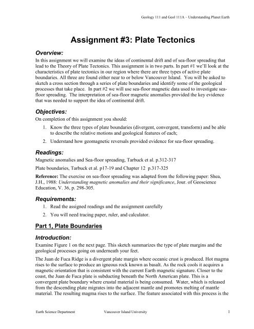
Assignment #3: Plate Tectonics - web.mala.bc.ca - Vancouver Island ...

Geology 111 and Geol 111A – Understanding Planet Earth
Assignment #3: Plate Tectonics
Overview:
In this assignment we will examine the ideas of continental drift and of sea-floor spreading that
lead to the Theory of Plate Tectonics. This assignment is in two parts. In part #1 we’ll look at the
characteristics of plate tectonics in our region where there are three types of active plate
boundaries. All three are found either near to or below Vancouver Island. You will be asked to
sketch a cross section through a series of plate boundaries and identify some of the geological
processes that take place. In part #2 we will use sea-floor magnetic data used to investigate seafloor
spreading. The interpretation of sea-floor magnetic anomalies provided the key evidence
that was needed to support the idea of continental drift.
Objectives:
On completion of this assignment you should:
1. Know the three types of plate boundaries (divergent, convergent, transform) and be able
to describe the relative motions and geological features of each;
2. Understand how geomagnetic reversals provided evidence for sea-floor spreading.
Readings:
Magnetic anomalies and Sea-floor spreading, Tarbuck et al. p.312-317
Plate boundaries, Tarbuck et al. p17-19 and Chapter 12 p.317-325
Reference: The exercise on sea-floor spreading was adapted from the following paper: Shea,
J.H., 1988: Understanding magnetic anomalies and their significance, Jour. of Geoscience
Education, V. 36, p. 298-305.
Requirements:
1. Read the assigned readings and the assignment carefully
2. You will need tracing paper, ruler, and calculator.
Part 1, Plate Boundaries
Introduction:
Examine Figure 1 on the next page. This sketch summarizes the type of plate margins and the
geological processes going on underneath your feet.
The Juan de Fuca Ridge is a divergent plate margin where oceanic crust is produced. Hot magma
rises to the surface to produce an igneous rock known as basalt. As the rock cools it acquires a
magnetic orientation that is consistent with the current Earth magnetic signature. Closer to the
coast, the Juan de Fuca plate is subducting beneath the North American plate. This is a
convergent plate boundary where crustal material is being consumed. Water, which is released
from the descending plate migrates into the adjacent mantle and promotes melting of mantle
material. The resulting magma rises to the surface. The feature associated with this process is the
Earth Science Department Vancouver Island University 1

Geology 111 and Geol 111A – Understanding Planet Earth
linear chains of volcanoes called the Cascadia volcanic belt. This belt stretches from Mendicino,
California to Bella Coola, BC, and includes volcanoes such as Mt. Shasta, Mt. St. Helens, Mt.
Rainier, Mt. Baker and Mt. Garibaldi. South of Mendicino and north of Bella Coola the oceanic
crust of the Pacific plate is not subducting, instead it is moving laterally relative to the North
American plate along the San Andreas and Queen Charlotte transform faults respecitively.
Transform
Fault
Mid
Ocean
Ridge:
Juan de
Fuca
Ridge
Transform
Fault
A
Triple
Junction
● Nanaimo
Figure 1. Showing local plate boundaries and their relative motions from Geological Survey of Canada
Pacific Geoscience Centre, 1999. Earthquakes and Plate Tectonics in Western Canada.
See < http://earthquakescanada.nrcan.gc.ca/index-eng.php > for more information.
Earth Science Department Vancouver Island University 2
A′
Subduction
Zone

Assignment 3: Part 1
Geology 111 and Geol 111A – Understanding Planet Earth
Name: ________________________
GEOL/Section: _______________________
Procedure:
Figure 1 shows a plan view of the geological processes occurring beneath Vancouver Island.
Your assignment is to sketch and label a cross section of the plates and illustrate how they are
moving relative to each other. (A cross-section is a view as if slicing through the earth). The
location of the section you are asked to sketch is marked by the line A-A' on Figure 1. Draw the
cross-section as viewing to the north.
The figures in Tarbuck et al. should help you to visualize what is occurring at plate tectonic
boundaries. There also is a poster on the wall in the lab (Geoscape Nanaimo) that also shows a
cut away view of the area of your assignment.
Start by drawing a line that depicts the approximate changes in elevation earth’s surface going
from the deep ocean floor at A to the Coast Mountains at A’. Then draw the location of the
tectonic plates below, with particular attention on the subduction zone and mid-ocean ridge.
Make sure you show the relative motions of the plates, the locations of any volcanic activity, the
source of magma, and indicate where you think earthquakes might occur.
A A’
Earth Science Department Vancouver Island University 3

Part 2, Sea-floor Spreading:
Introduction:
Geology 111 and Geol 111A – Understanding Planet Earth
Understanding the patterns of sea-floor magnetism:
A magnetometer is an instrument that is used to measure very small spatial variations in the
intensity of the earth’s magnetic field. Magnetometers can be moved around on land (usually by a
person on foot), in the air (towed beneath an aircraft) or at sea (towed behind a ship). Studies of
magnetic variations are useful in geological mapping and exploration for minerals because they
provide general information about variations in rock types (e.g. granite versus basalt), and about
the presence of rocks that have significantly more magnetic minerals than other rocks (e.g. iron
ores with magnetite).
During WWII, naval ships accompanying supply convoys crossing the Atlantic Ocean towed
sensitive magnetometers behind. These magnetometers were looking for submarines (a large
metal body capable of deflecting the Earth’s magnetic field locally). The operators of the
magnetometers found strange patterns of magnetic field reversals as they traversed the Atlantic.
In the mid-1950s the U.S. Office of Naval Research undertook a systematic oceanographic
survey of an area off the west coast. After much persuasion, they agreed to a request from the
Scripps Institute of Oceanography to tow a magnetometer behind the ship. The results of this
survey, which, for the first time, included many precisely located parallel survey lines, are shown
on Figure 2 below - a confusing, but systematic pattern of contrasting strips of positive
magnetism (black areas) and negative magnetism (white areas).
In the following years similar surveys were done in other areas - with similar results. However,
the origin of the patterns remained a mystery until 1963 when a solution was proposed by a
Cambridge graduate student (Fred Vine) and his thesis advisor (Drummond Matthews), and
(independently) by a Geological Survey of Canada Geologist (Lawrence Morely).
Vine, Matthews and Morely (VMM) suggested that the patterns could be related to the creation
of new oceanic crust at a spreading centre, and to the periodic reversals of the earth's magnetic
field. The idea is that as new basaltic crust is created its minerals (particularly magnetite) become
magnetized in alignment with the existing magnetic field of the earth. Rock formed during a
period of normal magnetism will give a positive magnetic anomaly because the rock has the same
polarity as the earth’s existing magnetic field, while rock formed during a period of reverse
magnetism will give a negative magnetic anomaly. The stripes on the ocean floor, it was
suggested, represent different ages of oceanic basaltic rock, which have been pushed away to
either side of a spreading centre and replaced by younger basaltic rock.
To begin with the VMM hypothesis was largely ignored, firstly because in the early 1960's the
idea of sea-floor spreading itself was not well accepted, secondly because the chronology of
magnetic-field reversals was not well known, and thirdly because there was not enough sea-floor
magnetic data to test the idea. Much more data became available within a few years, and once
others had a chance to verify the phenomenon for them selves the hypothesis became widely
accepted, and in fact played a crucial role in the general acceptance of continental drift and plate
tectonics a few years later.
Earth Science Department Vancouver Island University 4

Geology 111 and Geol 111A – Understanding Planet Earth
Figure 2 Systematic patterns of magnetic anomalies of the west coast of North America from Marshak, S.
2001: Earth, Portrait of a Planet.
Figure 3 Location of the Pacific Antarctic Ridge and profiles at 51.6S & 47.7S
Earth Science Department Vancouver Island University 5

Geology 111 and Geol 111A – Understanding Planet Earth
A confirmation of the Vine-Matthews-Morley hypothesis was made in 1966, when W. Pitman
analyzed several profiles of sea-floor magnetization across the Pacific-Antarctic Ridge (Figure
3), and found that one of the profiles, the Eltanin-19 profile, Figure 4, showed remarkable
symmetry, exactly as implied by the hypothesis.
In this exercise you will make a number of predictions based on the VMM hypothesis, and then
use some magnetic data to test them. Some useful predictions are as follows (although you might
be able to think of others):
since the spreading at a ridge is symmetrical on either side of the ridge axis, the pattern of
positive and negative magnetism should also be symmetrical,
magnetic profiles at various points along a ridge, and at different ridges around the world,
should be generally comparable,
the positive and negative magnetic features should correlate with the known chronology
of magnetic-field reversals, and
the corresponding rates of spreading (as determined from the magnetic chronology)
should be consistent with typical oceanic-ridge spreading rates (i.e. a few cm/year)
Figure 4 Sea-floor magnetic anomalies from the Eltanin-19 traverse.
Earth Science Department Vancouver Island University 6

Geology 111 and Geol 111A – Understanding Planet Earth
Assignment 3: Part 2 Name: ______________________________
GEOL/Section: ______________________
1) Symmetry across the ridge
Profiles of the magnetic patterns on the east and west sides of the Pacific-Antarctic ridge at 51.6º
S are shown on Figure 5. Compare the profiles - peak for peak and valley for valley. A good
way to do this is to trace the profile onto a separate sheet of paper and place it upside-down on
the other profile (axis to axis), and then hold the sheets up to the light. It is best to choose the
51.6 East profile to trace.
Figure 5. Magnetic profile at 51.6S on the west and east sides of the Pacific-Antarctic Ridge.
Earth Science Department Vancouver Island University 7

Geology 111 and Geol 111A – Understanding Planet Earth
Compare the profile you traced to the profile from the other side. (Note: make sure you hand in
your traced profile)
Q1. Do you think that the patterns are generally similar on opposite sides of the ridge, that is, do
they show a reasonable degree of biaxial symmetry? What might this biaxial symmetry mean?
2) Correlation along the ridge
A magnetic profile is available for the same ridge at 47.7º S (approx. 450 km north of the other
profile) and is shown on Figure 6 (east side only). A first glance this looks somewhat similar to
that of the east side profile at 51.6 S in Figure 5. However, in order to compare these profiles
more carefully, use the six well-defined positive peaks (normal polarity) that are identified and
labelled as: a, b, c, d, e & f on the 47.7º S profile (Figure 6), and identify the matching positive
peaks on the 51.6S (east side) profile in Figure 5.
For each of these peaks measure the distance in kilometres from the ridge axis (at 0) to the centre
of the peak using the scale given, and record the information in Columns 1 & 2 of Table 1. Then
calculate the ratio of the 47.7S profile distance to the 51.6S profile distance, and write that in
Column 3.
Figure 6 Magnetic profile at 47.7 S (east side) of the Pacific-Antarctic ridge.
Earth Science Department Vancouver Island University 8

Geology 111 and Geol 111A – Understanding Planet Earth
Q2: What does the ratio information tell you about the probable rates of spreading at these two
points on the ridge?
Peak
a
b
c
d
e
f
Column 1 Column 2 Column 3 Column 4 Column 5 Column 6 Column 7 Column 8
Distance
to peak
on east
side 51.6º
S (km)
Distance
to peak
on east
side 47.7º
S (km)
Distance
Ratio
Dist@
47.7S to
dist@
51.6S
Date of
magnetic
event
(Million
years, Ma)
Spreading
rate
(km/Ma) on
east side
51.6º S
Spreading
rate (km/Ma)
on east side
47.7º S
Average Spreading Rates – cm/year
Spreading
rate
(cm/year)
on east side
51.6º S
Table 1- Analysis of Data from east side of the Pacific Antarctic Ridge at Profiles 51.6S and 47.7S
Spreading
rate
(cm/year)
on east side
47.7º S
3) Correlation with the magnetic time-scale
The magnetic reversal time scale for the past 4.5 Ma is primarily derived from careful work
carried out on rocks of the continental crust, and is shown on Figure 7. Try to correlate some of
the peaks that you selected on Figures 5 or 6 with the various events described on this time scale,
and record the approximate dates of these events in Column 4 of the table above.
This is a difficult part of the assignment as it requires some level of ‘subjectivity’. Try and match
the widths of the peaks (which are in the normal magnetic fields) in one of the profiles (Figures 5
or 6) with the widths of the normal magnetic periods (black) found in Figure 7. Choose the
midpoint of the period of normal magnetism, which should correlate with the tip of the peak.
Earth Science Department Vancouver Island University 9

Geology 111 and Geol 111A – Understanding Planet Earth
Figure 7 Magnetic reversal events versus geological time, based on volcanic rocks on continental crust
Q3: From your matching exercise how well do the peaks of the magnetic profiles from the
Pacific-Antarctic ridge correlate with the chronology of magnetic field reversals found on
continental crust? What does this tell you?
4) Spreading Rate Calculations
Now that you have an estimate of distance (km) and time (Ma) it is possible to determine the
speed of ocean plate growth or more correctly the ‘spreading rate’ of oceanic crust. For each peak
and each profile do this by dividing the distances (km) by the date of the magnetic event (Ma)
and fill in Columns 5 and 6.
However, we typically think of plate movement in terms of cm/year which is easier to visualize
rather than km/years. In order to do this you will have to convert you results in Columns 5 and 6
from km/Ma to cm/year. Once you have figured out how to do this fill in Columns 7 and 8.
In order to get an average for the spreading rates at the two locations add the spreading rates and
divide by the number of peaks or sample points. Report your final averages in the table.
Q4 Are these reasonable rates for a spreading ridge? How do they compare to rates reported in
your textbook? Do your findings satisfy Vine Matthews and Morely (VMM)’s hypothesis for
sea-floor spreading? What does this evidence support in terms of the plate tectonic theory?
Earth Science Department Vancouver Island University 10