- Page 2 and 3:
A Handbook of Statistical Analyses
- Page 4 and 5:
Preface SPSS, standing for Statisti
- Page 6 and 7:
Distributors The distributor for SP
- Page 8 and 9:
3 Simple Inference for Categorical
- Page 10 and 11:
10 Survival Analysis: Sexual Milest
- Page 12 and 13:
1. SPSS Base (Manual: SPSS Base 11.
- Page 14 and 15:
Display 1.1 Initial SPSS for Window
- Page 16 and 17:
Display 1.3 Variable View window of
- Page 18 and 19:
three-periods symbol and filling in
- Page 20 and 21:
Display 1.6 Opening an existing SPS
- Page 22 and 23:
Display 1.8 Typical dialogue box. s
- Page 24 and 25:
Transpose… opens a dialogue for s
- Page 26 and 27:
Display 1.11 Selecting subsets of c
- Page 28 and 29:
A large number of functions are sup
- Page 30 and 31:
Display 1.15 Graph procedures demon
- Page 32 and 33:
More than one Output Viewer can be
- Page 34 and 35:
The Chart Editor facilities are des
- Page 36 and 37:
Display 1.19 Syntax Editor showing
- Page 38 and 39:
Table 2.1 Lifespans of Rats (in Day
- Page 40 and 41:
The test-statistic is where - y 1 a
- Page 42 and 43:
For small samples, p-values for the
- Page 44 and 45:
Display 2.1 Data View spreadsheet f
- Page 46 and 47:
lifespan in days diet Restricted di
- Page 48 and 49:
Lifespan in days 1600 1400 1200 100
- Page 50 and 51:
Display 2.6 Settings for controllin
- Page 52 and 53:
Display 2.8 Generating an independe
- Page 54 and 55:
Display 2.10 Generating a Mann-Whit
- Page 56 and 57:
Display 2.13 Generating descriptive
- Page 58 and 59:
simply because ages were measured o
- Page 60 and 61:
Display 2.18 Generating a Wilcoxon
- Page 62 and 63:
Husbands' ages (years) 80 70 60 50
- Page 64 and 65:
Display 2.24 Generating correlation
- Page 66 and 67:
Display 2.26 Fitting a simple linea
- Page 68 and 69:
Table 2.4 Motor Vehicle Theft in th
- Page 70 and 71:
2.4.5 More on Husbands and Wives: E
- Page 72 and 73:
Table 3.1 Belief in the Afterlife B
- Page 74 and 75:
make up the table. Most commonly, a
- Page 76 and 77:
This is known as a hypergeometric d
- Page 78 and 79:
(2) Odds ratio The odds of Variabl
- Page 80 and 81:
Display 3.2 Cross-classifying two c
- Page 82 and 83:
Odds Ratio for diet (Restricted die
- Page 84 and 85:
Display 3.7 Data View spreadsheet f
- Page 86 and 87:
Display 3.10 Generating a chi-squar
- Page 88 and 89:
20 10 Observed number 30 0 Psychoti
- Page 90 and 91:
Chi-Square Tests Value McNemar Test
- Page 92 and 93:
Pearson Chi-Square Likelihood Ratio
- Page 94 and 95:
Race of defendant found guilty of m
- Page 96 and 97:
Estimate ln(Estimate) Std. Error of
- Page 98 and 99:
treatment are independent. Estimate
- Page 100 and 101:
Table 4.1 Cleaning Cars Sex (1 = ma
- Page 102 and 103:
Table 4.2 (continued) Minimum Tempe
- Page 104 and 105:
A measure of the fit of the model i
- Page 106 and 107:
Display 4.2 Generating the partial
- Page 108 and 109:
We specify the dependent variable a
- Page 110 and 111:
for the coefficient is given by [0.
- Page 112 and 113:
Display 4.7 Setting inclusion and e
- Page 114 and 115:
Model 1 2 Model 1 2 Variables Enter
- Page 116 and 117:
proportion of variance of the varia
- Page 118 and 119:
The final graph shown in Display 4.
- Page 120 and 121:
Display 4.12 Generating a scatterpl
- Page 122 and 123:
Model 1 Model 1 Model Summary .973a
- Page 124 and 125:
Display 4.15 Blocking explanatory v
- Page 126 and 127:
1. Residual plot: This is a scatter
- Page 128 and 129:
8 6 4 Frequency 10 2 0 2.25 1.75 1.
- Page 130 and 131:
a) Latitude January minimum tempera
- Page 132 and 133:
Display 4.22 Extending a spreadshee
- Page 134 and 135:
Table 4.4 Sulfur Dioxide and Indica
- Page 136 and 137:
Table 4.5 Body Fat Content and Age
- Page 138 and 139:
Table 5.1 Fecundity of Fruit Flies
- Page 140 and 141:
Table 5.3 Female Social Skills Anxi
- Page 142 and 143:
There are some advantages (and, unf
- Page 144 and 145:
Display 5.1 SPSS spreadsheet contai
- Page 146 and 147:
Display 5.3 Defining a one-way desi
- Page 148 and 149:
Dependent Variable: FECUNDIT Tukey
- Page 150 and 151:
Click Simple in the resulting Error
- Page 152 and 153:
finger taps per minute Between Grou
- Page 154 and 155:
Display 5.13 Defining a one-way des
- Page 156 and 157:
5.0 4.0 Mean score 6.0 3.0 2.0 B. r
- Page 158 and 159:
the data to assess whether the assu
- Page 160 and 161:
Chapter 6 Analysis of Variance II:
- Page 162 and 163:
Table 6.2 Data from Slimming Clinic
- Page 164 and 165:
When the cells of the design have d
- Page 166 and 167:
Dependent Variable: reaction time p
- Page 168 and 169:
Display 6.5 Requesting a line chart
- Page 170 and 171:
Display 6.8 Confidence intervals fo
- Page 172 and 173:
MANUAL Total manual no manual MANUA
- Page 174 and 175:
In a balanced design, the type I, I
- Page 176 and 177:
6.4 Exercises 6.4.1 Headache Treatm
- Page 178 and 179:
ANCOVA assumes that there is no int
- Page 180 and 181:
Table 7.1 Field Independence and a
- Page 182 and 183:
or error term. The u i are assumed
- Page 184 and 185:
To convey this design to SPSS, the
- Page 186 and 187:
LN_FN LN_FC LN_FI LN_CN LN_CC LN_CI
- Page 188 and 189:
Within-Subjects Factors Measure: ME
- Page 190 and 191:
Measure: MEASURE_1 Within Subjects
- Page 192 and 193:
e used, or for a conservative appro
- Page 194 and 195:
Table 7.2 Visual Acuity and Lens St
- Page 196 and 197:
Chapter 8 Analysis of Repeated Meas
- Page 198 and 199:
Table 8.1 A Subset of the Data from
- Page 200 and 201:
Table 8.1 (continued) A Subset of t
- Page 202 and 203:
Box 8.1 Random Effects Models Supp
- Page 204 and 205:
0 10 20 30 Response Average group 1
- Page 206 and 207:
95% CI for mean score 30 20 10 0 N
- Page 208 and 209:
a) TAU group Baseline depression sc
- Page 210 and 211:
Display 8.6 Part of Data View sprea
- Page 212 and 213:
Display 8.7 Defining the variables
- Page 214 and 215:
variables; and the variance paramet
- Page 216 and 217: Fixed Effects Random Effects Residu
- Page 218 and 219: different post-treatment time point
- Page 220 and 221: Iteration 0 1 2 3 4 5 6 7 8 Update
- Page 222 and 223: a) Estimates of error term (residua
- Page 224 and 225: Table 8.3 Depression Ratings for Su
- Page 226 and 227: Constant error variance across repe
- Page 228 and 229: Display 9.1 Characteristics of 21 T
- Page 230 and 231: Competing models in a logistic regr
- Page 232 and 233: Survived? Total Survived? Total no
- Page 234 and 235: Display 9.4 Defining a five-way tab
- Page 236 and 237: Display 9.6 Defining a logistic reg
- Page 238 and 239: Step 1 a Step 1 PCLASS PCLASS(1) PC
- Page 240 and 241: Table 9.1 Unadjusted Effects of Cat
- Page 242 and 243: of all explanatory variables simult
- Page 244 and 245: Step 1 a Table 9.2 LR Test Results
- Page 246 and 247: log-odds of survival log-odds of su
- Page 248 and 249: 9.4 Exercises 9.4.1 More on the Tit
- Page 250 and 251: Chapter 10 Survival Analysis: Sexua
- Page 252 and 253: Table 10.1 (continued) Times to Fir
- Page 254 and 255: Table 10.2 Times to Completion of t
- Page 256 and 257: To compare the survivor functions b
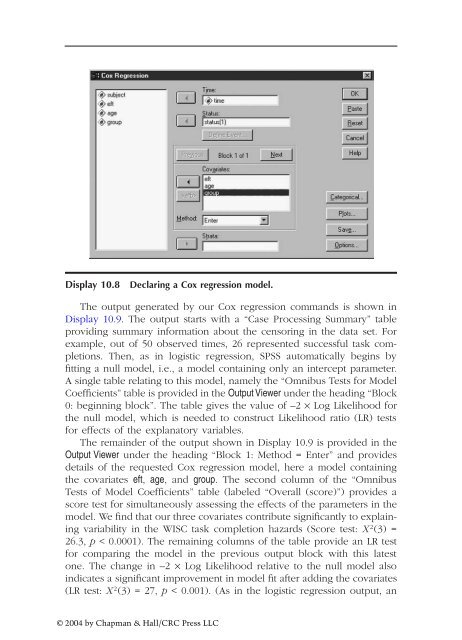
- Page 258 and 259: 10.3 Analysis Using SPSS 10.3.1 Sex
- Page 260 and 261: Display 10.2 Generating Kaplan-Meie
- Page 262 and 263: Survival Analysis for AGESEX Age of
- Page 264 and 265: Display 10.6 Requesting tests for c
- Page 268 and 269: Cases available in analysis Cases d
- Page 270 and 271: Display 10.10 Plotting the predicte
- Page 272 and 273: Display 10.12 Saving results from a
- Page 274 and 275: The smooth lines in the respective
- Page 276 and 277: EFT AGE Display 10.15 Selected outp
- Page 278 and 279: Table 10.3 Heroin Addicts Data Subj
- Page 280 and 281: Table 10.3 (continued) Heroin Addic
- Page 282 and 283: Table 11.1 Crime Rates in the U.S.
- Page 284 and 285: Table 11.2 AIDS Patient’s Evaluat
- Page 286 and 287: that need to be considered. If the
- Page 288 and 289: the analysis is based on the correl
- Page 290 and 291: We assume that the residual terms a
- Page 292 and 293: Correlation Murder Rape Robbery Agg
- Page 294 and 295: Murder Rape Robbery Aggravated assa
- Page 296 and 297: Display 11.6 Saving factor scores.
- Page 298 and 299: Display 11.8 Requesting descriptive
- Page 300 and 301: a) One-factor model Goodness-of-fit
- Page 302 and 303: Raw Rescaled Factor 1 2 3 4 5 6 7 8
- Page 304 and 305: friendly manner doubts about abilit
- Page 306 and 307: Display 11.16 Reproduced covariance
- Page 308 and 309: 11.4.2 More on AIDS Patients’Eval
- Page 310 and 311: Table 12.1 Tibetan Skulls Data Skul
- Page 312 and 313: Euclidean distances are the startin
- Page 314 and 315: Fisher showed that the coefficients
- Page 316 and 317:
Display 12.2 Declaring a discrimina
- Page 318 and 319:
Box's M F Display 12.4 (continued)
- Page 320 and 321:
Display 12.6 (continued) Functions
- Page 322 and 323:
Original Cross-validated a place wh
- Page 324 and 325:
Display 12.10 Requesting a dendrogr
- Page 326 and 327:
* * * * * * H I E R A R C H I C A L
- Page 328 and 329:
Display 12.14 Declaring a k-means c
- Page 330 and 331:
12.4 Exercises Cluster Number of Ca
- Page 332 and 333:
Table 12.2 (continued) SIDS Data Gr
- Page 334 and 335:
References Agresti, A. (1996) Intro
- Page 336 and 337:
Greenhouse, S. W. and Geisser, S. (
- Page 338:
Stevens, J. (1992) Applied Multivar