Feature-based Extrinsic Calibration of Camera and 3D Laser Range ...

Semester-Thesis
Feature-based Extrinsic
Calibration of Camera and
3D Laser Range Finder
Spring Term 2010
Autonomous Systems Lab
Prof. Roland Siegwart
Supervised by: Author:
Jérôme Maye Stefan Dahinden
Ralf Kaestner

Contents
Abstract iii
Preface v
1 Introduction 1
2 Related Work 3
2.1 Extrinsic Calibration . . . . . . . . . . . . . . . . . . . . . . . . . . . 3
2.1.1 Point Cloud Registration . . . . . . . . . . . . . . . . . . . . 3
2.2 Feature Extraction . . . . . . . . . . . . . . . . . . . . . . . . . . . . 4
2.2.1 Features from Camera . . . . . . . . . . . . . . . . . . . . . . 4
2.2.2 Features from 3D Laser Range Finder . . . . . . . . . . . . . 4
3 Specifications 7
3.1 Camera . . . . . . . . . . . . . . . . . . . . . . . . . . . . . . . . . . 7
3.2 3D Laser Range Finder . . . . . . . . . . . . . . . . . . . . . . . . . 7
3.3 Data Acquisition . . . . . . . . . . . . . . . . . . . . . . . . . . . . . 8
3.3.1 Scene . . . . . . . . . . . . . . . . . . . . . . . . . . . . . . . 8
4 Approach 9
4.1 Possible Features . . . . . . . . . . . . . . . . . . . . . . . . . . . . . 9
4.2 Registration Algorithm . . . . . . . . . . . . . . . . . . . . . . . . . . 10
4.3 Method for Extrinsic Parameter Estimation . . . . . . . . . . . . . . 11
5 Implementation 13
5.1 Framework . . . . . . . . . . . . . . . . . . . . . . . . . . . . . . . . 13
5.2 Interface . . . . . . . . . . . . . . . . . . . . . . . . . . . . . . . . . . 13
5.3 Feature Extraction . . . . . . . . . . . . . . . . . . . . . . . . . . . . 14
5.3.1 Canny Edge Detector . . . . . . . . . . . . . . . . . . . . . . 14
5.3.2 Harris Corner Detector . . . . . . . . . . . . . . . . . . . . . 15
5.3.3 SURF Detector . . . . . . . . . . . . . . . . . . . . . . . . . . 16
5.3.4 3D SURF Implementation . . . . . . . . . . . . . . . . . . . . 17
5.3.5 3D Hough Transform . . . . . . . . . . . . . . . . . . . . . . . 17
5.3.6 Depth Image . . . . . . . . . . . . . . . . . . . . . . . . . . . 18
5.4 Image Registration . . . . . . . . . . . . . . . . . . . . . . . . . . . . 19
5.5 Extrinsic Parameter Estimation . . . . . . . . . . . . . . . . . . . . . 21
6 Results 23
6.1 Features . . . . . . . . . . . . . . . . . . . . . . . . . . . . . . . . . . 23
6.2 ICP . . . . . . . . . . . . . . . . . . . . . . . . . . . . . . . . . . . . 24
6.3 Extrinsic Parameter Estimation . . . . . . . . . . . . . . . . . . . . . 24
i

7 Discussion 27
7.1 Feature Combinations . . . . . . . . . . . . . . . . . . . . . . . . . . 27
7.2 Registration Algorithm . . . . . . . . . . . . . . . . . . . . . . . . . . 27
7.3 Approximation of Extrinsic Parameters . . . . . . . . . . . . . . . . 28
8 Future Work 29
8.1 Improvements to Feature Extraction . . . . . . . . . . . . . . . . . . 29
8.1.1 Bearing Angle Images . . . . . . . . . . . . . . . . . . . . . . 29
8.1.2 Automatic Thresholding . . . . . . . . . . . . . . . . . . . . . 30
8.2 Registration Process . . . . . . . . . . . . . . . . . . . . . . . . . . . 30
8.2.1 Outlier Rejection . . . . . . . . . . . . . . . . . . . . . . . . . 30
9 Conclusion 31
Bibliography 33
ii

Abstract
This thesis documents the implementation and evaluation of an automated method
for the estimation of the extrinsic calibration between a 3D laser range finder and
a camera. In contrast to common calibration systems, this method is based on
features. No calibration pattern has to be introduced.
In a first step, several feature extraction methods are implemented. The features
are then evaluated for a later registration method. The selected features are used to
register the two data sets. ICP is applied for this process. The registrated features
are then plugged into a least squares method to estimate the extrinsic calibration
parameters.
It is shown in this thesis that it is possible to create a feature-based method for
extrinsic calibration. The features that were selected due to a promising visual
match are the Canny edge detector for the camera data and the Harris corner
detector for the depth image coming from the 3D laser range finder.
iii

Preface
During the last fourteen weeks I implemented and evaluated an interface allowing
to estimate the extrinsic calibration parameters between a camera and a 3D laser
range finder. The extrinsic calibration of a sensor setup is a very basic problem that
often appears in modern robotics. It is common to solve it by manually selecting
some corresponding features or with the help of a calibration pattern. Therefore
the idea of creating a feature-based fully automated method fascinated me.
I enjoyed working at the Institute for Robotics and Intelligent Systems in the Autonomous
Systems Lab (ASL) which is led by Prof. Roland Siegwart. It was
interesting to get an insight in the current research topics of the lab.
I thank my tutors, Jérôme Maye and Ralf Kaestner for their valuable help, rich
feedback and for spending many hours advising me in our weekly meetings. I thank
my supervisor Prof. Roland Siegwart who made this thesis possible and supported
me by granting me a workplace. I also would like to thank Mario Deuss who helped
me with a fast implementation of the depth image.
Zurich, July 25, 2010
Stefan Dahinden
v

Chapter 1
Introduction
In most robotic systems there is a multi modal sensor setup present to perceive
the environment. The data from a set of different sensor types is merged into a
believe state about the position of the robot, the structure and characteristics of
the environment or the dynamics of the surrounding objects. There is also the
possibility to reconstruct certain regions of the surrounding three dimensionally for
a later manual inspection.
To be able to merge the data of various types of sensors, different approaches are
used. Stochastic approaches can create a probability distribution of the believe
state of the current position of the robot. There are also several techniques that
are based on machine learning algorithms to find certain objects in the sensor data.
Bio-inspired algorithms suggest actions to accomplish predefined longterm tasks.
And analytical methods may help to find fast solutions and first guesses that can
then be refined by other algorithms.
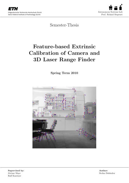
Figure 1.1: A possible scene in modern robotics.
All these methods rely on a good calibration of the multi modal sensor setup.
In most of the cases, the intrinsic calibration of each sensor is known or can be
calculated easily. On the other hand it is not so easy to measure an exact extrinsic
calibration. As most of the sensor types used in todays robots are measuring in a
radial manner, especially the orientation of a sensor is extremely important. Even
a small angular deviation can lead to large errors in the interpretation of the sensor
data. Therefore a data based extrinsic calibration method is vital.
There are several approaches of data based extrinsic calibration known to the au-
1

Chapter 1. Introduction 2
thor. All of them include one or both actions from the following list.
• Artificially altering the environment: This can either be done by the
introduction of a calibration pattern as shown in Figure 1.2 or by specific
illumination of the environment (light grids or dots).
• Manual selection of corresponding points: The user has to manually
select points in the different sensor data spaces. These point pairs should
coincide spatially.
Figure 1.2: A scene with a calibration pattern (checkerboard).
The idea of this thesis is to do a feature-based approach of selecting spatially coincident
point pairs. This will erase the necessity of either artificially altering the
environment or manually selecting point pairs.

Chapter 2
Related Work
2.1 Extrinsic Calibration
Different calibration techniques have been proposed over the last years [31, 28, 27,
13, 7]. Most of the techniques have the goal to texture 3D models with camera
images of the same scene [20, 7]. These scenes can then be used for localization
estimation, map building, visual inspection or even digital archiving of historic
objects or buildings.
There exist several Matlab Toolboxes for an efficient and robust calibration of camera
and 3D laser range finder [28, 31]. Some of them need interaction with the user
by locating corresponding feature pairs [28]. Often a checkerboard is used as a calibration
pattern which can be automatically detected [32, 27, 31]. Another technique
of introducing a artificial calibration pattern is the use of light grids [33, 18].
All these approaches are based on selecting spatially corresponding points of the
datasets of both camera and 3D laser range finder. From this point correspondences
the extrinsic parameters can then be estimated by minimizing the distance between
the point pairs.
2.1.1 Point Cloud Registration
As this thesis points towards a feature-based approach which replaces the manual
selection by a user, a registration algorithm is needed to find correspondences
between the feature sets.
Many registration methods have been developed for pose estimation [4, 34]. Some
of them work with features and feature descriptors. Furthermore the computational
complexity is rather high. Either a large feature descriptor is used which has to
be compared over the features or decompositions are calculated on large matrices.
Additionally all of these feature-based approaches assume data from the same type
of sensor. The most common sensor type in these cases is the camera. Our thesis
works with two different types of sensors - camera and 3D laser range finder.
Therefore, these approaches are not well suited for the problem of this thesis.
The most popular registration algorithm suitable for point clouds is the iterated
closest point method (ICP). It is a very simple approach introduced by several researchers
at nearly the same time [33, 3, 8, 6]. The principle idea is to start at
an initial guess of the position and orientation. By iteratively adapting the transformation
to minimize the distance between the current neighbors, ICP converges
to the optimum if the initial guess was good enough. Several improvements have
been proposed to the basic ICP. A fast implementation using search index trees
was developed [29]. To further improve the stability of the algorithm, the distance
function was extended by taking surface normals into account [11].
3

Chapter 2. Related Work 4
2.2 Feature Extraction
A feature-based registration method needs robust features in both datasets. In
the following subsections all feature detectors are presented that were used and
evaluated in this thesis.
2.2.1 Features from Camera
Many feature extraction methods exist for camera images [26]. In 1986 Canny
proposed a gradient based edge detector [5]. He takes the gradient magnitude and
performs a non maximum suppression in direction of the gradient. This results
in very robust edge features. Canny also derived a computational theory of edge
detection to explain his method. Although the Canny operator was proposed very
early it is still used very often due to his simple approach and robust features.
Two years later, Harris introduced a combined edge and corner detector which is
based on directional derivatives [15]. A matrix is built up for every pixel using
a sum of directional derivatives in a sliding window. With the eigenvalue of this
matrix one can decide whether the pixel is a corner, an edge or a flat region.
Besides edges and corners, blob like structures can also be detected robustly in
camera images. Basically two simple approaches exist that can detect blobs. Both
rely on filters that are convolved with the image and result in large absolute values
in a blob and low values otherwise.
• Laplacian of Gaussian (LoG): By taking the Laplacian of the convolution
of the image with a Gaussian kernel, blobs show a strong answer. To render
this approach scale invariant, several convolutions with differently scaled
Gaussian kernels are applied. Local extrema in both scale and spacial space
are then extracted. There is also the possibility to approximate the Laplacian
of Gaussian by a difference of Gaussian convolutions (DoG) with the image.
• Determinant of the Hessian (DoH): Another approach is to compute
the Hessian matrix and then take the scale-normalized determinant to detect
blobs [21, 22]. The SIFT feature descriptor exploits this method to detect its
features [23, 24]. Approximating the Hessian determinant with Haar wavelets
results in the basic interest point operator of the SURF descriptor [2].
2.2.2 Features from 3D Laser Range Finder
While many stable feature detectors exist for camera images, few have been introduced
for point clouds of 3D laser range finder. One reason for this is the higher
dimensionality and therefore higher computational complexity of the methods. This
leads to a lower usability in practical applications. Another reason could be that
3D laser range finder are much slower in the gathering of a dataset.
The probably simplest approach is to perform a Hough transform which can be
used whenever the data is a point cloud. The Hough transform projects every
point of the point cloud into a parameter space [16, 1]. The parameters model a
certain shape. Often planes or lines are used. The best responses in the Hough
space can then be transformed back to the spacial space where they represent a
shape with defined parameters. Several improvements have been proposed such as a
probabilistic approach [19], a refinement of the line parametrization by using normal
parameters [10] or an adaptive variation which is an efficient way of implementing
the Hough transform [17]. The biggest argument for the Hough transform is its
universality. Although computational complexity can become a problem, the Hough
transform works on a huge range of data structures and can detect every shape that
is parameterizable with a small amount of parameters.

5 2.2. Feature Extraction
Another feature extractor for 3D point clouds is the ThrIFT operator [14]. ThrIFT
is a 3D adaptation of the SIFT descriptor. According to the author, the features
are robust but unfortunately not very distinctive.
Methods for estimating surface normals in 3D point clouds have also been proposed
[25]. With the help of the surface normals, the points can then be connected to
a mesh. The mesh can provide information about edges and corners in the point
cloud.
Higher dimension and the nature of the point cloud result in higher computational
complexity. Therefore in many cases a reduction of the dimensionality is applied.
Often this is done by working with a depth image [28]. Especially for data from a
3D laser range finder which consists of already sorted data points. Operating on
depth images has the huge advantage that any feature detector applicable on 2D
images can be used.

Chapter 2. Related Work 6

Chapter 3
Specifications
In this chapter, technical details about the sensors and the measured scenes are
presented. The sensor setup consists of a 3D laser range finder and a camera (see
Figure 3.1).
3.1 Camera
The camera used in the setup was a XCD SX910CR from Sony. It has a fixed focal
length of 4.3mm and takes pictures at a resolution of 1280x960 pixels. No flash was
used and the pictures were not post processed.
Figure 3.1: Left: Camera (Sony XCD SX910CR), Right: Laser range finder (Sick
LMS 200).
3.2 3D Laser Range Finder
A Sick LMS 200 laser range finder was used to gather the 3D data. It is mounted
on a servo motor so it can be tilted from -45 ◦ to 45 ◦ at an angular resolution of
7

Chapter 3. Specifications 8
1 ◦ . At every angular step around the pitch axis a scan around the current yaw axis
from -90 ◦ to 90 ◦ is performed with 1 ◦ steps at 75 Hz. The laser range finder can
measure distances up to ca. 80m at an accuracy of 35mm. It is directly connected
to a laptop and produces a single log file containing all measurements each with a
time step attached.
3.3 Data Acquisition
The data was taken simultaneously to prevent changes in illumination or the placement
of any objects in the scene. The sensor setup can be seen in Figure 3.1.
3.3.1 Scene
To gather the data, indoor scenes were chosen as well as an outdoor scene. A
picture of an indoor scene can be seen in Figure 3.2. The scene was illuminated by
Figure 3.2: One of the scenes.
the already installed lamps. Also the measurements were performed during daytime
and the windows were not covered. No additional light was introduced. The scene
was not artificially changed with a calibration pattern.

Chapter 4
Approach
The goal of this thesis is to assess the realization of a completely automated method
for extrinsic parameter estimation between a camera and a 3D laser range finder.
The method should rely on features extracted from measurements taken simultaneously
from both sensors in an indoor scene.
To achieve this task all of the following steps have to be implemented:
• Preprocessing: The data sets from both sensors are preprocessed in a first
step to prepare them for an efficient and robust feature extraction.
• Feature extraction: Features are then extracted from both datasets. It
is important to note that this features should be chosen in a way that they
can be registered in a later step. However, this does not mean that the same
feature extraction method has to be chosen for both data sets.
• Feature registration: The extracted features are then registrated to find
spatially matching features. For this task, not only the spatial information of
the features are available but also feature descriptors that can be directly created
from the data sets. This step therefore tries to solve the correspondence
problem. As a result, we get matching feature pairs over the two datasets.
• Estimation of extrinsic parameters: By using the matched feature pairs
the extrinsic calibration of camera and 3D laser range finder can then be
estimated in a last step. There are three rotational and three translational
degrees of freedom. Therefore this is a six degrees of freedom problem that
has to minimize a predefined error function based on the distance between the
matched features.
4.1 Possible Features
As already discussed in Chapter 2 the variety of feature detectors available for
camera images is large. It is a priori not clear what features to use. Therefore a
selection of promising feature detectors was formed. The same was done for possible
methods for data coming from a 3D laser range finder.
In the following all features evaluated in this thesis are listed.
• Camera Features
– Canny edge detector
– Harris corner detector
– SURF
9

Chapter 4. Approach 10
• Features for 3D point clouds
– Hough transform
– 3D SURF
– Features from depth image
∗ Canny edge detector
∗ Harris corner detector
∗ SURF
The features were chosen for different reasons. Firstly, the features have to be
stable in the scenes we used. Secondly, since features that are often used in related
work have been refined and adapted into different variations, they are more
promising to this thesis. This can be explained by the flexibility of the respective
approaches. They have proven to be stable and distinctive in various situations and
were compared against other feature detectors several times. Thirdly, the features
were chosen in a way that the detected interest points cover a wide range of different
objects.
For the camera three feature extractors were chosen. The Canny edge detector is
based on both the gradient magnitude as well as the gradient orientation of the
image [5]. The Harris corner detector is based on directional derivatives and works
with a matrix constructed of weighted sums of these derivatives in a sliding window
[15]. The newest feature detector in the list is the SURF detector introduced by
Bay in 2006 [2]. It is capable of detecting blob like structures in the image. By
looking at the determinant of an estimation of the Hessian matrix it is able to find
blobs at any scale in the image. Through the exploitation of integral image these
estimations can be calculated in constant time at any scale using box filters.
For the 3D point cloud there are two possibilities to extract features. Either by
working with the raw point cloud and therefore extracting 3D features. Or by
computing the depth image from the point cloud and applying common 2D feature
extraction methods. For the 3D case two feature extraction methods were used.
The Hough transform was used to extract arbitrary planes through the point cloud
that are supported by many points in the cloud [1]. From these planes, 3D edges
and corners can then be calculated. A 3D implementation of the SURF detector
was developped to extract blob like 3D structures like a teapot on a table or a lamp
hanging from the ceiling.
From the depth map the same features were chosen as for the camera image. The
reasons are the same as for the features for the camera image. Additionally, the use
of the same features might help the registration process.
The different feature extraction methods were then compared to each other in order
to find combinations of features from camera image and 3D point cloud that are well
suited for each other. This assessment was done with regard to a later registration
process.
4.2 Registration Algorithm
After the features are extracted they must be registrated. This means that spatially
corresponding features from both feature sets have to be matched with each other.
Several approaches have been proposed (see Chapter 2).
For this thesis a basic approach had to be chosen. This ensures the possibility of
introducing additional information as help for the registration. As a registration
algorithm for point clouds in both 2D and 3D, ICP has proven very powerful in
many ways.

11 4.3. Method for Extrinsic Parameter Estimation
Firstly, it is a very straightforward iterative process. In every iteration points from
both data sets are assigned to each other with a nearest neighborhood criteria.
Then a new transformation is approximated that minimizes the distance between
the assigned points. The new transformation is then applied to the original dataset.
This process is iterated until convergence.
Secondly, the introduction of a feature descriptor fits nicely into the definition of
the algorithm. By adding weights to each assigned point pair based on the distance
of their descriptors, the minimization process takes the gradient orientation into
account. However it is not possible to introduce a intensity based feature descriptor
because of the two sensor types. Although the images contain some similar information,
the way of representing this information is different. Therefore a intensity
based comparator like correlation in a sliding window is not feasible.
For all its advantages ICP has also a drawback. An initial transformation guess
is needed to start the iteration process. Therefore it is unavoidable to state some
assumptions when using ICP. With the help of the intrinsic calibration it is of
course possible to match both datasets together when the extrinsic calibration is
the identity. If the changes to location and orientation are small, the intrinsic
calibration is a good initial guess of the transformation. Therefore the assumption
is introduced that the changes in location and orientation are small. Then the
intrinsic calibration of the camera can be used as an initial guess.
4.3 Method for Extrinsic Parameter Estimation
After the registration process a set of matched features is available that are spatially
close to each other. From these point pairs the extrinsic parameters have to be
estimated in a last step. This is a basic least squares problem with six degrees of
freedom. It can be solved using many methods. The chosen approach creates a
matrix A containing the system of equations that states the initial problem. By
minimizing the norm of the product ||A · x||, x is retrieved. From x, the extrinsic
calibration matrix can easily be obtained. The exact methodology can be found in
Chapter 5.

Chapter 4. Approach 12

Chapter 5
Implementation
In this chapter the implementation of the extrinsic calibration process is explained
and encountered challenges are illustrated.
5.1 Framework
Since this thesis does not build upon a specific previous work the choice of the
language and environment was completely free. Matlab [30] was chosen due to
several reasons. Firstly, it is data oriented and has therefore a very natural and
clear way of working with data. Secondly, it is very easy to create output, both
visual and text. An image or graph can be plotted in one single command. Thirdly,
as long as it is used proper, the language is reasonably fast. Fourthly, Matlab has a
rich selection of official functions that are organized in toolboxes. The functions are
well documented and the support answers fast and appropriate. Last but not least,
Matlab is a platform independent environment which encouraged a large community
of users to create additional content by offering various functions that complement
the toolboxes.
5.2 Interface
As there is little interaction with the user the interface is kept simple. A screen shot
can be seen in Figure 5.1. There is written output in the command stream to show
which step is currently performed and how long the previous steps took. There are
also several figures. One of them can be seen in the screen shot showing the currently
matched features during the ICP iterations. There are other figures showing all the
extracted features, the final calibration as two coordinate frames translated and
rotated properly to each other. At termination of the script the rotational part of
the extrinsic calibration is stored in the three dimensional rotation matrix R, the
translational part in the vector C and the intrinsic calibration matrix in K. This
leads to
pcam = K · (R · plrf + C)
where pcam is a point in the camera image and plrf is a point in the point cloud of
the laser range finder. A pinhole model was chosen as approximation for the camera
used in this thesis.
13

Chapter 5. Implementation 14
Figure 5.1: The interface on Matlab R2008b.
5.3 Feature Extraction
Several feature detection methods had to be implemented during this thesis. An
exact description of the functionality and mathematical implementation of each of
them is given below.
5.3.1 Canny Edge Detector
As described in Chapter 2 the Canny edge detector is a gradient based edge detector
proposed by John Canny in 1986 [5]. The detector is divided into four stages.
Noise Reduction In the first stage present noise is suppressed. This prevents
noisy features due to the fact that the Canny edge detector is rather sensitive to
pixel noise present on most unprocessed images. The noise reduction is done by
convolving the original image with a Gaussian filter. Gaussian filters blur the image
to a certain extent, depending on the filter size and the σ that was chosen for the
filter.
Figure 5.2: Canny edge features.

15 5.3. Feature Extraction
Computation of Gradient As the gradient of a pixel is high if an edge is present,
the gradient magnitude and gradient orientation is calculated in a second step. The
first derivative in both horizontal and vertical direction Gx and Gy are approximated
using certain filters (Prewitt and Sobel are examples that can approximate the
derivatives). The gradient magnitude and gradient orientation
G =
Θ = arctan
G2 x + G2 y
Gy
can then be calculated. The gradient orientation is then rounded to one of the
four angles 0 ◦ (vertical, N), 45 ◦ (diagonal, NE), 90 ◦ (horizontal, E) and 135 ◦ (other
diagonal, SE).
Non-maximum Suppression After computing the gradient magnitude, a nonmaximum
suppression is performed on the gradient magnitude in direction of the
gradient orientation. For example, if a pixel has a gradient orientation of 0 ◦ , the
pixel is set to zero if the neighboring pixels in either north or south direction has
a larger gradient magnitude. The pixel is set to one otherwise. This results in a
binary image where edge candidates have the value one.
Edge Tracing by hysteresis thresholding In a last step noisy edges are suppressed.
This is done by two thresholds. Every pixel with a gradient magnitude
greater than the higher threshold is classified as belonging to an edge for sure.
From every edge point found with the high threshold, the edge can be traced in
both directions using the directional information derived earlier. Applying the lower
threshold allows to trace edges even through unclear regions as long as the gradient
magnitude stays above the threshold.
This process results in another binary image with clean edges that are connecting
strong edge supporters. An example of the output is shown in Figure 5.2.
5.3.2 Harris Corner Detector
The Harris detector is a combined edge and corner detector. The first step is to
compute the horizontal and vertical first order derivatives of every pixel. From the
derivatives Ix and Iy the Harris matrix
A =
u
v
Gx
2 Ix IxIy
w(u, v)
IxIy I2 y
is calculated. w(u, v) is a circular window function to ensure an isotropic response.
To extract corners and edges, the eigenvalues of A have to be computed. If both
eigenvalues have large positive values, the corresponding point is classified as a
corner. If only one eigenvalue has a large positive value and the other one is small,
the corresponding point is classified as an edge. In the case that both eigenvalues
are small, no feature is extracted at that position.
If only corners are wanted it is not necessary to compute the eigenvalues which is
computationally expensive. Instead the matrix can be condensed to a single scalar
R = λ1λ2 − κ(λ1 + λ2) 2 = det(A) − κ(trace(A)) 2
where κ is a sensitivity parameter. A point is now classified as a corner if R ≫ 0.
An example output is shown in Figure 5.3.

Chapter 5. Implementation 16
5.3.3 SURF Detector
Figure 5.3: Harris corner features.
The SURF detector (Speeded up robust features) is a scale invariant blob detector
which is based on the SIFT detector and therefore on the determinant of the Hessian
matrix.
In a first step the Hessian Matrix
Lxx(x, σ) Lxy(x, σ)
H(x, σ) =
Lxy(x, σ) Lyy(x, σ)
is approximated. Lxx(x, σ) is the convolution of the Gaussian second order derivative
with the image in the point x. Lxy(x, σ) and Lyy(x, σ) are defined similarly.
As a convolution of an undefined large Gaussian filter with the original image can
get computationally very expensive, these convolutions are approximated with box
filters shown on the right side of Figure 5.5 (the pictures was taken from the original
paper [2]).
Figure 5.4: SURF features.
Box filters can be convolved very fast with the help of an integral image which
has to be computed just once. This reduces the computational complexity of one
Hessian approximation to O(1) for every scale. The approximations are denoted as
Dxx = ˆ Lxx and Dxy and Dyy respectively.
The determinant of the Hessian matrix can now be calculated as
det Happrox = DxxDyy − (0.9Dxy) 2 ,
where a factor of 0.9 is added to the off diagonal elements of the matrix to compensate
for the approximation error of the box filters.

17 5.3. Feature Extraction
Figure 5.5: The discretized Gaussian second order derivatives (left) and their corresponding
box filter approximations.
This process is now performed for every pixel in various scales. A non-maximum
suppression is finally performed for a 3x3 neighborhood to clean up the corner
responses. An example of the resulting features is shown in Figure 5.4 [2]. Note
that the scale of the features is a part of the feature itself.
5.3.4 3D SURF Implementation
The SURF detector described in the previous subsection was also adapted so it can
process data coming from a 3D laser range finder. This adaptation is partly based
on the ThrIFT detector proposed by Alex Flint in 2007 [14].
A 3D density map is constructed from the point cloud. This density map serves as
a 3D equivalent of the 2D image in the original SURF method. The Hessian matrix
can again be approximated by box filters with the help of an integral image. The
structure of these three dimensional box filters is shown in Figure 5.6.
Figure 5.6: 3D box filters approximating second order Gaussian derivatives.
For the estimation of the determinant of the Hessian matrix
⎛
⎞
det Happrox = det ⎝
Dxx γDxy γDxz
γDxy Dyy γDyz
γDxz γDyz Dzz
gamma is used again as scaling factor to compensate for the approximation of the
box filters.
After a 3x3x3x3 (three spatial dimensions and one scale dimension) non-maximum
suppression is performed on the 4D response matrix, the features can be extracted
directly with their according scale.
5.3.5 3D Hough Transform
The second approach to extract 3D features from the data of the 3D laser range
finder consists of performing a Hough transform for 3D planes. The planes can then
be intersected to extract edges and corners.
⎠ ,

Chapter 5. Implementation 18
A normal parametrization was chosen for the 3D planes. Therefore the Hough space
is composed of three dimensions: The distance along the normal to the plane going
through the origin (ρ), the pitch angle of the normal (φ) and the yaw angle of the
normal (θ).
Every point of the cloud is then transformed into Hough space which results in a
sinusoidal surface for every point. A non-maximum suppression is then performed
in the three dimensional Hough space. The planes can then be extracted and
transformed back into spacial space. The results of the Hough transform on one of
Figure 5.7: Result of the 3D Hough transform.
the scenes can be seen in Figure 5.7. The points are assigned to extracted planes
designated by different colors.
The features can be improved by just extracting the largest response in the Hough
space. The points that support the extracted plane are then removed from the point
cloud and the process is iteratively repeated.
5.3.6 Depth Image
As already stated in Chapter 4, there is also the possibility to calculate a depth
image from the 3D point cloud. On this depth image 2D feature extraction methods
such as the Canny edge detector or the Harris corner detector can be applied. A
depth image calculated from one of the indoor scenes is shown in Figure 5.8.
Figure 5.8: Example of a depth image.
Two variations were implemented to extract a depth image from a point cloud
coming from a 3D laser range finder. The first approach uses a pinhole camera

19 5.4. Image Registration
model to create rays going through the origin of the sensor and one of the pixels of
the image projected into the spatial space. For each of the rays, the closest point
of the point cloud is chosen. The distance between the chosen point and the origin
is then assigned to the corresponding pixel. It is also possible to take the average
distance of the closest k points from the data. This method has the advantage that
the intrinsic calibration matrix from the camera can be used for the rendering. This
results in an image very similar to the camera image. However, this implementation
has a large drawback which is the expensive computation. For every pixel of the
resulting image, the distance of the corresponding ray to every point in the point
cloud has to be computed and the nearest k points have to be found.
Therefore another approach was implemented which exploits the intrinsic nature
of point clouds from 3D laser range finders: They are already sorted in a spherical
space. Therefore a very basic depth image already exists by just putting all distance
measurements in a matrix with the intrinsic order the log file provides. This matrix
can be seen as an image. The image is then in a first step projected onto the
unit sphere. The same is done with the projection of the resulting picture. As the
spherical coordinates of both the raw depth image as well as the resulting image are
known now, the values of the resulting image can simply be looked up. In this case,
a bilinear averaging method was chosen to prevent aliasing which comes from the
transformation itself. The aliasing coming from the measurements is not removable
in that way.
The resulting depth image can now be exposed to common 2D feature extraction
methods.
5.4 Image Registration
When the resulting features from both data sets are extracted successfully, they have
to be registrated in order to estimate the extrinsic parameters. The registration of
the two images allows for solving the correspondence problem in a purely spatial
approach. A modified ICP was chosen in this work as the registration algorithm as
has already been explained in Chapter 4.
In order to converge, ICP needs a good initial guess of the transformation to be
refined. As we used 2D features for both sensors (see Chapter 6 for further information),
a 2D-2D ICP is sufficient which is basically an image transformation
problem. The algorithm has to find a homography that transforms the homogeneous
depth image coordinates into homogeneous camera image coordinates. To realize a
projective transformation (which can be achieved by a homography), homogeneous
coordinates are needed and therefore the transformation matrix is a 3x3 Matrix.
An example of a homography can be found in Figure 5.9. A good initial transfor-
Figure 5.9: Left: Depth image, Middle: A homography of the depth image, Right:
camera image.
mation guess is computed by applying the intrinsic calibration of the camera to the

Chapter 5. Implementation 20
depth image. After the initialization, ICP consists of two steps that are iteratively
repeated until convergence.
1. Initialize homography by taking a first guess of the transformation.
2. Associate points from both images with each other.
3. Minimizing the sum of squared distances of the associated points.
The first step is to associate points by nearest neighbor in the current transformation.
The associated point pairs are then weighted based on the gradient orientation
of the two features. The weight wi of the i-th point pair is defined through the gra-
dient orientations θ1 and θ2 of the two images.
wi =
4
||θ1 − θ2| − π| − π
2
2 + 0.01
π
1
1.01
The weighting function is shown in Figure 5.10. The x and y axis show the gradient
orientation θ1 and θ2 of the images. The orientations of the two gradients can
also be seen on the blue and red arrows that plotted over the weighting function.
The z axis shows the weighting assigned for the respective combination of gradient
orientations.
Figure 5.10: The weighting function.
The second step of the ICP iteration is to estimate the new transformation by
minimizing a given error function. The transformation is a homography in this case
and the error function to be minimized is
e =
(wi · di) 2
i
which is the sum of the weighted squared distances di of all point pairs from step
one. This least squares problem is solved by building up the system matrix
⎛
⎞
⎜
A = ⎜
⎝
w1x1 w1y1 w1 0 0 0 −w1x1X1 −w1y1X1 −w1X1
0 0 0 w1x1 w1y1 w1 −w1x1Y1 −w1y1Y1 −w1Y1
w2x2 w2y2 w2 0 0 0 −w2x2X2 −w2y2X2 −w2X2
0 0 0 w2x2 w2y2 w2 −w2x2Y2 −w2y2Y2 −w2Y2
.
.
.
.
.
where x is the homogeneous coordinate vector of the the camera image and X is
the homogeneous coordinate vector of the depth image. This matrix follows from
.
.
.
.
⎟ ,
⎟
⎠

21 5.5. Extrinsic Parameter Estimation
the equation
X ′ = Hx
⎛
=
=
⎝ h1 h2 h3
h4 h5 h6
⎛
⎝
h7 h8 h9
⎞ ⎛
⎠
h1x1 + h2y1 + h3
h4x1 + h5y1 + h6
h7x1 + h8y1 + h9
⎝ x1
y1
where X ′ is not yet a valid homogeneous coordinate vector because the last coordinate
value has to be 1. Therefore, the vector has to be adjusted.
X =
=
1
X
h7x1 + h8y1 + h9
′
1
h7x1 + h8y1 + h9
⎛
1
⎞
⎠ ,
⎞
⎠
⎝ h1x1 + h2y1 + h3
h4x1 + h5y1 + h6
h7x1 + h8y1 + h9
Therefore we get two equations and one tautology for every point pair
which can be rewritten as
X1 = h1x1 + h2y1 + h3
h7x1 + h8y1 + h9
Y1 = h4x1 + h5y1 + h6
h7x1 + h8y1 + h9
1 ≡ 1
h1x1 + h2y1 + h3 · 1 + h4 · 0 + h5 · 0 + h6 · 0 − h7x1X1 − h8y1X1 − h9 · 1 = 0
h1 · 0 + h2 · 0 + h3 · 0h4x1 + h5y1 + h6 · 1 − h7x1X1 − h8y1X1 − h9 · 1 = 0.
This leads to the above system matrix A.
Now a vector h = (h1, . . . , h9) T must be found that minimizes A · h. Now the
singular value decomposition A = U · S · V is taken with S containing the sorted
singular values in the diagonal elements. See [9] for further explanation on this
method. The column of V which belongs to the smallest singular value then is the
minimizing h. The homography
⎛
⎞
H = ⎝
h1 h2 h3
h4 h5 h6
h7 h8 h9
is then reconstructed from h and the iteration is repeated until the homography
change is very small and therefore is converging.
The final step consists of assigning points by nearest neighbor for a last time. The
features from the depth image can then be transformed to Cartesian 3D coordinates
to simplify the extrinsic parameter estimation.
5.5 Extrinsic Parameter Estimation
After having created a set of spatially corresponding feature points, they can be
used to estimate the extrinsic calibration parameters of the camera with the 3D
laser range finder as reference system.
⎠
⎞
⎠

Chapter 5. Implementation 22
Figure 5.11: A simulation testing the extrinsic parameter estimation.
Let {Xi, Yi, Zi} be the part of the matched features coming from the 3D laser range
finder and {ui, vi} the part of the matched features coming from the camera. The
chosen approach creates a system matrix
⎛
⎜
A = ⎜
⎝
X1 Y1 Z1 1 0 0 0 0 −u1X1 −u1Y1 −u1Z1 −u1
0 0 0 0 X1 Y1 Z1 1 −u1X1 −v1Y1 −v1Z1 −v1
X2 Y2 Z2 1 0 0 0 0 −u2X2 −u2Y2 −u2Z2 −u2
0 0 0 0 X2 Y2 Z2 1 −u2X2 −v2Y2 −v2Z2 −v2
.
.
.
.
.
.
.
containing the system of equations that states the initial problem (see Section 5.4
for further details on how to create this matrix). The norm of the product |A · x|
has now to be minimized. This can be done by taking the eigenvector v↓ of the
smallest eigenvalue of AT A. This is an equivalent formulation of the least squares
problem we have to solve. The homogeneous transformation matrix
⎛
⎞
P = ⎝
.
v↓1 v↓2 v↓3 v↓4
v↓5 v↓6 v↓7 v↓8
v↓9 v↓10 v↓11 v↓12
can then be reconstructed in the same way it was done in Section 5.4.
By taking the product of the inverse of the intrinsic calibration matrix K with Pr
where Pr is the quadratic (and therefore rotational) part of P
P = (Pt|C) ,
the extrinsic calibration matrix R can then be retrieved (see Section 5.2 for a detailed
definition of K, R and C).
R = K −1 Pr
A plot of the simulation results of the least squares approximation is shown in
Figure 5.11. A pinhole camera is used as model for the camera.
.
⎠
.
.
.
⎞
⎟ .
⎟
⎠

Chapter 6
Results
In this chapter the results of this thesis are presented. One of the main tasks of the
thesis was to assess different feature combinations for the usability in a registration
process. Another task was the evaluation of ICP as a registration algorithm with
the given feature sets. And finally some results are presented regarding the final
extrinsic calibration estimation.
6.1 Features
A selection of features were evaluated regarding their usefulness for a registration
process with ICP. The implementation and an exact explanation of their functionality
has been given in Chapter 5.
Figure 6.1: Compatibility table showing the advantages and disadvantages of the
feature combinations.
All three feature detector selected for the camera image have shown to create robust
and distinctive feature sets. This was expected due to numerous previous work in
that area. Both Canny edge and Harris corner detector have a long history of
scientific use and have proven to create very stable features. Although the SURF
23

Chapter 6. Results 24
detector is fairly new it can present many papers confirming the claims of the author
to create robust, fast and distinctive features. This thesis has confirmed this too.
Whereas the feature detectors worked well on the camera images, the ones chosen
for the 3D feature extraction were not so successful. The Hough transform approach
succeeded in extracting large planes that were supported by many points in the point
cloud. But it failed to extract planes with a low amount of supporters. Therefore it
was not possible to extract a sufficient amount of features from the planes. Therefore
this approach has been abandoned.
The 3D SURF implementation did not succeed in extracting distinctive features.
Due to the dimensionality of the feature space, the algorithm also had a large
computational cost. Because of these reasons this approach was abandoned too.
The extractors for the depth image however resulted in mostly stable and distinctive
feature sets. The results of the comparison is shown in a compatibility table that can
be seen in Figure 6.1. Note that the combination of Canny edges from the camera
image and Harris corners from the point cloud were chosen as best combination.
Further discussion on the advantages and disadvantages of different combinations
can be found in Chapter 7.
6.2 ICP
Figure 6.2: Error of the extrinsic calibration during the ICP iterations.
In Figure 6.2 the error of the extrinsic calibration estimation is shown during the ICP
iterations. The error slowly converges to a lower value. The initial transformation
guess however is crucial to the result. ICP can get stuck in local maximums which
can happen as soon as the initial transformation is not good enough.
The result of a successful run of the ICP is shown in Figure 6.3. The depth images is
overlaid with 50% opacity and the final homography applied. The matched features
are shown in red and blue.
6.3 Extrinsic Parameter Estimation
Unfortunately in many cases, ICP converged to unwanted local maximums or even
diverged. Therefore an evaluation of the final extrinsic parameter estimation over
the whole process does not make sense. However it is important to note that in the
cases of a convergence to the wanted registration, the method for the estimation of
the extrinsic parameter worked and produced reasonable results.

25 6.3. Extrinsic Parameter Estimation
Figure 6.3: Final corresponding point pairs.

Chapter 6. Results 26

Chapter 7
Discussion
In this chapter a discussion of the results from Chapter 6 is given. Also some ideas
to improve the method will be given as a consequence of the results.
7.1 Feature Combinations
One of the tasks of this thesis was to assess different feature combinations for further
use in the registration process. A good solution has been found with Canny edges for
the camera and Harris corners for the 3D laser range finder. Both feature extractors
result in stable results on both data sets. It might be surprising that the combination
of different extractors have shown the most promising results. Canny edges on the
camera image resulted in very stable and distinctive features. The visual match
with Harris corners in the 3D laser range finder data are very promising.
Combinations like Harris corners on both data sets does not have enough matching
features and a large amount of outliers. This can be explained by the fact that Harris
corners are relying on directional derivatives. As there are strong gradients present
in the depth image on regions that are flat in the camera image (for instances walls),
there are many features that have no matching pendant and therefore are outliers.
The same holds for the Canny edges combination on both data sets. Canny edges
are gradient based and therefore sensitive to gradients which show up in unwanted
areas of the depth image. This results again in a large amount of outliers.
7.2 Registration Algorithm
As already stated in previous chapters, the selection of the ICP algorithm might not
be an optimal one. ICP suffers from some drawbacks. The first is that it depends
on an initial transformation guess which has to be already a good estimate of the
final transformation. Otherwise, the algorithm can get stuck in local maximums or
even diverge. Another drawback is that it assumes feature sets that have a very low
percentage of outliers. Due to the very different nature of the two sensor types, the
outlier rate of the feature sets is much higher than what ICP expects. A good outlier
rejection mechanism like RANSAC [12] could help ICP significantly by sorting out
outliers.
Another approach that might eliminate some outliers would be a preprocessing of
the depth image. Bearing angle images [28] could lead to a better overlapping of
the feature sets because bearing angle images are more similar to camera images,
than raw depth images are.
27

Chapter 7. Discussion 28
7.3 Approximation of Extrinsic Parameters
The least squares approximation of the extrinsic parameters worked well if a correctly
registrated set of point pairs is given as input. The methods needs minimally
8 matched pairs to create a good estimation. As both Canny edge detector as well
as the Harris corner detector produce many features, this restriction should not
become a problem.

Chapter 8
Future Work
This thesis produced many insights in the process of feature-based extrinsic calibration.
This chapter presents some possible improvements for future work on the
project.
8.1 Improvements to Feature Extraction
As a large part of the thesis was to evaluate possible feature extraction methods,
there are some ideas how to improve the feature extraction process. This could then
lead to better matchable feature sets.
8.1.1 Bearing Angle Images
In his paper on extrinsic calibration, Scaramuzza proposed the use of bearing angle
images to help the user visually to manually select corresponding features [28] (see
Figure 8.1). Intended for giving the user a more intuitive image than the depth
image, this idea might also help to achieve better results in the feature extraction
process. Bearing angle images tend to be structurally more similar to camera images
than depth images are. Therefore it is possible that also the extracted features
are more similar to the ones extracted from the camera image. This could mean
better matchable features which would help the registration algorithm in finding
the correct homography.
Figure 8.1: Left: Raw depth image, Right: Bearing angle image.
29

Chapter 8. Future Work 30
8.1.2 Automatic Thresholding
At the current state, thresholds in the extraction process are chosen heuristically.
For a better generalization it would be preferable to implement some automatic
thresholding mechanisms to control the number of extracted features. By adapting
the threshold during the feature extraction this could even lead to more robust and
distinctive features.
8.2 Registration Process
The biggest weakness of the whole method is the registration process i.e. the ICP
algorithm. At least the implementation of ICP should be improved by a weighting
that relies on a more complex feature descriptor than the gradient orientation.
Because Canny edges are used in the camera image, the matching process could be
improved by implementing a point to line distance measure instead of a point to
point distance.
8.2.1 Outlier Rejection
Figure 8.2: The feature sets overlap only partially.
The rejection of unmatchable features was one of the biggest challenges of the work.
As shown in Figure 8.2 the sets of features are just overlapping partially. So the
green features are ones that are matchable. The features marked red can not be
used in a registration process and can even confuse it.
By introducing a sophisticated outlier rejections mechanism, the weighting of the
matched pairs can be further improved. I suggest the implementation of RANSAC.
As a powerful matching point estimation method it might be able to perform valuable
outlier rejection.

Chapter 9
Conclusion
In this thesis, an automated feature-based extrinsic calibration method for a camera
and a 3D laser range finder has been developed and implemented. In a first step, the
data is preprocessed to help the following feature extraction. The extracted features
are then corresponded to each other with the help of a modified ICP algorithm which
introduces weights to the assigned point pairs. Finally, the resulting corresponding
point pairs are used to estimate the extrinsic calibration of the camera with respect
to the laser range finder.
Several feature extractors were investigated to find a good matching feature combination.
Canny edges for the camera data and Harris corners for the 3D laser range
finder data showed promising matching properties while at the same time being
very stable.
ICP was tested as a registration algorithm for the given sensor setup and the chosen
feature detectors. It showed that ICP was not able to robustly match the given
feature sets. Several reasons may apply. Firstly, a good initial transformation has
to be known in order for the algorithm to work. Secondly, ICP assumes nearly
completely matchable feature sets which is not the case in this scenario as the two
feature sets are extracted from very different data.
As long as ICP succeeds in matching the features, the calibration method is able
to estimate the extrinsic calibration well. Often this is not the case. Therefore
several improvements have been proposed in this thesis. A sophisticated outlier
rejection might help the ICP. Also the use of bearing angle images is proposed to
create feature sets that are more matchable. Unfortunately there was no time to
implement and test these improvements.
31

Chapter 9. Conclusion 32

Bibliography
[1] D. Ballard, Generalizing the Hough transform to detect arbitrary shapes,
Pattern recognition, 13 (1981), pp. 111–122.
[2] H. Bay, T. Tuytelaars, and L. Van Gool, Surf: Speeded up robust features,
Computer Vision–ECCV 2006, (2006), pp. 404–417.
[3] P. Besl and N. McKay, A method for registration of 3-D shapes, IEEE
Transactions on pattern analysis and machine intelligence, (1992), pp. 239–
256.
[4] L. Brown, A survey of image registration techniques, ACM computing surveys
(CSUR), 24 (1992), p. 376.
[5] J. Canny, A Computational Approach to Edge Detection, IEEE Trans. Pattern
Analysis and Machine Intelligence, 8 (1986), pp. 679–698.
[6] G. Champleboux, S. Lavallee, R. Szeliski, and L. Brunie, From accurate
range imaging sensor calibration to accurate model-based 3-d object localization,
in Proc. CVPR, vol. 92, 1992.
[7] T. Chaperon, J. Droulez, and G. Thibault, A probabilistic approach to
camera pose and calibration from a small set of point and line correspondences,
in 3DIM09, 2009, pp. 1678–1685.
[8] Y. Chen and G. Medioni, Object modeling by registration of multiple range
images, Image and Vision Computing, 10 (1992), pp. 145–155.
[9] A. Criminisi, I. Reid, and A. Zisserman, A plane measuring device, Image
and Vision Computing, 17 (1999), pp. 625–634.
[10] R. Duda and P. Hart, Use of the Hough transformation to detect lines and
curves in pictures, Communications of the ACM, 15 (1972), pp. 11–15.
[11] J. Feldmar, N. Ayache, and F. Betting, 3D-2D Projective Registration of
Free-Form Curves and Surfaces, Computer Vision and Image Understanding,
65 (1997), pp. 403–424.
[12] M. Fischler and R. Bolles, Random sample consensus: A paradigm for
model fitting with applications to image analysis and automated cartography,
Communications of the ACM, 24 (1981), pp. 381–395.
[13] A. Fitzgibbon, Robust registration of 2D and 3D point sets, Image and Vision
Computing, 21 (2003), pp. 1145–1153.
[14] A. Flint, A. Dick, and A. Van Den Hengel, Thrift: Local 3d structure
recognition, in DICTA 07: Proceedings of the 9th Biennial Conference
of the Australian Pattern Recognition Society on Digital Image Computing
Techniques and Applications, Citeseer, pp. 182–188.
33

Bibliography 34
[15] C. Harris and M. Stephens, A combined corner and edge detector, in Alvey
vision conference, vol. 15, Manchester, UK, 1988, p. 50.
[16] P. Hough, Machine analysis of bubble chamber pictures, in International Conference
on High Energy Accelerators and Instrumentation, vol. 73, 1959.
[17] J. Illingworth and J. Kittler, The Adaptive Hough Transform., IEEE
TRANS. PATTERN ANAL. MACH. INTELLIG., 9 (1987), pp. 690–698.
[18] O. Jokinen, Self-calibration of a light striping system by matching multiple
3-d profile maps, in 3dim, Published by the IEEE Computer Society, 1999,
p. 0180.
[19] N. Kiryati, Y. Eldar, and A. Bruckstein, A probabilistic Hough transform,
Pattern Recognition, 24 (1991), pp. 303–316.
[20] P. Lamon, C. Stachniss, R. Triebel, P. Pfaff, C. Plagemann,
G. Grisetti, S. Kolski, W. Burgard, and R. Siegwart, Mapping with an
autonomous car, in IEEE/RSJ IROS 06 Workshop: Safe Navigation in Open
and Dynamic Environments, Citeseer.
[21] T. Lindeberg, Scale-space theory in computer vision, Springer, 1993.
[22] , Feature detection with automatic scale selection, International Journal
of Computer Vision, 30 (1998), pp. 79–116.
[23] D. Lowe, Object recognition from local scale-invariant features, in iccv, Published
by the IEEE Computer Society, 1999, p. 1150.
[24] , Distinctive image features from scale-invariant keypoints, International
journal of computer vision, 60 (2004), pp. 91–110.
[25] N. Mitra and A. Nguyen, Estimating surface normals in noisy point cloud
data, in Proceedings of the nineteenth annual symposium on Computational
geometry, ACM, 2003, p. 328.
[26] M. Nixon and A. Aguado, Feature extraction and image processing, Academic
Press, 2008.
[27] M. Rufli, D. Scaramuzza, and E. Zurich, Automatic detection of checkerboards
on blurred and distorted images Elektronische Daten, (2008).
[28] D. Scaramuzza, A. Harati, and R. Siegwart, Extrinsic self calibration of
a camera and a 3d laser range finder from natural scenes, in Proceedings of the
IEEE International Conference on Intelligent Robots and Systems, Citeseer,
2007.
[29] D. Simon, M. Hebert, and T. Kanade, Real-time 3-D pose estimation
using a high-speed range sensor, in IEEE International Conference on Robotics
and Automation, Citeseer, 1994, pp. 2235–2235.
[30] The MathWorks TM Inc., MATLAB R○R2209a. Natick, Massachusetts, 2009.
[31] R. Unnikrishnan and M. Hebert, Fast extrinsic calibration of a laser
rangefinder to a camera, Robotics Institute, (2005), p. 339.
[32] Q. Zhang, Extrinsic calibration of a camera and laser range finder, in In
IEEE International Conference on Intelligent Robots and Systems (IROS),
2004, p. 2004.

35 Bibliography
[33] Z. Zhang, Iterative point matching for registration of free-form curves, Int. J.
Comp. Vis, 7 (1994), pp. 119–152.
[34] B. Zitova and J. Flusser, Image registration methods: a survey, Image and
vision computing, 21 (2003), pp. 977–1000.