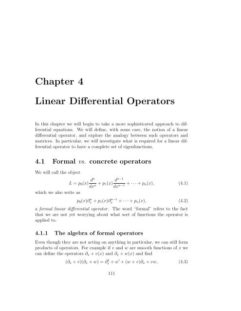
Chapter 4 Linear Differential Operators

Chapter 4
Linear Differential Operators
In this chapter we will begin to take a more sophisticated approach to differential
equations. We will define, with some care, the notion of a linear
differential operator, and explore the analogy between such operators and
matrices. In particular, we will investigate what is required for a linear differential
operator to have a complete set of eigenfunctions.
4.1 Formal vs. concrete operators
We will call the object
L = p0(x) dn dn−1
+ p1(x)
dxn dxn−1 + · · · + pn(x), (4.1)
which we also write as
p0(x)∂ n x + p1(x)∂ n−1
x + · · · + pn(x), (4.2)
a formal linear differential operator. The word “formal” refers to the fact
that we are not yet worrying about what sort of functions the operator is
applied to.
4.1.1 The algebra of formal operators
Even though they are not acting on anything in particular, we can still form
products of operators. For example if v and w are smooth functions of x we
can define the operators ∂x + v(x) and ∂x + w(x) and find
(∂x + v)(∂x + w) = ∂ 2 x + w′ + (w + v)∂x + vw, (4.3)
111

112 CHAPTER 4. LINEAR DIFFERENTIAL OPERATORS
or
(∂x + w)(∂x + v) = ∂ 2 x + v ′ + (w + v)∂x + vw, (4.4)
We see from this example that the operator algebra is not usually commutative.
The algebra of formal operators has some deep applications. Consider,
for example, the operators
and
L = −∂ 2 x + q(x) (4.5)
P = ∂ 3 x + a(x)∂x + ∂xa(x). (4.6)
In the last expression, the combination ∂xa(x) means “first multiply by a(x),
and then differentiate the result,” so we could also write
∂xa = a∂x + a ′ . (4.7)
We can now form the commutator [P, L] ≡ P L − LP . After a little effort,
we find
[P, L] = (3q ′ + 4a ′ )∂ 2 x + (3q′′ + 4a ′′ )∂x + q ′′′ + 2aq ′ + a ′′′ . (4.8)
If we choose a = − 3
q, the commutator becomes a pure multiplication oper-
4
ator, with no differential part:
The equation
or, equivalently,
has a formal solution
[P, L] = 1
4 q′′′ − 3
2 qq′ . (4.9)
dL
dt
= [P, L], (4.10)
˙q = 1
4 q′′′ − 3
2 qq′ , (4.11)
L(t) = e tP L(0)e −tP , (4.12)
showing that the time evolution of L is given by a similarity transformation,
which (again formally) does not change its eigenvalues. The partial differential
equation (4.11) is the famous Korteweg de Vries (KdV) equation, which
has “soliton” solutions whose existence is intimately connected with the fact
that it can be written as (4.10). The operators P and L are called a Lax
pair, after Peter Lax who uncovered much of the structure.

4.1. FORMAL VS. CONCRETE OPERATORS 113
4.1.2 Concrete operators
We want to explore the analogies between linear differential operators and
matrices acting on a finite-dimensional vector space. Because the theory of
matrix operators makes much use of inner products and orthogonality, the
analogy is closest if we work with a function space equipped with these same
notions. We therefore let our differential operators act on L 2 [a, b], the Hilbert
space of square-integrable functions on [a, b]. Now a differential operator
cannot act on every function in the Hilbert space because not all of them
are differentiable. Even though we will relax our notion of differentiability
and permit weak derivatives, we must at least demand that the domain D,
the subset of functions on which we allow the operator to act, contain only
functions that are sufficiently differentiable that the function resulting from
applying the operator remains an element of L 2 [a, b]. We will usually restrict
the set of functions even further, by imposing boundary conditions at the
endpoints of the interval. A linear differential operator is now defined as a
formal linear differential operator, together with a specification of its domain
D.
The boundary conditions that we will impose will always be linear and
homogeneous. This is so that the domain of definition is a vector space.
In other words, if y1 and y2 obey the boundary conditions then so should
λy1 + µy2. Thus, for a second-order operator
L = p0∂ 2 x + p1∂x + p2
on the interval [a, b], we might impose
B1[y] = α11y(a) + α12y ′ (a) + β11y(b) + β12y ′ (b) = 0,
(4.13)
B2[y] = α21y(a) + α22y ′ (a) + β21y(b) + β22y ′ (b) = 0, (4.14)
but we will not, in defining the differential operator, impose inhomogeneous
conditions, such as
B1[y] = α11y(a) + α12y ′ (a) + β11y(b) + β12y ′ (b) = A,
B2[y] = α21y(a) + α22y ′ (a) + β21y(b) + β22y ′ (b) = B, (4.15)
with non-zero A, B — even though we will solve differential equations with
such boundary conditions.

114 CHAPTER 4. LINEAR DIFFERENTIAL OPERATORS
Also, for an n-th order operator, we will not constrain derivatives of order
higher than n − 1. This is reasonable 1 : If we seek solutions of Ly = f with L
a second-order operator, for example, then the values of y ′′ at the endpoints
are already determined in terms of y ′ and y by the differential equation. We
cannot choose to impose some other value. By differentiating the equation
enough times, we can similarly determine all higher endpoint derivatives in
terms of y and y ′ . These two derivatives, therefore, are all we can fix by fiat.
The boundary and differentiability conditions that we impose make D a
subset of the entire Hilbert space. This subset will always be dense: any
element of the Hilbert space can be obtained as an L 2 limit of functions in
D. In particular, there will never be a function in L 2 [a, b] that is orthogonal
to all functions in D.
4.2 The adjoint operator
One of the important properties of matrices, established in the appendix,
is that a matrix that is self-adjoint, or Hermitian, may be diagonalized. In
other words, the matrix has sufficiently many eigenvectors for them to form
a basis for the space on which it acts. A similar property holds for selfadjoint
differential operators, but we must be careful in our definition of
self-adjointness.
Before reading this section, We suggest you review the material on adjoint
operators on finite-dimensional spaces that appears in the appendix.
4.2.1 The formal adjoint
Given a formal differential operator
L = p0(x) dn dn−1
+ p1(x)
dxn dxn−1 + · · · + pn(x), (4.16)
and a weight function w(x), real and positive on the interval (a, b), we can
find another such operator L † , such that, for any sufficiently differentiable
u(x) and v(x), we have
w u ∗ Lv − v(L † u) ∗ = d
Q[u, v], (4.17)
dx
1 There is a deeper reason which we will explain in section 9.7.2.

4.2. THE ADJOINT OPERATOR 115
for some function Q, which depends bilinearly on u and v and their first n−1
derivatives. We call L † the formal adjoint of L with respect to the weight w.
The equation (4.17) is called Lagrange’s identity. The reason for the name
“adjoint” is that if we define an inner product
〈u, v〉 w =
b
a
wu ∗ v dx, (4.18)
and if the functions u and v have boundary conditions that make Q[u, v]| b a =
0, then
〈u, Lv〉 w = 〈L † u, v〉 w , (4.19)
which is the defining property of the adjoint operator on a vector space. The
word “formal” means, as before, that we are not yet specifying the domain
of the operator.
The method for finding the formal adjoint is straightforward: integrate
by parts enough times to get all the derivatives off v and on to u.
Example: If
L = −i d
(4.20)
dx
then let us find the adjoint L † with respect to the weight w ≡ 1. We start
from
u ∗ (Lv) = u ∗
−i d
dx v
,
and use the integration-by-parts technique once to get the derivative off v
and onto u∗ :
u ∗
−i d
dx v
= i d
dx u∗
v − i d
dx (u∗v)
= −i d
dx u
∗ v − i d
dx (u∗v) We have ended up with the Lagrange identity
u ∗
≡ v(L † u) ∗ + d
Q[u, v]. (4.21)
dx
−i d
dx v
− v
−i d
dx u
∗
= d
dx (−iu∗ v), (4.22)

116 CHAPTER 4. LINEAR DIFFERENTIAL OPERATORS
and found that
L † = −i d
dx , Q[u, v] = −iu∗v. (4.23)
The operator −id/dx (which you should recognize as the “momentum” operator
from quantum mechanics) obeys L = L † , and is therefore, formally
self-adjoint, or Hermitian.
Example: Let
d
L = p0
2 d
+ p1
dx2 dx + p2, (4.24)
with the pi all real. Again let us find the adjoint L † with respect to the inner
product with w ≡ 1. Now, proceeding as above, but integrating by parts
twice, we find
u ∗ [p0v ′′ + p1v ′ + p2v] − v [(p0u) ′′ − (p1u) ′ + p2u] ∗
= d
p0(u
dx
∗ v ′ − vu ∗′ ) + (p1 − p ′ 0 )u∗v . (4.25)
From this we read off that
L † = d2
dx2 p0 − d
dx p1 + p2
= p0
d 2
dx 2 + (2p′ 0
d
− p1) + (p′′ 0
dx − p′ 1 + p2). (4.26)
What conditions do we need to impose on p0,1,2 for this L to be formally
self-adjoint with respect to the inner product with w ≡ 1? For L = L † we
need
We therefore require that p1 = p ′ 0
p0 = p0
2p ′ 0 − p1 = p1 ⇒ p ′ 0 = p1
p ′′
0 − p ′ 1 + p2 = p2 ⇒ p ′′
0 = p ′ 1. (4.27)
, and so
L = d
d
p0 + p2, (4.28)
dx dx
which we recognize as a Sturm-Liouville operator.
Example: Reduction to Sturm-Liouville form. Another way to make the
operator
d
L = p0
2 d
+ p1
dx2 dx + p2, (4.29)

4.2. THE ADJOINT OPERATOR 117
self-adjoint is by a suitable choice of weight function w. Suppose that p0 is
positive on the interval (a, b), and that p0, p1, p2 are all real. Then we may
define
w = 1
x
p1
exp
dx ′
(4.30)
and observe that it is positive on (a, b), and that
Now
where
p0
a
p0
Ly = 1
w (wp0y ′ ) ′ + p2y. (4.31)
〈u, Lv〉 w − 〈Lu, v〉 w = [wp0(u ∗ v ′ − u ∗′ v)] b a , (4.32)
〈u, v〉 w =
b
a
wu ∗ v dx. (4.33)
Thus, provided p0 does not vanish, there is always some inner product with
respect to which a real second-order differential operator is formally selfadjoint.
Note that with
Ly = 1
w (wp0y ′ ) ′ + p2y, (4.34)
the eigenvalue equation
Ly = λy (4.35)
can be written
(wp0y ′ ) ′ + p2wy = λwy. (4.36)
When you come across a differential equation where, in the term containing
the eigenvalue λ, the eigenfunction is being multiplied by some other function,
you should immediately suspect that the operator will turn out to be selfadjoint
with respect to the inner product having this other function as its
weight.
Illustration (Bargmann-Fock space): This is a more exotic example of a
formal adjoint. You may have met with it in quantum mechanics. Consider
the space of polynomials P (z) in the complex variable z = x + iy. Define an
inner product by
〈P, Q〉 = 1
d
π
2 z e −z∗z ∗
[P (z)] Q(z),

118 CHAPTER 4. LINEAR DIFFERENTIAL OPERATORS
where d 2 z ≡ dx dy and the integration is over the entire x, y plane. With
this inner product, we have
If we define
then
〈P, â Q〉 = 1
π
= − 1
π
= 1
π
= 1
π
〈z n , z m 〉 = n!δnm.
= 〈â † P, ˆ Q〉
â = d
dz ,
d 2 z e −z∗ z [P (z)] ∗ d
dz Q(z)
d 2
d
z
dz e−z∗
z ∗
[P (z)] Q(z)
d 2 z e −z∗ z z ∗ [P (z)] ∗ Q(z)
d 2 z e −z∗ z [zP (z)] ∗ Q(z)
where â † = z, i.e. the operation of multiplication by z. In this case, the
adjoint is not even a differential operator. 2
Exercise 4.1: Consider the differential operator ˆ L = id/dx. Find the formal
adjoint of L with respect to the inner product 〈u, v〉 = wu ∗ v dx, and find
the corresponding surface term Q[u, v].
2 In deriving this result we have used the Wirtinger calculus where z and z ∗ are treated
as independent variables so that
d
dz e−z∗ z = −z ∗ e −z ∗ z ,
and observed that, because [P (z)] ∗ is a function of z ∗ only,
d
dz [P (z)]∗ = 0.
If you are uneasy at regarding z, z∗ , as independent, you should confirm these formulae
by expressing z and z∗ in terms of x and y, and using
d 1 ∂ ∂ d 1 ∂ ∂
≡ − i , ≡ + i .
dz 2 ∂x ∂y dz∗ 2 ∂x ∂y

4.2. THE ADJOINT OPERATOR 119
Exercise 4.2:Sturm-Liouville forms. By constructing appropriate weight functions
w(x) convert the following common operators into Sturm-Liouville form:
a) ˆ L = (1 − x 2 ) d 2 /dx 2 + [(µ − ν) − (µ + ν + 2)x] d/dx.
b) ˆ L = (1 − x 2 ) d 2 /dx 2 − 3x d/dx.
c) ˆ L = d 2 /dx 2 − 2x(1 − x 2 ) −1 d/dx − m 2 (1 − x 2 ) −1 .
4.2.2 A simple eigenvalue problem
A finite Hermitian matrix has a complete set of orthonormal eigenvectors.
Does the same property hold for a Hermitian differential operator?
Consider the differential operator
T = −∂ 2 x, D(T ) = {y, T y ∈ L 2 [0, 1] : y(0) = y(1) = 0}. (4.37)
With the inner product
we have
〈y1, y2〉 =
1
y
0
∗ 1y2 dx (4.38)
〈y1, T y2〉 − 〈T y1, y2〉 = [y ′ ∗
1 y2 − y ∗ 1y ′ 2] 1 0 = 0. (4.39)
The integrated-out part is zero because both y1 and y2 satisfy the boundary
conditions. We see that
〈y1, T y2〉 = 〈T y1, y2〉 (4.40)
and so T is Hermitian or symmetric.
The eigenfunctions and eigenvalues of T are
n = 1, 2, . . . . (4.41)
yn(x) = sin nπx
λn = n 2 π 2
We see that:
i) the eigenvalues are real;
ii) the eigenfunctions for different λn are orthogonal,
1
2 sin nπx sin mπx dx = δnm, n = 1, 2, . . . (4.42)
0

120 CHAPTER 4. LINEAR DIFFERENTIAL OPERATORS
iii) the normalized eigenfunctions ϕn(x) = √ 2 sin nπx are complete: any
function in L 2 [0, 1] has an (L 2 ) convergent expansion as
where
y(x) =
an =
1
0
∞
n=1
√
an 2 sin nπx (4.43)
y(x) √ 2 sin nπx dx. (4.44)
This all looks very good — exactly the properties we expect for finite Hermitian
matrices. Can we carry over all the results of finite matrix theory to
these Hermitian operators? The answer sadly is no! Here is a counterexample:
Let
Again
T = −i∂x, D(T ) = {y, T y ∈ L 2 [0, 1] : y(0) = y(1) = 0}. (4.45)
〈y1, T y2〉 − 〈T y1, y2〉 =
1
0
dx {y ∗ 1 (−i∂xy2) − (−i∂xy1) ∗ y2}
= −i[y ∗ 1y2] 1 0 = 0. (4.46)
Once more, the integrated out part vanishes due to the boundary conditions
satisfied by y1 and y2, so T is nicely Hermitian. Unfortunately, T with these
boundary conditions has no eigenfunctions at all — never mind a complete
set! Any function satisfying T y = λy will be proportional to e iλx , but an exponential
function is never zero, and cannot satisfy the boundary conditions.
It seems clear that the boundary conditions are the problem. We need
a better definition of “adjoint” than the formal one — one that pays more
attention to boundary conditions. We will then be forced to distinguish
between mere Hermiticity, or symmetry, and true self-adjointness.
Exercise 4.3: Another disconcerting example. Let p = −i∂x. Show that the
following operator on the infinite real line is formally self-adjoint:
Now let
H = x 3 p + px 3 . (4.47)
ψλ(x) = |x| −3/2
exp − λ
4x2
, (4.48)

4.2. THE ADJOINT OPERATOR 121
where λ is real and positive. Show that
Hψλ = −iλψλ, (4.49)
so ψλ is an eigenfunction with a purely imaginary eigenvalue. Examine the
proof that Hermitian operators have real eigenvalues, and identify at which
point it fails. (Hint: H is formally self adjoint because it is of the form T +T † .
Now ψλ is square-integrable, and so an element of L 2 (R). Is T ψλ an element
of L 2 (R)?)
4.2.3 Adjoint boundary conditions
The usual definition of the adjoint operator in linear algebra is as follows:
Given the operator T : V → V and an inner product 〈 , 〉, we look at
〈u, T v〉, and ask if there is a w such that 〈w, v〉 = 〈u, T v〉 for all v. If there
is, then u is in the domain of T † , and we set T † u = w.
For finite-dimensional vector spaces V there always is such a w, and so
the domain of T † is the entire space. In an infinite dimensional Hilbert space,
however, not all 〈u, T v〉 can be written as 〈w, v〉 with w a finite-length element
of L 2 . In particular δ-functions are not allowed — but these are exactly what
we would need if we were to express the boundary values appearing in the
integrated out part, Q(u, v), as an inner-product integral. We must therefore
ensure that u is such that Q(u, v) vanishes, but then accept any u with this
property into the domain of T † . What this means in practice is that we look
at the integrated out term Q(u, v) and see what is required of u to make
Q(u, v) zero for any v satisfying the boundary conditions appearing in D(T ).
These conditions on u are the adjoint boundary conditions, and define the
domain of T † .
Example: Consider
Now,
1
0
T = −i∂x, D(T ) = {y, T y ∈ L 2 [0, 1] : y(1) = 0}. (4.50)
dx u ∗ (−i∂xv) = −i[u ∗ (1)v(1) − u ∗ (0)v(0)] +
1
0
dx(−i∂xu) ∗ v
= −i[u ∗ (1)v(1) − u ∗ (0)v(0)] + 〈w, v〉, (4.51)
where w = −i∂xu. Since v(x) is in the domain of T , we have v(1) = 0, and
so the first term in the integrated out bit vanishes whatever value we take

122 CHAPTER 4. LINEAR DIFFERENTIAL OPERATORS
for u(1). On the other hand, v(0) could be anything, so to be sure that the
second term vanishes we must demand that u(0) = 0. This, then, is the
adjoint boundary condition. It defines the domain of T † :
T † = −i∂x, D(T † ) = {y, T y ∈ L 2 [0, 1] : y(0) = 0}. (4.52)
For our problematic operator
we have
T = −i∂x, D(T ) = {y, T y ∈ L 2 [0, 1] : y(0) = y(1) = 0}, (4.53)
1
0
dx u ∗ (−i∂xv) = −i[u ∗ v] 1 0 +
1
0
dx(−i∂xu) ∗ v
= 0 + 〈w, v〉, (4.54)
where again w = −i∂xu. This time no boundary conditions need be imposed
on u to make the integrated out part vanish. Thus
T † = −i∂x, D(T † ) = {y, T y ∈ L 2 [0, 1]}. (4.55)
Although any of these operators “T = −i∂x” is formally self-adjoint we
have,
D(T ) = D(T † ), (4.56)
so T and T † are not the same operator and none of them is truly self-adjoint.
Exercise 4.4: Consider the differential operator M = d 4 /dx 4 , Find the formal
adjoint of M with respect to the inner product 〈u, v〉 = u ∗ v dx, and find
the corresponding surface term Q[u, v]. Find the adjoint boundary conditions
defining the domain of M † for the case
D(M) = {y, y (4) ∈ L 2 [0, 1] : y(0) = y ′′′ (0) = y(1) = y ′′′ (1) = 0}.
4.2.4 Self-adjoint boundary conditions
A formally self-adjoint operator T is truly self adjoint only if the domains of
T † and T coincide. From now on, the unqualified phrase “self-adjoint” will
always mean “truly self-adjoint.”
Self-adjointness is usually desirable in physics problems. It is therefore
useful to investigate what boundary conditions lead to self-adjoint operators.

4.2. THE ADJOINT OPERATOR 123
For example, what are the most general boundary conditions we can impose
on T = −i∂x if we require the resultant operator to be self-adjoint? Now,
1
0
dx u ∗ (−i∂xv) −
1
0
dx(−i∂xu) ∗
v = −i u ∗ (1)v(1) − u ∗
(0)v(0) . (4.57)
Demanding that the right-hand side be zero gives us, after division by u ∗ (0)v(1),
u ∗ (1)
u ∗ (0)
v(0)
= . (4.58)
v(1)
We require this to be true for any u and v obeying the same boundary
conditions. Since u and v are unrelated, both sides must equal a constant κ,
and furthermore this constant must obey κ ∗ = κ −1 in order that u(1)/u(0)
be equal to v(1)/v(0). Thus, the boundary condition is
u(1) v(1)
= = eiθ
u(0) v(0)
for some real angle θ. The domain is therefore
(4.59)
D(T ) = {y, T y ∈ L 2 [0, 1] : y(1) = e iθ y(0)}. (4.60)
These are twisted periodic boundary conditions.
With these generalized periodic boundary conditions, everything we expect
of a self-adjoint operator actually works:
i) The functions un = e i(2πn+θ)x , with n = . . . , −2, −1, 0, 1, 2 . . . are eigenfunctions
of T with eigenvalues kn ≡ 2πn + θ.
ii) The eigenvalues are real.
iii) The eigenfunctions form a complete orthonormal set.
Because self-adjoint operators possess a complete set of mutually orthogonal
eigenfunctions, they are compatible with the interpretational postulates
of quantum mechanics, where the square of the inner product of a state
vector with an eigenstate gives the probability of measuring the associated
eigenvalue. In quantum mechanics, self-adjoint operators are therefore called
observables.
Example: The Sturm-Liouville equation. With
L = d d
p(x) + q(x), x ∈ [a, b], (4.61)
dx dx

124 CHAPTER 4. LINEAR DIFFERENTIAL OPERATORS
we have
〈u, Lv〉 − 〈Lu, v〉 = [p(u ∗ v ′ − u ′∗ v)] b a . (4.62)
Let us seek to impose boundary conditions separately at the two ends. Thus,
at x = a we want
(u ∗ v ′ − u ′∗ v)|a = 0, (4.63)
or
u ′∗
(a)
u∗ (a) = v′ (a)
, (4.64)
v(a)
and similarly at b. If we want the boundary conditions imposed on v (which
define the domain of L) to coincide with those for u (which define the domain
of L † ) then we must have
v ′ (a)
v(a) = u′ (a)
= tan θa
(4.65)
u(a)
for some real angle θa, and similar boundary conditions with a θb at b. We
can also write these boundary conditions as
αay(a) + βay ′ (a) = 0,
αby(b) + βby ′ (b) = 0. (4.66)
Deficiency indices and self-adjoint extensions
There is a general theory of self-adjoint boundary conditions, due to Hermann
Weyl and John von Neumann. We will not describe this theory in any
detail, but simply give their recipe for counting the number of parameters
in the most general self-adjoint boundary condition: To find this number we
define an initial domain D0(L) for the operator L by imposing the strictest
possible boundary conditions. This we do by setting to zero the boundary
values of all the y (n) with n less than the order of the equation. Next
count the number of square-integrable eigenfunctions of the resulting adjoint
operator T † corresponding to eigenvalue ±i. The numbers, n+ and n−, of
these eigenfunctions are called the deficiency indices. If they are not equal
then there is no possible way to make the operator self-adjoint. If they are
equal, n+ = n− = n, then there is an n 2 real-parameter family of self-adjoint
extensions D(L) ⊃ D0(L) of the initial tightly-restricted domain.

4.2. THE ADJOINT OPERATOR 125
Example: The sad case of the “radial momentum operator.” We wish to
define the operator Pr = −i∂r on the half-line 0 < r < ∞. We start with the
restrictive domain
We then have
Pr = −i∂r, D0(T ) = {y, Pry ∈ L 2 [0, ∞] : y(0) = 0}. (4.67)
P † r = −i∂r, D(P † r ) = {y, P † r y ∈ L2 [0, ∞]} (4.68)
with no boundary conditions. The equation P † r y = iy has a normalizable
solution y = e−r . The equation P † r y = −iy has no normalizable solution.
The deficiency indices are therefore n+ = 1, n− = 0, and this operator
cannot be rescued and made self adjoint.
Example: The Schrödinger operator. We now consider −∂ 2 x on the half-line.
Set
T = −∂ 2 x, D0(T ) = {y, T y ∈ L 2 [0, ∞] : y(0) = y ′ (0) = 0}. (4.69)
We then have
T † = −∂ 2 x , D(T † ) = {y, T † y ∈ L 2 [0, ∞]}. (4.70)
Again T † comes with no boundary conditions. The eigenvalue equation
T † y = iy has one normalizable solution y(x) = e (i−1)x/√2 , and the equation
T † y = −iy also has one normalizable solution y(x) = e−(i+1)x/√2 . The deficiency
indices are therefore n+ = n− = 1. The Weyl-von Neumann theory
now says that, by relaxing the restrictive conditions y(0) = y ′ (0) = 0, we
can extend the domain of definition of the operator to find a one-parameter
family of self-adjoint boundary conditions. These will be the conditions
y ′ (0)/y(0) = tan θ that we found above.
If we consider the operator −∂ 2 x
on the finite interval [a, b], then both
solutions of (T † ± i)y = 0 are normalizable, and the deficiency indices will
be n+ = n− = 2. There should therefore be 2 2 = 4 real parameters in the
self-adjoint boundary conditions. This is a larger class than those we found
in (4.66), because it includes generalized boundary conditions of the form
B1[y] = α11y(a) + α12y ′ (a) + β11y(b) + β12y ′ (b) = 0,
B2[y] = α21y(a) + α22y ′ (a) + β21y(b) + β22y ′ (b) = 0

126 CHAPTER 4. LINEAR DIFFERENTIAL OPERATORS
GaAs: m L
ψ ψ
L R
?
AlGaAs:m R
Figure 4.1: Heterojunction and wavefunctions.
Physics application: semiconductor heterojunction
We now demonstrate why we have spent so much time on identifying selfadjoint
boundary conditions: the technique is important in practical physics
problems.
A heterojunction is an atomically smooth interface between two related
semiconductors, such as GaAs and AlxGa1−xAs, which typically possess different
band-masses. We wish to describe the conduction electrons by an
effective Schrödinger equation containing these band masses. What matching
condition should we impose on the wavefunction ψ(x) at the interface
between the two materials? A first guess is that the wavefunction must be
continuous, but this is not correct because the “wavefunction” in an effectivemass
band-theory Hamiltonian is not the actual wavefunction (which is continuous)
but instead a slowly varying envelope function multiplying a Bloch
wavefunction. The Bloch function is rapidly varying, fluctuating strongly
on the scale of a single atom. Because the Bloch form of the solution is no
longer valid at a discontinuity, the envelope function is not even defined in
the neighbourhood of the interface, and certainly has no reason to be continuous.
There must still be some linear relation beween the ψ’s in the two
materials, but finding it will involve a detailed calculation on the atomic
scale. In the absence of these calculations, we must use general principles to
constrain the form of the relation. What are these principles?
We know that, were we to do the atomic-scale calculation, the resulting
connection between the right and left wavefunctions would:
• be linear,
• involve no more than ψ(x) and its first derivative ψ ′ (x),
• make the Hamiltonian into a self-adjoint operator.
We want to find the most general connection formula compatible with these
x

4.2. THE ADJOINT OPERATOR 127
principles. The first two are easy to satisfy. We therefore investigate what
matching conditions are compatible with self-adjointness.
Suppose that the band masses are mL and mR, so that
H = − 1 d
2mL
2
dx2 + VL(x), x < 0,
= − 1
2mR
d 2
dx 2 + VR(x), x > 0. (4.71)
Integrating by parts, and keeping the terms at the interface gives us
〈ψ1, Hψ2〉−〈Hψ1, ψ2〉 = 1
2mL
ψ ∗ 1L ψ ′ 2L
− ψ′∗1Lψ2L
1
∗
− ψ1Rψ 2mR
′ 2R − ψ′∗ 1Rψ2R
.
(4.72)
Here, ψL,R refers to the boundary values of ψ immediately to the left or right
of the junction, respectively. Now we impose general linear homogeneous
boundary conditions on ψ2:
ψ2L
ψ ′
a
=
2L c
b ψ2R
d ψ ′
.
2R
(4.73)
This relation involves four complex, and therefore eight real, parameters.
Demanding that
〈ψ1, Hψ2〉 = 〈Hψ1, ψ2〉, (4.74)
we find
1 ∗
ψ1L (cψ2R + dψ
2mL
′ 2R ) − ψ′∗1L
(aψ2R + bψ ′ 2R ) = 1 ∗
ψ1Rψ 2mR
′ 2R − ψ′∗1Rψ2R
,
(4.75)
and this must hold for arbitrary ψ2R, ψ ′ 2R , so, picking off the coefficients of
these expressions and complex conjugating, we find
ψ1R mR
∗ ∗ d −b
=
−c∗ a∗
ψ1L
. (4.76)
ψ ′ 1R
mL
Because we wish the domain of H † to coincide with that of H, these must
be same conditions that we imposed on ψ2. Thus we must have
−1 a b
=
c d
mR
mL
d ∗ −b ∗
−c ∗ a ∗
ψ ′ 1L
. (4.77)

128 CHAPTER 4. LINEAR DIFFERENTIAL OPERATORS
Since −1 a b
=
c d
1 d −b
, (4.78)
ad − bc −c a
we see that this requires
a
c
b
= e
d
iφ
mL A
mR C
B
,
D
(4.79)
where φ, A, B, C, D are real, and AD−BC = 1. Demanding self-adjointness
has therefore cut the original eight real parameters down to four. These
can be determined either by experiment or by performing the microscopic
calculation. 3 Note that 4 = 2 2 , a perfect square, as required by the Weyl-
Von Neumann theory.
Exercise 4.5: Consider the Schrödinger operator ˆ H = −∂ 2 x on the interval
[0, 1]. Show that the most general self-adjoint boundary condition applicable
to ˆ H can be written as
ϕ(0)
ϕ ′
= e
(0)
iφ
a b ϕ(1)
c d ϕ ′
,
(1)
where φ, a, b, c, d are real and ac − bd = 1. Consider ˆ H as the quantum
Hamiltonian of a particle on a ring constructed by attaching x = 0 to x = 1.
Show that the self-adjoint boundary condition found above leads to unitary
scattering at the point of join. Does the most general unitary point-scattering
matrix correspond to the most general self-adjoint boundary condition?
4.3 Completeness of eigenfunctions
Now that we have a clear understanding of what it means to be self-adjoint,
we can reiterate the basic claim: an operator T that is self-adjoint with
respect to an L 2 [a, b] inner product possesses a complete set of mutually orthogonal
eigenfunctions. The proof that the eigenfunctions are orthogonal
is identical to that for finite matrices. We will sketch a proof of the completeness
of the eigenfunctions of the Sturm-Liouville operator in the next
section.
The set of eigenvalues is, with some mathematical cavils, called the spectrum
of T . It is usually denoted by σ(T ). An eigenvalue is said to belong to
3 For example, see: T. Ando, S. Mori, Surface Science 113 (1982) 124.

4.3. COMPLETENESS OF EIGENFUNCTIONS 129
the point spectrum when its associated eigenfunction is normalizable i.e is
a bona-fide member of L 2 [a, b] having a finite length. Usually (but not always)
the eigenvalues of the point spectrum form a discrete set, and so the
point spectrum is also known as the discrete spectrum. When the operator
acts on functions on an infinite interval, the eigenfunctions may fail to
be normalizable. The associated eigenvalues are then said to belong to the
continuous spectrum. Sometimes, e.g. the hydrogen atom, the spectrum is
partly discrete and partly continuous. There is also something called the
residual spectrum, but this does not occur for self-adjoint operators.
4.3.1 Discrete spectrum
The simplest problems have a purely discrete spectrum. We have eigenfunctions
φn(x) such that
T φn(x) = λnφn(x), (4.80)
where n is an integer. After multiplication by suitable constants, the φn are
orthonormal,
φ ∗ n(x)φm(x) dx = δnm, (4.81)
and complete. We can express the completeness condition as the statement
that
φn(x)φ ∗ n (x′ ) = δ(x − x ′ ). (4.82)
n
If we take this representation of the delta function and multiply it by f(x ′ )
and integrate over x ′ , we find
f(x) =
φn(x) φ ∗ n(x ′ )f(x ′ ) dx ′ . (4.83)
So,
with
n
f(x) =
anφn(x) (4.84)
an =
n
φ ∗ n (x′ )f(x ′ ) dx ′ . (4.85)
This means that if we can expand a delta function in terms of the φn(x), we
can expand any (square integrable) function.

130 CHAPTER 4. LINEAR DIFFERENTIAL OPERATORS
60
40
20
0.2 0.4 0.6 0.8 1
Figure 4.2: The sum 70
n=1 2 sin(nπx) sin(nπx′ ) for x ′ = 0.4. Take note of
the very disparate scales on the horizontal and vertical axes.
Warning: The convergence of the series
n φn(x)φ ∗ n (x′ ) to δ(x − x ′ ) is
neither pointwise nor in the L 2 sense. The sum tends to a limit only in the
sense of a distribution — meaning that we must multiply the partial sums by
a smooth test function and integrate over x before we have something that
actually converges in any meaningful manner. As an illustration consider our
favourite orthonormal set: φn(x) = √ 2 sin(nπx) on the interval [0, 1]. A plot
of the first 70 terms in the sum
∞ √ √
′ ′
2 sin(nπx) 2 sin(nπx ) = δ(x − x )
n=1
is shown in figure 4.2. The “wiggles” on both sides of the spike at x =
x ′ do not decrease in amplitude as the number of terms grows. They do,
however, become of higher and higher frequency. When multiplied by a
smooth function and integrated, the contributions from adjacent positive and
negative wiggle regions tend to cancel, and it is only after this integration
that the sum tends to zero away from the spike at x = x ′ .
Rayleigh-Ritz and completeness
For the Schrödinger eigenvalue problem
Ly = −y ′′ + q(x)y = λy, x ∈ [a, b], (4.86)

4.3. COMPLETENESS OF EIGENFUNCTIONS 131
the large eigenvalues are λn ≈ n 2 π 2 /(a − b) 2 . This is because the term qy
eventually becomes negligeable compared to λy, and we can then solve the
equation with sines and cosines. We see that there is no upper limit to
the magnitude of the eigenvalues. The eigenvalues of the Sturm-Liouville
problem
Ly = −(py ′ ) ′ + qy = λy, x ∈ [a, b], (4.87)
are similarly unbounded. We will use this unboundedness of the spectrum to
make an estimate of the rate of convergence of the eigenfunction expansion
for functions in the domain of L, and extend this result to prove that the
eigenfunctions form a complete set.
We know from chapter one that the Sturm-Liouville eigenvalues are the
stationary values of 〈y, Ly〉 when the function y is constrained to have unit
length, 〈y, y〉 = 1. The lowest eigenvalue, λ0, is therefore given by
λ0 = inf
y∈D(L)
〈y, Ly〉
. (4.88)
〈y, y〉
As the variational principle, this formula provides a well-known method of
obtaining approximate ground state energies in quantum mechanics. Part of
its effectiveness comes from the stationary nature of 〈y, Ly〉 at the minimum:
a crude approximation to y often gives a tolerably good approximation to λ0.
In the wider world of eigenvalue problems, the variational principle is named
after Rayleigh and Ritz. 4
Suppose we have already found the first n normalized eigenfunctions
y0, y1, . . . , yn−1. Let the space spanned by these functions be Vn. Then an
obvious extension of the variational principle gives
λn = inf
y∈V ⊥ n
〈y, Ly〉
. (4.89)
〈y, y〉
We now exploit this variational estimate to show that if we expand an arbitrary
y in the domain of L in terms of the full set of eigenfunctions ym,
y =
∞
amym, (4.90)
m=0
4 J. W. Strutt (later Lord Rayleigh), “In Finding the Correction for the Open End of
an Organ-Pipe.” Phil. Trans. 161 (1870) 77; W. Ritz, ”Uber eine neue Methode zur
Lösung gewisser Variationsprobleme der mathematischen Physik.” J. reine angew. Math.
135 (1908).

132 CHAPTER 4. LINEAR DIFFERENTIAL OPERATORS
where
then the sum does indeed converge to y.
Let
am = 〈ym, y〉, (4.91)
hn = y −
n−1
m=0
amym
(4.92)
be the residual error after the first n terms. By definition, hn ∈ V ⊥ n . Let
us assume that we have adjusted, by adding a constant to q if necessary, L
so that all the λm are positive. This adjustment will not affect the ym. We
expand out
〈hn, Lhn〉 = 〈y, Ly〉 −
n−1
m=0
λm|am| 2 , (4.93)
where we have made use of the orthonormality of the ym. The subtracted
sum is guaranteed positive, so
〈hn, Lhn〉 ≤ 〈y, Ly〉. (4.94)
Combining this inequality with Rayleigh-Ritz tells us that
In other words
〈y, Ly〉
〈hn, hn〉 ≥ 〈hn, Lhn〉
〈hn, hn〉 ≥ λn. (4.95)
〈y, Ly〉
≥ y −
λn
n−1
m=0
amym 2 . (4.96)
Since 〈y, Ly〉 is independent of n, and λn → ∞, we have y − n−1 0 amym2 → 0.
Thus the eigenfunction expansion indeed converges to y, and does so faster
than λ −1
n goes to zero.
Our estimate of the rate of convergence applies only to the expansion of
functions y for which 〈y, Ly〉 is defined — i.e. to functions y ∈ D (L). The
domain D (L) is always a dense subset of the entire Hilbert space L 2 [a, b],
however, and, since a dense subset of a dense subset is also dense in the larger
space, we have shown that the linear span of the eigenfunctions is a dense
subset of L 2 [a, b]. Combining this observation with the alternative definition
of completeness in 2.2.3, we see that the eigenfunctions do indeed form a
complete orthonormal set. Any square integrable function therefore has a
convergent expansion in terms of the ym, but the rate of convergence may
well be slower than that for functions y ∈ D (L).

4.3. COMPLETENESS OF EIGENFUNCTIONS 133
Operator methods
Sometimes there are tricks for solving the eigenvalue problem.
Example: Quantum Harmonic Oscillator. Consider the operator
H = (−∂x + x)(∂x + x) + 1 = −∂ 2 x + x2 . (4.97)
This is in the form Q † Q + 1, where Q = (∂x + x), and Q † = (−∂x + x) is its
formal adjoint. If we write these operators in the opposite order we have
QQ † = (∂x + x)(−∂x + x) = −∂ 2 x + x 2 + 1 = H + 1. (4.98)
Now, if ψ is an eigenfunction of Q † Q with non-zero eigenvalue λ then Qψ is
eigenfunction of QQ † with the same eigenvalue. This is because
implies that
or
Q † Qψ = λψ (4.99)
Q(Q † Qψ) = λQψ, (4.100)
QQ † (Qψ) = λ(Qψ). (4.101)
The only way that Qψ can fail to be an eigenfunction of QQ † is if it happens
that Qψ = 0, but this implies that Q † Qψ = 0 and so the eigenvalue was zero.
Conversely, if the eigenvalue is zero then
0 = 〈ψ, Q † Qψ〉 = 〈Qψ, Qψ〉, (4.102)
and so Qψ = 0. In this way, we see that Q † Q and QQ † have exactly the
same spectrum, with the possible exception of any zero eigenvalue.
Now notice that Q † Q does have a zero eigenvalue because
1
−
ψ0 = e 2 x2
(4.103)
obeys Qψ0 = 0 and is normalizable. The operator QQ † , considered as an
operator on L 2 [−∞, ∞], does not have a zero eigenvalue because this would
require Q † ψ = 0, and so
1
+
ψ = e 2 x2
, (4.104)
which is not normalizable, and so not an element of L 2 [−∞, ∞].
Since
H = Q † Q + 1 = QQ † − 1, (4.105)

134 CHAPTER 4. LINEAR DIFFERENTIAL OPERATORS
we see that ψ0 is an eigenfunction of H with eigenvalue 1, and so an eigenfunction
of QQ † with eigenvalue 2. Hence Q † ψ0 is an eigenfunction of Q † Q
with eigenvalue 2 and so an eigenfunction H with eigenvalue 3. Proceeding
in the way we find that
ψn = (Q † ) n ψ0
is an eigenfunction of H with eigenvalue 2n + 1.
1
− ∂xe 2 x2,
we can write
where
Since Q † = −e 1
2 x2
(4.106)
1
−
ψn(x) = Hn(x)e 2 x2
, (4.107)
Hn(x) = (−1) n dn
x2
e
dx
n e−x2
(4.108)
are the Hermite Polynomials.
This is a useful technique for any second-order operator that can be factorized
— and a surprising number of the equations for “special functions”
can be. You will see it later, both in the exercises and in connection with
Bessel functions.
Exercise 4.6: Show that we have found all the eigenfunctions and eigenvalues
of H = −∂ 2 x + x 2 . Hint: Show that Q lowers the eigenvalue by 2 and use the
fact that Q † Q cannot have negative eigenvalues.
Problem 4.7: Schrödinger equations of the form
− d2 ψ
dx 2 − l(l + 1)sech2 x ψ = Eψ
are known as Pöschel-Teller equations. By setting u = ltanh x and following
the strategy of this problem one may relate solutions for l to those for l−1 and
so find all bound states and scattering eigenfunctions for any integer l.
a) Suppose that we know that ψ = exp − x
u(x ′ )dx ′ is a solution of
Lψ ≡ − d2
+ W (x) ψ = 0.
dx2 Show that L can be written as L = M † M where
d
M = + u(x) , M
dx †
= − d
+ u(x) ,
dx
the adjoint being taken with respect to the product 〈u, v〉 = u ∗ v dx.

4.3. COMPLETENESS OF EIGENFUNCTIONS 135
b) Now assume L is acting on functions on [−∞, ∞] and that we not have
to worry about boundary conditions. Show that given an eigenfunction
ψ− obeying M † Mψ− = λψ− we can multiply this equation on the left
by M and so find a eigenfunction ψ+ with the same eigenvalue for the
differential operator
L ′ = MM † =
d
+ u(x) −
dx d
+ u(x)
dx
and vice-versa. Show that this correspondence ψ− ↔ ψ+ will fail if, and
only if , λ = 0.
c) Apply the strategy from part b) in the case u(x) = tanh x and one of the
two differential operators M † M, MM † is (up to an additive constant)
H = − d
2
− 2 sech
dx
2 x.
Show that H has eigenfunctions of the form ψk = e ikx P (tanh x) and
eigenvalue E = k 2 for any k in the range −∞ < k < ∞. The function
P (tanh x) is a polynomial in tanh x which you should be able to find
explicitly. By thinking about the exceptional case λ = 0, show that H
has an eigenfunction ψ0(x), with eigenvalue E = −1, that tends rapidly
to zero as x → ±∞. Observe that there is no corresponding eigenfunction
for the other operator of the pair.
4.3.2 Continuous spectrum
Rather than a give formal discussion, we will illustrate this subject with some
examples drawn from quantum mechanics.
The simplest example is the free particle on the real line. We have
H = −∂ 2 x. (4.109)
We eventually want to apply this to functions on the entire real line, but we
will begin with the interval [−L/2, L/2], and then take the limit L → ∞
The operator H has formal eigenfunctions
ϕk(x) = e ikx , (4.110)
corresponding to eigenvalues λ = k 2 . Suppose we impose periodic boundary
conditions at x = ±L/2:
ϕk(−L/2) = ϕk(+L/2). (4.111)

136 CHAPTER 4. LINEAR DIFFERENTIAL OPERATORS
This selects kn = 2πn/L, where n is any positive, negative or zero integer,
and allows us to find the normalized eigenfunctions
The completeness condition is
∞
n=−∞
χn(x) = 1
√ L e iknx . (4.112)
1
L eiknx e −iknx′
= δ(x − x ′ ), x, x ′ ∈ [−L/2, L/2]. (4.113)
As L becomes large, the eigenvalues become so close that they can hardly be
distinguished; hence the name continuous spectrum, 5 and the spectrum σ(H)
becomes the entire positive real line. In this limit, the sum on n becomes an
integral
∞
n=−∞
. . . →
dn . . . =
dk
dn
. . . , (4.114)
dk
where
dn L
= (4.115)
dk 2π
is called the (momentum) density of states. If we divide this by L to get a
density of states per unit length, we get an L independent “finite” quantity,
the local density of states. We will often write
dn
dk
= ρ(k). (4.116)
If we express the density of states in terms of the eigenvalue λ then, by
an abuse of notation, we have
ρ(λ) ≡ dn
dλ
L
=
2π √ . (4.117)
λ
5 When L is strictly infinite, ϕk(x) is no longer normalizable. Mathematicians do not
allow such un-normalizable functions to be considered as true eigenfunctions, and so a
point in the continuous spectrum is not, to them, actually an eigenvalue. Instead, they
say that a point λ lies in the continuous spectrum if for any ɛ > 0 there exists an approximate
eigenfunction ϕɛ such that ϕɛ = 1, but Lϕɛ − λϕɛ < ɛ. This is not a
profitable definition for us. We prefer to regard non-normalizable wavefunctions as being
distributions in our rigged Hilbert space.

4.3. COMPLETENESS OF EIGENFUNCTIONS 137
Note that
dn
dλ
= 2dn
dk
dk
, (4.118)
dλ
which looks a bit weird, but remember that two states, ±kn, correspond to
the same λ and that the symbols
dn
dk ,
dn
dλ
(4.119)
are ratios of measures, i.e. Radon-Nikodym derivatives, not ordinary derivatives.
In the L → ∞ limit, the completeness condition becomes
∞
−∞
dk
2π eik(x−x′ ) = δ(x − x ′ ), (4.120)
and the length L has disappeared.
Suppose that we now apply boundary conditions y = 0 on x = ±L/2.
The normalized eigenfunctions are then
χn =
2
L sin kn(x + L/2), (4.121)
where kn = nπ/L. We see that the allowed k’s are twice as close together as
they were with periodic boundary conditions, but now n is restricted to being
a positive non-zero integer. The momentum density of states is therefore
ρ(k) = dn
dk
L
= , (4.122)
π
which is twice as large as in the periodic case, but the eigenvalue density of
states is
ρ(λ) = L
2π √ ,
λ
(4.123)
which is exactly the same as before.
That the number of states per unit energy per unit volume does not
depend on the boundary conditions at infinity makes physical sense: no
local property of the sublunary realm should depend on what happens in
the sphere of fixed stars. This point was not fully grasped by physicists,

138 CHAPTER 4. LINEAR DIFFERENTIAL OPERATORS
however, until Rudolph Peierls 6 explained that the quantum particle had to
actually travel to the distant boundary and back before the precise nature
of the boundary could be felt. This journey takes time T (depending on
the particle’s energy) and from the energy-time uncertainty principle, we
can distinguish one boundary condition from another only by examining the
spectrum with an energy resolution finer than /T . Neither the distance nor
the nature of the boundary can affect the coarse details, such as the local
density of states.
The dependence of the spectrum of a general differential operator on
boundary conditions was investigated by Hermann Weyl. Weyl distinguished
two classes of singular boundary points: limit-circle, where the spectrum
depends on the choice of boundary conditions, and limit-point, where it does
not. For the Schrödinger operator, the point at infinity, which is “singular”
simply because it is at infinity, is in the limit-point class. We will discuss
Weyl’s theory of singular endpoints in chapter 8.
Phase-shifts
Consider the eigenvalue problem
− d2
+ V (r) ψ = Eψ (4.124)
dr2 on the interval [0, R], and with boundary conditions ψ(0) = 0 = ψ(R). This
problem arises when we solve the Schrödinger equation for a central potential
in spherical polar coordinates, and assume that the wavefunction is a function
of r only (i.e. S-wave, or l = 0). Again, we want the boundary at R to be
infinitely far away, but we will start with R at a large but finite distance,
and then take the R → ∞ limit. Let us first deal with the simple case that
V (r) ≡ 0; then the solutions are
ψk(r) ∝ sin kr, (4.125)
with eigenvalue E = k2 , and with the allowed values of being given by
knR = nπ. Since
R
sin 2 (knr) dr = R
,
2
(4.126)
0
6 Peierls proved that the phonon contribution to the specific heat of a crystal could be
correctly calculated by using periodic boundary conditions. Some sceptics had thought
that such “unphysical” boundary conditions would give a result wrong by factors of two.

4.3. COMPLETENESS OF EIGENFUNCTIONS 139
the normalized wavefunctions are
2
ψk = sin kr,
R
and completeness reads
(4.127)
∞
2
sin(knr) sin(knr
R
′ ) = δ(r − r ′ ). (4.128)
n=1
As R becomes large, this sum goes over to an integral:
∞
2
sin(knr) sin(knr
R
n=1
′ ) →
∞
2
dn sin(kr) sin(kr
0 R
′ =
),
∞
Rdk 2
sin(kr) sin(kr
π R
′ ). (4.129)
Thus, ∞
2
dk sin(kr) sin(kr
π 0
′ ) = δ(r − r ′ ). (4.130)
As before, the large distance, here R, no longer appears.
Now consider the more interesting problem which has the potential V (r)
included. We will assume, for simplicity, that there is an R0 such that V (r)
is zero for r > R0. In this case, we know that the solution for r > R0 is of
the form
ψk(r) = sin (kr + η(k)) , (4.131)
where the phase shift η(k) is a functional of the potential V . The eigenvalue
is still E = k 2 .
Example: A delta-function shell. We take V (r) = λδ(r − a). See figure 4.3.
ψ
a
λδ (r−a)
Figure 4.3: Delta function shell potential.
0
r

140 CHAPTER 4. LINEAR DIFFERENTIAL OPERATORS
A solution with eigenvalue E = k2 and satisfying the boundary condition at
r = 0 is
A sin(kr), r < a,
ψ(r) =
(4.132)
sin(kr + η), r > a.
The conditions to be satisfied at r = a are:
i) continuity, ψ(a − ɛ) = ψ(a + ɛ) ≡ ψ(a), and
ii) jump in slope, −ψ ′ (a + ɛ) + ψ ′ (a − ɛ) + λψ(a) = 0.
Therefore,
ψ ′ (a + ɛ)
ψ(a) − ψ′ (a − ɛ)
= λ, (4.133)
ψ(a)
or
Thus,
and
−π
k cos(ka + η)
sin(ka + η)
− k cos(ka)
sin(ka)
= λ. (4.134)
cot(ka + η) − cot(ka) = λ
, (4.135)
k
η(k) = −ka + cot −1
η(k)
π 2π 3π 4π
λ
+ cot ka . (4.136)
k
Figure 4.4: The phase shift η(k) of equation (4.136) plotted against ka.
A sketch of η(k) is shown in figure 4.4. The allowed values of k are required
by the boundary condition
ka
sin(kR + η(k)) = 0 (4.137)

4.3. COMPLETENESS OF EIGENFUNCTIONS 141
to satisfy
kR + η(k) = nπ. (4.138)
This is a transcendental equation for k, and so finding the individual solutions
kn is not simple. We can, however, write
n = 1
kR + η(k)
π
(4.139)
and observe that, when R becomes large, only an infinitesimal change in k
is required to make n increment by unity. We may therefore regard n as a
“continuous” variable which we can differentiate with respect to k to find
dn
dk
= 1
π
R + ∂η
∂k
The density of allowed k values is therefore
ρ
ρ(k) = 1
π
R + ∂η
∂k
. (4.140)
. (4.141)
For our delta-shell example, a plot of ρ(k) appears in figure 4.5.
(R−a) π
π 2π 3π ka
3π
2π
π
ka
a
¨©¨©¨©¨©¨©¨
©©©©© ©©©©© ©©©©©
¨©¨©¨©¨©¨©¨
¨©¨©¨©¨©¨©¨
©©©©© ©©©©© ©©©©© ©©©©© ©©©©© ©©©©©
¨©¨©¨©¨©¨©¨
Figure 4.5: The density of states for the delta-shell potential. The extended
states are so close in energy that we need an optical aid to resolve individual
levels. The almost-bound resonance levels have to squeeze in between them.
This figure shows a sequence of resonant bound states at ka = nπ superposed
on the background continuum density of states appropriate to a large box of
length (R − a). Each “spike” contains one extra state, so the average density
r

142 CHAPTER 4. LINEAR DIFFERENTIAL OPERATORS
of states is that of a box of length R. We see that changing the potential
does not create or destroy eigenstates, it just moves them around.
The spike is not exactly a delta function because of level repulsion between
nearly degenerate eigenstates. The interloper elbows the nearby levels out of
the way, and all the neighbours have to make do with a bit less room. The
stronger the coupling between the states on either side of the delta-shell, the
stronger is the inter-level repulsion, and the broader the resonance spike.
Normalization factor
We now evaluate R
so as to find the the normalized wavefunctions
0
dr|ψk| 2 = N −2
k , (4.142)
χk = Nkψk. (4.143)
Let ψk(r) be a solution of
Hψ = − d2
+ V (r) ψ = k
dr2 2 ψ (4.144)
satisfying the boundary condition ψk(0) = 0, but not necessarily the boundary
condition at r = R. Such a solution exists for any k. We scale ψk by
requiring that ψk(r) = sin(kr + η) for r > R0. We now use Lagrange’s
identity to write
(k 2 − k ′2
R
) dr ψk ψk ′ =
0
R
0
dr {(Hψk)ψk ′ − ψk(Hψk ′)}
= [ψkψ ′ k ′ − ψ′ kψk ′]R
0
= sin(kR + η)k ′ cos(k ′ R + η)
−k cos(kR + η) sin(k ′ R + η). (4.145)
Here, we have used ψk,k ′(0) = 0, so the integrated out part vanishes at the
lower limit, and have used the explicit form of ψk,k ′ at the upper limit.
Now differentiate with respect to k, and then set k = k ′ . We find
R
2k dr(ψk)
0
2 = − 1
2 sin
2(kR + η) + k R + ∂η
. (4.146)
∂k

4.3. COMPLETENESS OF EIGENFUNCTIONS 143
In other words,
R
0
dr(ψk) 2 = 1
2
R + ∂η
−
∂k
1
4k sin
2(kR + η) . (4.147)
At this point, we impose the boundary condition at r = R. We therefore
have kR + η = nπ and the last term on the right hand side vanishes. The
final result for the normalization integral is therefore
R
0
dr|ψk| 2 = 1
2
R + ∂η
∂k
. (4.148)
Observe that the same expression occurs in both the density of states
and the normalization integral. When we use these quantities to write down
the contribution of the normalized states in the continuous spectrum to the
completeness relation we find that
∞
0
dk
dn
dk
N 2 k ψk(r)ψk(r ′ ) =
∞
2
dk ψk(r)ψk(r
π 0
′ ), (4.149)
the density of states and normalization factor having cancelled and disappeared
from the end result. This is a general feature of scattering problems:
The completeness relation must give a delta function when evaluated far from
the scatterer where the wavefunctions look like those of a free particle. So,
provided we normalize ψk so that it reduces to a free particle wavefunction
at large distance, the measure in the integral over k must also be the same
as for the free particle.
Including any bound states in the discrete spectrum, the full statement
of completeness is therefore
ψn(r)ψn(r
bound states
′ ) +
∞
2
dk ψk(r) ψk(r
π 0
′ ) = δ(r − r ′ ). (4.150)
Example: We will exhibit a completeness relation for a problem on the entire
real line. We have already met the Pöschel-Teller equation,
Hψ = − d2
dx2 − l(l + 1) sech2
x ψ = Eψ (4.151)
in exercise 4.7. When l is an integer, the potential in this Schrödinger equation
has the special property that it is reflectionless.

144 CHAPTER 4. LINEAR DIFFERENTIAL OPERATORS
The simplest non-trivial example is l = 1. In this case, H has a single
discrete bound state at E0 = −1. The normalized eigenfunction is
ψ0(x) = 1 √ 2 sech x. (4.152)
The rest of the spectrum consists of a continuum of unbound states with
eigenvalues E(k) = k 2 and eigenfunctions
ψk(x) =
1
√ 1 + k 2 eikx (−ik + tanh x). (4.153)
Here, k is any real number. The normalization of ψk(x) has been chosen so
that, at large |x|, where tanh x → ±1, we have
ψ ∗ k(x)ψk(x ′ ) → e −ik(x−x′ ) . (4.154)
The measure in the completeness integral must therefore be dk/2π, the same
as that for a free particle.
Let us compute the difference
∞
I = δ(x − x ′ dk
) −
−∞ 2π ψ∗ k(x)ψk(x ′ )
∞
dk
−ik(x−x) ∗
= e − ψ
−∞ 2π
k(x)ψk(x ′ )
∞
dk
=
2π e−ik(x−x′ ) 1 + ik(tanh x − tanh x′ ) − tanh x tanh x ′
1 + k2 .
−∞
We use the standard integral,
∞
dk
−∞ 2π e−ik(x−x′ )
together with its x ′ derivative,
∞
dk
−∞ 2π e−ik(x−x′ )
(4.155)
1 1
=
1 + k2 2 e−|x−x′ |
, (4.156)
ik
1 + k2 = sgn (x − x′ ) 1
2 e−|x−x′ |
, (4.157)
to find
I = 1
1 + sgn (x − x
2
′ )(tanh x − tanh x ′ ) − tanh x tanh x ′
e −|x−x′ |
. (4.158)

4.4. FURTHER EXERCISES AND PROBLEMS 145
Assume, without loss of generality, that x > x ′ ; then this reduces to
1
2 (1 + tanh x)(1 − tanh x′ )e −(x−x′ )
=
1
sech x sech x′
2
= ψ0(x)ψ0(x ′ ). (4.159)
Thus, the expected completeness condition
is confirmed.
ψ0(x)ψ0(x ′ ) +
∞
−∞
dk
2π ψ∗ k(x)ψk(x ′ ) = δ(x − x ′ ), (4.160)
4.4 Further exercises and problems
We begin with a practical engineering eigenvalue problem.
Exercise 4.8: Whirling drive shaft. A thin flexible drive shaft is supported by
two bearings that impose the conditions x ′ = y ′ = x = y = 0 at at z = ±L.
Here x(z), y(z) denote the transverse displacements of the shaft, and the
primes denote derivatives with respect to z.
ω
y
x
Figure 4.6: The n = 1 even-parity mode of a whirling shaft.
The shaft is driven at angular velocity ω. Experience shows that at certain
critical frequencies ωn the motion becomes unstable to whirling — a spontaneous
vibration and deformation of the normally straight shaft. If the rotation
frequency is raised above ωn, the shaft becomes quiescent and straight again
until we reach a frequency ωn+1, at which the pattern is repeated. Our task
is to understand why this happens.
z

146 CHAPTER 4. LINEAR DIFFERENTIAL OPERATORS
The kinetic energy of the whirling shaft is
T = 1
L
ρ{ ˙x
2 −L
2 + ˙y 2 }dz,
and the strain energy due to bending is
V [x, y] = 1
L
γ{(x
2 −L
′′ ) 2 + (y ′′ ) 2 } dz.
a) Write down the Lagrangian, and from it obtain the equations of motion
for the shaft.
b) Seek whirling-mode solutions of the equations of motion in the form
x(z, t) = ψ(z) cos ωt,
y(z, t) = ψ(z) sin ωt.
Show that this quest requires the solution of the eigenvalue problem
γ d
ρ
4ψ dz4 = ω2 nψ, ψ′ (−L) = ψ(−L) = ψ ′ (L) = ψ(L) = 0.
c) Show that the critical frequencies are given in terms of the solutions ξn
to the transcendental equation
as
tanh ξn = ± tan ξn, (⋆)
ωn =
γ
ρ
2 ξn
,
L
Show that the plus sign in ⋆ applies to odd parity modes, where ψ(z) =
−ψ(−z), and the minus sign to even parity modes where ψ(z) = ψ(−z).
Whirling, we conclude, occurs at the frequencies of the natural transverse
vibration modes of the elastic shaft. These modes are excited by slight imbalances
that have negligeable effect except when the shaft is being rotated at
the resonant frequency.
Insight into adjoint boundary conditions for an ODE can be obtained by
thinking about how we would impose these boundary conditions in a numerical
solution. The next exercise problem this.

4.4. FURTHER EXERCISES AND PROBLEMS 147
Problem 4.9: Discrete approximations and self-adjointness. Consider the second
order inhomogeneous equation Lu ≡ u ′′ = g(x) on the interval 0 ≤x ≤1.
Here g(x) is known and u(x) is to be found. We wish to solve the problem on a
computer, and so set up a discrete approximation to the ODE in the following
way:
• replace the continuum of independent variables 0 ≤x ≤1 by the discrete
lattice of points 0 ≤ xn ≡ (n − 1
2 )/N ≤ 1. Here N is a positive integer
and n = 1, 2, . . . , N;
• replace the functions u(x) and g(x) by the arrays of real variables un ≡
u(xn) and gn ≡ g(xn);
• replace the continuum differential operator d2 /dx2 by the difference operator
D2 , defined by D2un ≡ un+1 − 2un + un−1.
Now do the following problems:
a) Impose continuum Dirichlet boundary conditions u(0) = u(1) = 0. Decide
what these correspond to in the discrete approximation, and write
the resulting set of algebraic equations in matrix form. Show that the
corresponding matrix is real and symmetric.
b) Impose the periodic boundary conditions u(0) = u(1) and u ′ (0) = u ′ (1),
and show that these require us to set u0 ≡ uN and uN+1 ≡ u1. Again
write the system of algebraic equations in matrix form and show that
the resulting matrix is real and symmetric.
c) Consider the non-symmetric N-by-N matrix operator
D 2 ⎛
⎞ ⎛ ⎞
0 0 0 0 0 . . . 0 uN
⎜ 1 −2 1 0 0 . . . 0 ⎟ ⎜
⎜
⎟ ⎜ uN−1 ⎟
⎜ 0 1 −2 1 0 . . . 0 ⎟ ⎜
⎜
u = ⎜
. ⎟ ⎜ uN−2
⎟
⎜ . . . .. . . .
⎟ ⎜ ⎟
⎟ ⎜
⎜ 0 . . . 0 1 −2 1 0
⎟ ⎜
. ⎟ .
⎟
⎟ ⎜ u3 ⎟
⎝
0 . . . 0 0 1 −2 1
⎠ ⎜ ⎟
⎝ u2 ⎠
0 . . . 0 0 0 0 0
i) What vectors span the null space of D 2 ?
ii) To what continuum boundary conditions for d 2 /dx 2 does this matrix
correspond?
iii) Consider the matrix (D 2 ) † , To what continuum boundary conditions
does this matrix correspond? Are they the adjoint boundary
conditions for the differential operator in part ii)?
Exercise 4.10: Let
H =
−i∂x m1 − im2
m1 + im2
i∂x
u1

148 CHAPTER 4. LINEAR DIFFERENTIAL OPERATORS
= −iσ3∂x + m1σ1 + m2σ2
be a one-dimensional Dirac Hamiltonian. Here m1(x) and m2(x) are real
functions and the σi are the Pauli matrices. The matrix differential operator
H acts on the two-component “spinor”
Ψ(x) =
ψ1(x)
.
ψ2(x)
a) Consider the eigenvalue problem HΨ = EΨ on the interval [a, b]. Show
that the boundary conditions
ψ1(a)
ψ1(b)
= exp{iθa}, = exp{iθb}
ψ2(a) ψ2(b)
where θa, θb are real angles, make H into an operator that is self-adjoint
with respect to the inner product
〈Ψ1, Ψ2〉 =
b
a
Ψ †
1 (x)Ψ2(x) dx.
b) Find the eigenfunctions Ψn and eigenvalues En in the case that m1 =
m2 = 0 and the θa,b are arbitrary real angles.
Here are three further problems involving the completeness of operators with
a continuous spectrum:
Problem 4.11: Missing State. In problem 4.7 you will have found that the
Schrödinger equation
− d2
dx2 − 2 sech2
x ψ = E ψ
has eigensolutions
with eigenvalue E = k 2 .
ψk(x) = e ikx (−ik + tanh x)
• For x large and positive ψk(x) ≈ A e ikx e iη(k) , while for x large and negative
ψk(x) ≈ A e ikx e −iη(k) , the (complex) constant A being the same
in both cases. Express the phase shift η(k) as the inverse tangent of an
algebraic expression in k.

4.4. FURTHER EXERCISES AND PROBLEMS 149
• Impose periodic boundary conditions ψ(−L/2) = ψ(+L/2) where L ≫ 1.
Find the allowed values of k and hence an explicit expression for the kspace
density, ρ(k) = dn
dk , of the eigenstates.
• Compare your formula for ρ(k) with the corresponding expression, ρ0(k) =
L/2π, for the eigenstate density of the zero-potential equation and compute
the integral
∆N =
∞
−∞
{ρ(k) − ρ0(k)}dk.
• Deduce that one eigenfunction has gone missing from the continuum and
become the localized bound state ψ0(x) = 1 √ 2 sech x.
Problem 4.12: Continuum Completeness. Consider the differential operator
ˆL = − d2
, 0 ≤ x < ∞
dx2 with self-adjoint boundary conditions ψ(0)/ψ ′ (0) = tan θ for some fixed angle
θ.
• Show that when tan θ < 0 there is a single normalizable negative-eigenvalue
eigenfunction localized near the origin, but none when tan θ > 0.
• Show that there is a continuum of positive-eigenvalue eigenfunctions of
the form ψk(x) = sin(kx + η(k)) where the phase shift η is found from
e iη(k) =
1 + ik tan θ
√ 1 + k 2 tan 2 θ .
• Write down (no justification required) the appropriate completeness relation
δ(x − x ′
dn
) =
dk N 2 k ψk(x)ψk(x ′ ) dk +
ψn(x)ψn(x ′ )
bound
with an explicit expression for the product (not the separate factors) of
the density of states and the normalization constant N 2 k , and with the
correct limits on the integral over k.
• Confirm that the ψk continuum on its own, or together with the bound
state when it exists, form a complete set. You will do this by evaluating
the integral
I(x, x ′ ) = 2
π
∞
0
sin(kx + η(k)) sin(kx ′ + η(k)) dk

150 CHAPTER 4. LINEAR DIFFERENTIAL OPERATORS
and interpreting the result. You will need the following standard integral
∞
−∞
dk
2π eikx
1
1 + k2 1
=
t2 2|t| e−|x|/|t| .
Take care! You should monitor how the bound state contribution switches
on and off as θ is varied. Keeping track of the modulus signs | . . . | in the
standard integral is essential for this.
Problem 4.13: One-dimensional scattering redux. Consider again the onedimensional
Schrödinger equation from chapter 3 problem 3.4:
− d2ψ + V (x)ψ = Eψ,
dx2 where V (x) is zero except in a finite interval [−a, a] near the origin.
out
a
L
a in
L
L
−a
V(x)
a
R
out
a
R
a in
R
Figure 4.7: Incoming and outgoing waves in problem 4.13. The asymptotic
regions L and R are defined by L = {x < −a} and R = {x > a}.
For k > 0, consider solutions of the form
ain ψ(x) = L eikx + aout L e−ikx , x ∈ L,
ain Re−ikx + aout R eikx , x ∈ R.
a) Show that, in the notation of problem 3.4, we have
aout L
aout
rL(k) tR(−k) ain =
L ,
R tL(k) rR(−k)
and show that the S-matrix
is unitary.
S(k) ≡
rL(k)
tR(−k)
tL(k) rR(−k)
a in R
x

4.4. FURTHER EXERCISES AND PROBLEMS 151
b) By observing that complex conjugation interchanges the “in” and “out”
waves, show that it is natural to extend the definition of the transmission
and reflection coefficients to all real k by setting rL,R(k) = r∗ L,R (−k),
tL,R(k) = t∗ L,R (−k).
c) In problem 3.4 we introduced the particular solutions
eikx + rL(k)e
ψk(x) =
−ikx , x ∈ L,
tL(k)eikx k > 0,
, x ∈ R,
tR(k)e
=
ikx , x ∈ L,
eikx + rR(k)e−ikx k < 0.
, x ∈ R.
Show that, together with any bound states ψn(x), these ψk(x) satisfy
the completeness relation
bound
provided that
−
bound
ψ ∗ n(x)ψn(x ′ ) +
ψ ∗ n(x)ψn(x ′ ) =
=
=
=
∞
∞
−∞
∞
−∞
∞
−∞
∞
−∞
−∞
dk
2π ψ∗ k (x)ψk(x ′ ) = δ(x − x ′ )
dk
2π rL(k)e −ik(x+x′ ) , x, x ′ ∈ L,
dk
2π tL(k)e −ik(x−x′ )
,
′
x ∈ L, x ∈ R,
dk
2π tR(k)e −ik(x−x′ )
,
′
x ∈ R, x ∈ L,
dk
2π rR(k)e −ik(x+x′ )
,
′
x, x ∈ R.
d) Compute rL,R(k) and tL,R(k) for the potential V (x) = −λδ(x),and verify
that the conditions in part c) are satisfied.
If you are familiar with complex variable methods, look ahead to chapter
18 where problem 18.22 shows you how to use complex variable methods to
evaluate the Fourier transforms in part c), and so confirm that the bound state
ψn(x) and the ψk(x) together constitute a complete set of eigenfunctions.
Problem 4.14: Levinson’s Theorem and the Friedel sum rule. The interaction
between an attractive impurity and (S-wave, and ignoring spin) electrons in
a metal can be modelled by a one-dimensional Schrödinger equation
− d2 χ
dr 2 + V (r)χ = k2 χ.

152 CHAPTER 4. LINEAR DIFFERENTIAL OPERATORS
Here r is the distance away from the impurity and V (r) is the (spherically
symmetric) impurity potential and χ(r) = √ 4πrψ(r) where ψ(r) is the threedimensional
wavefunction. The impurity attracts electrons to its vicinity. Let
χ 0 k (r) = sin(kr) denote the unperturbed wavefunction, and χk(r) denote the
perturbed wavefunction that beyond the range of impurity potential becomes
sin(kr + η(k)). We fix the 2nπ ambiguity in the definition of η(k) by taking
η(∞) to be zero, and requiring η(k) to be a continuous function of k.
• Show that the continuous-spectrum contribution to the change in the
number of electrons within a sphere of radius R surrounding the impurity
is given by
kf 2
π 0
R
0
|χk(x)| 2 − |χ 0 k (x)|2
dr dk = 1
π [η(kf ) − η(0)]+oscillations.
Here kf is the Fermi momentum, and “oscillations” refers to Friedel oscillations
≈ cos(2(kf R + η)). You should write down an explicit expression
for the Friedel oscillation term, and recognize it as the Fourier transform
of a function ∝ k −1 sin η(k).
• Appeal to the Riemann-Lebesgue lemma to argue that the Friedel density
oscillations make no contribution to the accumulated electron number in
the limit R → ∞.
(Hint: You may want to look ahead to the next part of the problem in
order to show that k −1 sin η(k) remains finite as k → 0.)
The impurity-induced change in the number of unbound electrons in the interval
[0, R] is generically some fraction of an electron, and, in the case of
an attractive potential, can be negative — the phase-shift being positive and
decreasing steadily to zero as k increases to infinity. This should not be surprising.
Each electron in the Fermi sea speeds up as it enters an attractive
potential well, spends less time there, and so makes a smaller contribution
to the average local density than it would in the absence of the potential.
We would, however, surely expect an attractive potential to accumulate a net
positive number of electrons.
• Show that a negative continuous-spectrum contribution to the accumulated
electron number is more than compensated for by a positive number
Nbound =
∞
0
(ρ0(k) − ρ(k))dk = −
∞
0
1 ∂η 1
dk =
π ∂k π η(0).
of electrons bound to the potential. After accounting for these bound
electrons, show that the total number of electrons accumulated near the

4.4. FURTHER EXERCISES AND PROBLEMS 153
impurity is
Qtot = 1
π η(kf ).
This formula (together its higher angular momentum versions) is known
as the Friedel sum rule. The relation between η(0) and the number of
bound states is called Levinson’s theorem. A more rigorous derivation
of this theorem would show that η(0) may take the value (n + 1/2)π
when there is a non-normalizable zero-energy “half-bound” state. In
this exceptional case the accumulated charge will depend on R.