13.4 UV/VIS Spectroscopy The spectroscopy which utilizes the ...

13.4 UV/VIS Spectroscopy
The spectroscopy which utilizes the ultraviolet (UV) and visible (VIS) range of electromagnetic
radiation, is frequently referred to as Electronic Spectroscopy. The term implies that these
relatively high energy photons disturb the electron distribution within the molecule.
Consequently, the MO description of the molecular electron distribution and its change during
excitations is very useful.
13.4.1 The orbital basis of electronic spectroscopy
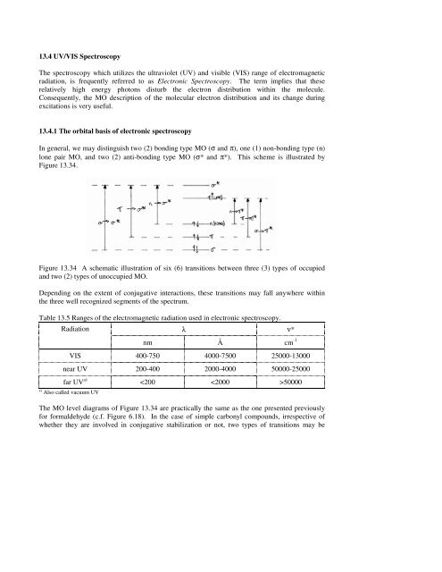
In general, we may distinguish two (2) bonding type MO (σ and π), one (1) non-bonding type (n)
lone pair MO, and two (2) anti-bonding type MO (σ* and π*). This scheme is illustrated by
Figure 13.34.
Figure 13.34 A schematic illustration of six (6) transitions between three (3) types of occupied
and two (2) types of unoccupied MO.
Depending on the extent of conjugative interactions, these transitions may fall anywhere within
the three well recognized segments of the spectrum.
Table 13.5 Ranges of the electromagnetic radiation used in electronic spectroscopy.
Radiation λ ν*
nm Å cm -1
VIS 400-750 4000-7500 25000-13000
near UV 200-400 2000-4000 50000-25000
far UV a)

observed: the low energy (long wavelength) n →π∗ and the higher energy (shorter wavelength)
π→π∗ as illustrated by Figure 13.35.
Figure 13.35 A typical electronic spectrum of a carbonyl compound.
The intensity of the absorption is measured by the molar extinction coefficient (ε) and it is defined
in terms of the incidental (Io) and transmitted (I) light intensity, as well as the concentration of the
solution (c) and the path length (l).
1
ε =
cl
log10
The value of ε may be within a large range of values
when c = 1 mol/L and l = 1cm.
0 ≤ ε ≤ 10 6
I
I
0
[13.34a]
[13.34b]
The greater the ε value, the more probable the absorption. In general, the n→π∗ absorption is
practically “symmetry forbidden” or “overlap forbidden” because the electron is promoted from
the plane of the molecule to a plane which is perpendicular to the molecular plane. This is not the
case for the π→π∗ excitation and therefore, it is an allowed transition, and consequently, more
intense.

Figure 13.36 A schematic illustration of the spatial arrangement of the two lobes of the lone pair n
(which is like a 2py of oxygen) and the four lobes (two + and two -) of the π∗ MO or a carbonyl
functional group.
The wavelength (or wavenumber) depends on the extent of conjugation. This is illustrated by the
data summarized in Table 13.6 and the underlying principle is shown in Figure 13.37.
Table 13.6 Carbonyl transitions as the function of conjugative interaction.
Functional group strong
π→π*
λmax (nm)
weak
n→π*
C=O 166 280
C=C−C=O 240 320
C=C−C=C−C=O 270 350
This change in absorption, due to conjugative interaction, is true not only for carbonyl compounds
but unsaturated hydrocarbons as well (c.f. Table 13.7). Of course in this latter case no n→π∗
transitions are allowed. Only π→π∗ transitions are possible since the molecule contains no lone
pair (n).

Table 13.7 The effect of conjugative interaction on the π→π∗ electronic transitions of unsaturated
hydrocarbons.
π→π*
Functional group λmax (nm) ε
C=C 170 16000
C=C−C=C 220 21000
C=C−C=C−C=C 260 35000
The wavelengths shift towards larger λ values i.e. towards the red (“red-shift”) with conjugative
interaction. Of course, in agreement with [13.1], wavelengths mean smaller wave numbers and
therefore lower excitation energy [13.35]:
ν*
=
λ
1
1
∆E = hcν* = hc
λ
[13.35a]
[13.35b]
An explanation for the above phenomena may conveniently be given in terms of MO levels. This
is illustrated for an unconjugated carbon-carbon double bond in Figure 8.2 and for a nonconjugated
carbonyl in Figure 6.18. The effect of conjugative interaction for C=C−C=C can be
demonstrated in terms of the MO level diagrams of two ethylene molecules (c.f. Figure 13.37).
Figure 13.37 MO level correlation diagram to illustrate the effect of conjugation on the π→π∗
transition of unsaturated hydrocarbons.

Clearly the π→π∗ excitation energy for the conjugated pair of double bonds, ∆E2(π→π∗), is
smaller than the excitation energy for a single, unconjugated double bond, ∆Ε1(π→π∗). The
former one has a longer wavelength absorption in comparison to the latter one.
∆Ε2(π→π∗) < ∆Ε1(π→π∗)
λ (2) max (π→π∗) > λ (1) max (π→π∗)
[13.36a]
[13.36b]
More extensive conjugative interaction exists in the conjugated hexatriene (the last entry in Table
13.7). This can be demonstrated, analogously to that of the situation presented in Figure 13.37, in
terms an MO correlation diagram involving a butadiene (C=C−C=C) and an ethylene (C=C)
molecule.
The effect of conjugative interaction for C=C−C=O can be illustrated in terms of MO level
diagrams for an ethylene and a formaldehyde molecule (c.f. Figure 13.38).
Figure 13.38 MO level correlation diagram to illustrate the effect of conjugation on the n→π∗ and
π→π∗ transition of unsaturated carbonyl compounds.

In the first approximation shown in Figure 13.38, we can assume that the non-bonded (n) lone pair
is not affected by conjugation and, therefore its energy value is unchanged. However, the π and
π∗ levels do change. This influences the transition, promotion or excitation energies, and,
therefore, the wavelength, of both the n→π∗ and the π→π∗ modes of excitation. As a result, we
may recognize the following inequalities:
E2(n→π∗) < E1(n→π∗) [13.37a]
E2(π→π∗) < E1(π→π∗) C = C C = O
≈ E1(π→π∗)
320
[13.37b]
More extensive conjugative interaction, which exists in C=C−C=C−C=O (c.f. last entry in Table
13.6) can be demonstrated, using butadiene and formaldehyde as components.
13.4.2 Spectral shift upon protonation
The various functional groups, which are involved in the determination and/or modification of
electronic spectral characteristics, are frequently referred to as chromophores. The C = C and
C =O functionalities, which previously discussed, are also chromophores. However, there are
other functionalities, which can be regarded as chromophores. Two such groups, which can
exhibit both n→π∗ and π→π∗ excitations, are the imine and the azo groups.
C N N N
imine azo
[13.38]
Whenever lone pair (n)-containing heteroatoms are part of a double-bonded system, they may
undergo protonation under acidic conditions.

(a) (b) (c)
n n
C O C N N N
H (+)
H (+)
C O C N N N
321
H (+)
H H H
(+)
(+) (+)
n
(a) (b) (c)
n
n
[13.39]
[13.40]
As the result of protonation, the lone pair (n) becomes a bonding pair (σ). Furthermore, all
electrons are now held more tightly and so all MO energy levels are lowered. Interestingly
enough, the LUMO is also lowered substantially as shown by Figure 13.39.

Figure 13.39 Spectral red shift of π→π∗ transition upon protonation.
322

What is shown in Figure 13.39 is the basis of a whole class of acid-base indicators, which show a
red shift upon protonation. The two classic examples are Methyl orange (discovered by Griess in
1877) and Methyl red (synthesized by Rupp in 1908). These are amphoteric azo-dyes which are
soluble in both acids and bases [13.41].
O O
Na (+)
(-)
S
O
N N
methylorange
(a)
Me
N
Me
Na (+)
(-)
O C
323
O
N N
methylred
(b)
Me
N
Me
[13.41]
Under acidic conditions, it is not only organic acids liberated from their sodium salts which are
protonated but also one of the two lone pairs of the -N=N- functional group. It appears that the N
on the left hand side is more basic than the N on the right hand side because the NMe2 group
conjugatively stabilizes the protonated azo-dye type indicator, [13.42].
N N
Me
N
Me
Ar Ar
neutral (or alkaline)
solution
(yellow)
+ H (+)
+ H (-)
H
N N
Me (+)
N Me
acidic
solution
(red)
13.4.3 Electron configuration and multiplicities of ground and excited states
[13.42]

It was implied in Figures 13.34, 13.37 and 13.38 that the energy of the VIS or UV radiation is
used for the promotion of an electron when an excitation occurs. Thus, in electronic spectroscopy
we are essentially changing the ground state electronic configuration to one of the excited state
electron configurations. The n→π∗ and π→π∗ excitations of a C=O functionality, are shown in
Figure 13.40.
all
electrons
= =1
S s i
i
324

325
[13.43]
Figure 13.40 Ground and low-lying excited state electron configurations of a carbonyl function
group.
Note that in this figure the spin state is conserved, because in both the electronic ground state and
the electronic excited state, we have the same number of α spins (s=+½) and β spins (s=- ½).
Consequently, the net or overall spin state (S), which is the sum of the individual spins (si), will
add up to zero.
Therefore, we may introduce the concept of multiplicity (m) to characterize the Spin State of the
molecular electron distribution:
m = 2⏐S⏐+1
[13.44]
In the low-lying excited state electron configurations presented in Figure 13.40, the total or overall
spin was zero and therefore, the multiplicity was found to be 1, which is called a singlet:
S = 0 [13.45a]
m = 1 (Singlet) [13.45b]

Practically all organic molecules have singlet multiplicities in their electronic ground state due to
the double occupancy of the MO energy levels. In contrast, free radicals, such as those discussed
in Chapter 9, have half integer spins (i.e. + ½ or -½) and therefore, have doublet multiplicity
([13.46] and Figure 13.41)
S = ±½ [13.46a]
m = 2 | ½ | + 1 = 2 (Dublet) [13.46b]
Figure 13.41 Doublet spin states for an odd number electron-containing chemical system
(e.g. Li).
The two spin states can be described by two wave functions, which yield identical energy values
(double degeneracy) in the absence of a magnetic field. However, their energy values will differ
from each other in the presence of an external magnetic field. This leads to an energy level
diagram (Figure 13.42) is analogous to that in Figure 13.2. However, in the present case, it is
electron spin not nuclear spin, which makes the difference.
326

Figure 13.42 Variation of a free radical electron Spin State (α or β) energy with external magnetic
field (Bo).
This leads to electron spin resonance (ESR) spectroscopy, which will not be discussed further in
these lecture notes.
Returning to the principles of excited configurations generated from closed electronic shell ground
states (characterized by double occupancy) presented in Figure 13.40, we may recognize the
possibility of spin flips. Consequently, we may have two identical spin states (αα or ββ), in
addition to αβ, giving rise to triplet multiplicity [13.47]:
S = Sαα = + ½ + ½ = + 1 [13.47a]
S = Sββ = -½ - ½ = -1 [13.47b]
m = 2 S + 1 = 2 x 1 + 1 = 3 (Triplet) [13.47c]
The electron configuration for the Sαα spin states, associated with the n→π∗ and π→π∗ modes of
excitations, are illustrated in Figure 13.43. Figure 13.43 is an extension of Figure 13.40.
327

Figure 13.43 Singlet and triplet electron configurations of a carbonyl group.
13.4.4 Potential energy curves of ground and excited states
Energy is always a function of molecular geometry, a concept, which we have presented many
times before. Conformational potential energy curves (PEC) and potential energy surfaces (PES)
were covered extensively in Chapters 4 and 5. For stretching potentials, the first example was
seen in Figure 1.7 and the last example was given in this chapter in Figure 13.33.
All of the above were related to the electronic ground states of the molecular systems in question.
It should not be surprising to learn that the same may be applied for electronic excited states.
However, there are some differences that are observed when comparing the details of the excited
PEC or PES with their ground state counterparts. Take for example, a simple carbonyl compound
such as formaldehyde (H2C=O). In the n→π∗ excited state an electron arrives at the antibonding π
orbital, while the electron pair in the bonding π orbital is still present. Due to the third antibonding
π electron, the C=O bond becomes weaker and longer. In the π→π∗ excited
configuration, the situation is somewhat worse because there is only one π electron in the bonding
orbital, while the other π electron is anti-bonding (i.e. π∗). Consequently, the excited state bond
328

lengths will be longer than a genuine C=O double bond but shorter than a σ-type single C−O
bond. In other words, these excited states will have their energy minima somewhere in between
that of H2C=O and H3C−OH. This principle is illustrated schematically in Figure 13.44. The
figure also illustrates the fact that all energy curves have vibrational levels (just like that given in
Figure 13.33) even though only two (the 0 and 1) are specified explicitly in Figure 13.44. Note
that the bottom of the TRIPLET state curve is lower than the bottom of the SINGLET state curve.
This may be regarded as a consequence of the generalized Hund’s rule.
Figure 13.44 Morse type stretching potentials for the low lying electronic states of a typical
carbonyl compound.
329

The spin momentum conservation rule dictates that a transition will occur between the singlet
ground state and one of the singlet excited states. Transition from a singlet to a triplet is
forbidden. However, intersystem crossing from the excited singlet state to the corresponding
excited triplet state De-excitation or relaxation back to the ground state may take place with
simultaneous radiation. When de-excitation originates in the excited Singlet State, it is called
fluorescence (F). When relaxation begins at the excited Triplet State, the process is called
phosphorescence (P). The frequencies of these two modes of de-excitation (i.e. F and P) which
correspond to the energy released, are smaller than the frequency and corresponding energy of the
absorption (A) or excitation [13.48]:
These points are illustrated schematically in Figure 13.45.
νA > νF > νP [13.48a]
∆EA > ∆ΕF > ∆ΕP [13.48b]
λA < λF < λP [13.48c]
Figure 13.45 A schematic illustration of absorption (A) fluorescence (F) and phosphorescence (P)
of a typical organic compound.
The absorption process is more complicated than Figure 13.45 might reveal. Before they are
excited, most ground state molecules occupy their zero point vibrational (ZPV) level. However,
330

the excited molecules may occupy any of the vibrational levels associated with the same
geometry. There are two special cases however,
(i) the vertical (or Frank-Condon) excitation
(ii) the 0 - 0’ (or adiabatic) excitation
(iii)
However, the possibility of the involvement of any vibrational levels in transitions, leads to a
vibrational structure of the absorption spectrum. These principles are illustrated in Figure 13.46.
Figure 13.46 Vertical and adiabatic transitions as well as the vibrational structure associated with
an absorption spectrum (left hand side, side-ways). The IR transition of the ground electronic
state is also marked in at 1700 cm -1 .
In this figure the spectrum is presented side-ways at the left-hand side. The vertical (or Frank-
Condon) transition is usually the most intense vibrational peak corresponding to λmax (c.f. Figure
13.35). The weakest low energy section (i.e. the tail end in Figure 13.35) is where the 0 - 0’ (or
adiabatic) transition is located. When no vibrational structure is found, the maximum (i.e. λmax)
still corresponds to the vertical transition.
One of the most ordinary compounds with a vibrational structure in its UV absorption
spectrum is benzene (c.f. Figure 13.47).
331

Figure 13.47 UV spectrum of benzene showing the molecular vibrational structure.
Carbonyl compounds do not often show vibrational structure. However, under certain
circumstances, with appropriate substitution for X in X−C=O, the n→π∗ transitions have sharp
vibrational structures. In this case, the vibrational spacing is much less than 1600 or 1700cm -1 ,
which is the typical ground state C=O stretch and a little bit larger than the characteristic
frequency of the C−O stretch (1000 - 1100cm -1 ). Thus, the spacing between the vibrational peaks
corresponds to the vibrational levels of the particular excited state and in this state the CO bond is
located somewhere in between a single and a double bond (c.f. Figure 13.48).
332

Figure 13.48 Carbonyl n→π∗ transitions for selected compounds of the type Ph3X−CO−Ph
The upper left hand side of Figure 13.48 shows that the heavy atom substitution (i.e. C → Si or C
→ Ge)
(i) shifts the absorption frequency (ν∗) towards the visible (red-shift) and the compounds
become colored (note: 25,000cm -1 = 400nm)
(ii) accentuates the vibrational structure which was hardly noticeable in Ph3COPh
The lower left hand side of Figure 13.48 shows that the observed envelope curves, for X = Si and
Ge, of the spectra, showing partially resolved vibrational fine structures, may be deconvoluted to
Gaussian components. These Gaussian components are representing the transitions to individual
vibrational levels of the n→π∗ excited states. The characteristic values of these vibrational bands
are summarized in Table 13.8.
The right hand side of Figure 13.48 provides an explanation of the red shift in terms of d-orbital
participation of the heavy atom (X = Si, Ge). Combining for example, the C=O with Si to
produce a Si−C=O system, leads to a small increase in all three C=O levels because the inductive
effect of Si is followed by a splitting of the π - levels as they interact with a vacant d-orbital on Si.
Table 13.8 Results of resolution of n →π∗ bands of triphenylsilyl phenyl and triphenylgermyl
phenyl ketones into gaussian components
333

Assigned
transition
Peak position
ν*
(cm -1 )
334
Molar extinction
coefficient
Triphenylsilyl phenyl ketone
0→0 1 22.350 168
Vibrational spacing
∆ν*
(cm -1 )
0→1 1 23.540 285 1190 a)
0→2 1 24.00 195 1160
0→3 1 25.740 106 1040
0→4 1 26.730 35 990
Triphenylgermyl phenyl ketone
0→0 1 22.660 133
0→1 1 23.880 246 1220 a)
0→2 1 25.080 180 1000
0→3 1 26.210 100 1130
0→4 1 27.260 40 1050
a) Fundamental vibrational frequency of the n→π* electronic excited state
13.4.5 Cis-trans isomerization and photochemistry
The potential energy curve for a thermal cis-trans isomerization was presented earlier (c.f. Figure
8.1). Photochemical isomerization also involves excited state conformational potential energy
curves as well. In most cases the excited state potential energy curves are in different phases with
respect to the ground state. This is due to the fact that the minimum energy conformers of the
excited states are different from that of the ground state. In the case of an olefinic double bond the
excited state conformation is not planar but twisted out of plane by 90°.

Figure 13.49 Twisted geometry of singlet and triplet excited ethylene.
The schematic potential energy curves for the ground and excited states of 1,2-disubstituted
ethylene are shown in Figure 13.50.
335

Figure 13.50 A schematic illustration of a photochemical cis-trans isomerization.
The photochemistry of vision is related to cis-trans isomerization. A molecule called rhodopsin,
which is made up of 11-cis-retinal and a protein called opsin, undergoes cis-trans isomerization
upon radiation with visible light [13.49].
336

Me
Me
Me
Me
Me
Me
Me
11 12
Me C
hν
Me
13
Me
337
(11 - cis)
N
(all trans)
Protein
Me Protein
During the past half a century, a great deal has been discovered about photochemical reactions.
Clearly, in addition to vision, photochemistry is of great importance in nature because
photosynthesis in plants is based on the harnessing of the energy of sunlight. As it turns out,
laboratory experiments have demonstrated that one can achieve many reactions photochemically,
which do not proceed thermally. However important these photochemical reactions may be, they
will not be discussed in these lecture notes at this time.