PhD. thesis - Univerzita Karlova

Institute of Petrology and Structural Geology 

Faculty of Science 

Charles University 

Prague, Czech Republic 

NUMERICAL APPROACHES IN 

STRUCTURAL AND 

MICROSTRUCTURAL ANALYSES 

Ph.D. thesis by 

ONDREJ LEXA 

Mgr., Comenius University 

in Bratislava, 1995 

Supervised by 

Prof. RNDr. Karel Schulmann, CSc. 

A thesis submitted to the 

Faculty of Science, Charles University 

of the requirements for the degree of 

Doctor of Philosophy 

Institute of Petrology and Structural Geology 

2003 

Jury Prague, 2003 

Prof. RNDr. František HROUDA, CSc. (Charles Univ., Prague) Head of the Jury 

Prof. Jean-Pierre BURG (ETH, Zürich) Reviewer 

Prof. Jean-Marc LARDEAUX (ETH, Zürich) Reviewer 

Dr. John Cosgrove (Imperial College, London) Member of the Jury 

Doc. RNDr. Ondřej Čadek, CSc. (Charles Univ., Prague) Member of the Jury 

Doc. RNDr. Dušan Plašienka, CSc. (Acad. of Science, Bratislava) Member of the Jury

Acknowledgements 

Al though a PhD the sis is of fi cially a work of one per son, it stems from dis cus sions, 

ex changes of ideas and ex pe ri ences col lected dur ing the course of a the sis. I would like to 

thank the In sti tute of Pe trol ogy and Struc tural Ge ol ogy for pro vid ing a stim u lat ing en vi ron ment, 

re sources and fund ing for my re search assistantship through out this PhD. 

There are many peo ple to thank for their sup port and en cour age ment, without whom 

this thesis would have been impossible, improbable, and/or impoverished. 

Firstly spe cial thanks to my su per vi sor, Prof. Karel Schulmann, whose en thu si as tic cry 

of ‘Any Prog ress’ will haunt me for the rest of my days - his un quench able cu ri os ity and love for 

the sub ject are prob a bly the most valu able les sons I have learned from this PhD, and his 

con tin uous sup port and en cour age ment have kept me go ing over the last six or so years. 

Thanks also to the many col leagues I’ve worked with, par tic u larly Pavla, Lenka, 

Zdeněk, Kony, Stano, Láďa and oth ers - whose sug ges tions and/or guid ance were al ways 

much ap pre ci ated. 

Next there are all the friends I’ve made, the list is too long to men tion but their 

friend ship, drink ing or sing ing skills helped to make my stay in Prague a re ally happy one. 

Much ap pre ci a tion goes to my Mom and Dad and the rest of my fam ily, who have been 

great over the years and never raised an eye brow when I claimed my the sis would be fin ished 

in the “next two weeks” for cou ple of years… 

Last, but cer tainly not least, I thank my girl friend, Markéta, whose love gave me the 

strength and en cour age ment to fol low the path that I felt was right, and whose pa tience al lowed 

me the free dom to com plete the task. This PhD. is lov ingly ded i cated to her. 

A big, big THANK YOU to all of you.

Publications: 

Lexa, O. and Bezák, V. (1996): Porphyric granitoids in the western part of the Slovenske 

rudohorie Mts.: Emplacement and deformation in shear zones. Slov. Geol. Mag., 3-4, 

D.Štúr Publ., Bratislava, 189-197. 

Madarás, J., Hók, J., Siman, P., Bezák, V., Ledru, P., Lexa, O. (1996): Extension tectonics and 

exhumation of crystalline basement of the Veporicum unit (Central Western 

Carpathians). Slov. Geol. Mag., 3-4, D.Štúr Publ., Bratislava, 179-183. 

Lexa, O. and Schulmann, K. (1999): Cretaceous evolution of the Variscan basement of the SE 

Western Carpathians: Combination of continental underthrusting and indentation 

tectonics, Geologica Carpathica, 50, 119-120. (Extended abstract) 

Nemčok, M., Konečný, P., Lexa, O. (2000): Calculations of tectonic, magmatic and residual 

stress in the Štiavnica stratovolcano, Western Carpathians: Implications for mineral 

precipitation paths, Geologica Carpathica, 51, 1, 19-36. 

Konopásek, J., Schulmann, K., Lexa, O. (2001): Structural evolution of the central part of the 

Krusne hory (Erzgebirge) Mountains in the Czech Republic - evidence for changing 

stress regime during Variscan compression. Journal of Structural Geology, 23(9): 

1373-1392. 

Schulmann, K., A. B. Thompson, O. Lexa, and J. Ježek ( 2003): Strain distribution and fabric 

development modeled in active and ancient transpressive zones, J. Geophys. Res., 

108(B1), 2023 

Konopásek, J., Schulmann, K., Lexa, O. 2003. Reply to comments by A. Krohe and A.P. 

Willner on “Structural evolution of the central part of the Krusne Hory (Erzgebirge) 

Mountains in the Czech Republic—evidence for changing stress regime during 

Variscan compression”: [Journal of Structural Geology 23 (2001) 1373-1392]. Journal 

of Structural Geology 25(6), 1005-1007. 

Lexa, O., Schulmann, K., Ježek, J. (2003): Cretaceous collision and indentation in the West 

Carpathians: view based on structural analysis and numerical modeling, Tectonics, 

accepted. 

Lexa, O., Cosgrove, J., Schulmann, K. (2003): Apparent shear-band geometry resulting from 

oblique fold sections, Journal of Structural Geology, accepted. 

Abstracts and presentation: 

Madarás, J., Hók, J., Kováč, P., Lexa, O. (1995): Cretaceous extensional tectonics in the 

junction area between Veporicum and Gemericum units, West Carpathians, Slovakia., 

Terra Abstracts, Abstract suppl. No.1, vol. 7, s. 123. 

Onačila ,D., Nemčok, M., Lexa, O., Lexa, J. (1995): Structural factors of ore deposition: 

Banská Štiavnica mining district., Terra Abstracts. Abstract suppl. No. 1, vol. 7, s. 292.

and deformation of lithospheric structure described above. A numerical approach that enables 

us to model the deformation in a weak zone (Gemer Unit) surrounded by a rigid (Vepor Unit) or 

free boundaries is presented here. This approach is based on the thin viscous sheet 

approximation for modeling of the deformation. The Gemer Unit is assumed to be a horizontal 

weak tabular domain subjected to flow with no tractions at top and bottom surfaces. We also 

assume that vertical gradients of the horizontal velocity are negligible, which allows us to 

integrate the equations of motion over the vertical dimension and to work with vertical averages 

of stress and strain rate. The details are presented in appendix of Chapter 1. Using the 

assumption of Newtonian behaviour (linear relation between stress and strain rate), the 

procedure leads to a system of elliptic partial differential equations for two horizontal velocity 

components. The system is solved by the finite element method with boundary conditions, 

which represent the geological situation. In each time increment, boundaries are rearranged 

simultaneously with repeating solution of the governing equations for the velocity. At each time 

step we evaluate instantaneous strain rate and finite strain in a net of points in the domain. These 

numerical exercises significantly contribute to understanding of reasons of local changes in 

deformational regime due to deformation and help us to explain the origin of major structural 

features in studied area. 

During field studies in the West Carpathians we encountered a considerable problem 

related to Cretaceous extensional tectonics affecting the Vepor crystalline 

basement. The previous studies have resulted in the generally accepted model of post-orogenic 

or orogen-parallel extension. These studies are supported by geochronology, petrology, and 

particularly by interpretations of kinematic indicators namely, shear-bands. Our field revision 

points out that extensional tectonics was in fact the first Alpine deformation in the studied area 

and that it pre-dates the compressional stage of Alpine tectonic evolution. This causes that in 

many cases we deal with oblique sections across small-scale folds or crenulation cleavage, 

which are likely to be misinterpreted as shear-bands. In Chapter 2 we demonstrate that: 

1) distinguishing between compressional and extensional crenulation cleavages is not always 

an easy task, 2) unless this is fully appreciated there is a great danger of misinterpretation when 

the shear bands are used as kinematic indicators, 3) the compressional and extensional 

crenulation cleavages can appear identical when seen on flat outcrop surfaces or in thin 

sections. This work aims to alert that because the shear bands are such noticeable structures and 

their kinematic significance is straightforward, without detailed knowledge of 3D geometry of

structure, compressional crenulation cleavage could be misinterpreted as shear bands and 

consequently, erroneous structural and kinematic interpretation could be proposed. 

The structural study of the Gemer-Vepor system of the West Carpathians has shown 

that the collisional systems have to be regarded as a result of continuous structural 

evolution in which the polyphase deformational pattern results from instabilities, which are 

active in different time at different places of the system. The complex boundary conditions may 

allow us predict the development of mechanical instabilities as a function of size of indenter and 

location of rigid blocks. Being aware of close link between applied boundary conditions and 

unique deformational pattern developed in some way, we attempted to solve an inverse 

problem. The aim was to find an explicit relation between internal parameters (i.e. measurable 

features like finite strain intensity, orientation of planar and linear fabric) and external 

parameters (characteristics, which are usually not directly measurable like strain rate, duration 

of deformation, velocity field, elevation of rock samples etc.). Results of this approach used in 

a study of strain distribution and fabric development in transpressional regime with free slip 

boundaries are presented in Chapter 3. We showed that the strain symmetry is sensitive to the 

angle of convergence, whereas the strain intensity parameter D is well correlated with 

across-width shortening of a transpressional zone. We produce "strain map" where a unique set 

of internal parameters corresponds to a unique set of external parameters, i.e. in a simple case, 

the angle of convergence, strain rate for given duration and sample elevation could be depicted 

from strain parameters K and D. We immediately recognized disparity between calculated and 

naturally measured values. To make these considerations more realistic, a concept of 

deformation partitioning was therefore introduced. We examined in detail three major styles of 

deformation partitioning and we showed that (1) discrete partitioning results in general decrease 

in finite strain accumulations and in increase in pure shear component, (2) ductile partitioning 

splits the transpressional domain into a pure shear zone where strain accumulation decreases 

and in a wrench-dominated zone where strain accumulation increases, and (3) viscosity 

partitioning is marked by difference in strain rates in zones of different viscosity and therefore 

results in more rapid elevation in the low viscosity domain. Furthermore the possibility of 

lineation switch for low angle transpression is reached much earlier. We also showed that any 

type of deformation partitioning results in decrease in average finite strain intensity causing 

enhancement of pure shear component in the system. This may explain why generally small 

finite strains are measured in nature and why many orogenic belts are considered to be a result 

of frontal convergence.

2.1. Pre-Cretaceous geology of the studied area 

The studied area is located in the southern part of the CWC and comprises three major 

lithological and tectonometamorphic units (Fig. 1). From the north to the south and from the 

bottom to the top they are 1) Variscan crystalline basement (Vepor Unit) with Late Paleozoic 

and Mesozoic cover sequences, 2) Early to Late Paleozoic, basinal, mostly low grade turbiditic 

sequences (Gemer Unit), and 3) Mesozoic accretionary wedge containing blueschist facies 

relics overlain by 4) flat non-metamorphosed Silica nappe. 

2.1.1. Variscan crystalline basement - the Vepor Unit. The crustal rocks of the Vepor 

basement are composed of two contrasting Variscan metamorphic domains exhibiting 

pre-Alpine thrust tectonics. Structurally lower domain, generally dipping to the north, is 

composed of medium-grade schists exhibiting peak PT conditions in Ky-St micaschists 

corresponding to max. 10 kbars and 550°-600°C [Korikovskij et al., 1989; Méres and Hovorka, 

1991]. The classic Barrow type metamorphic zonation is difficult to establish due to the Alpine 

greenschist facies overprint but in the eastern part of the Vepor basement (Čierna Hora Mts), 

a metamorphic zonation ranging from biotite zone in the south to staurolite zone in the north is 

documented [Jacko et al., 1990; Korikovskij et al., 1990]. Structurally higher crystalline unit is 

represented by a domain of heterogeneous para- and ortho-derived migmatites intruded by 

porphyritic to medium-grained peraluminous granites. The Variscan age of metamorphism is 

docummented by Th-U-Pb dating of monazite [370-350 Ma, Janák et al., 2001a] and by 

sporadically preserved 40 Ar/ 39 Ar cooling ages ranging from 358 to 312 Ma [Dallmeyer et al., 

1996]. High-grade fabrics represented by compositional layering and stromatitic banding in 

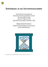
migmatites are dipping either to the NW or to the N under steep to medium angles. Peak 

temperature conditions yield 680 - 730°C at pressures of 4 - 6 kbars (Fig. 2) [Siman et al., 1996]. 

These PT conditions most likely correspond to late exhumation and decompression melting. 

This is deduced from other parts of West Carpathians where relics of high-pressure assemblages 

preserved in similar types of migmatites were found [Hovorka and Méres, 1989; Janák et al., 

1996]. 

The southern Vepor Variscan crystalline basement is unconformably covered by Late 

Carboniferous (Stephanian) sandstones and shales [Planderová and Vozárová, 1978]. These 

metasediments were intruded by granitoids that were responsible for contact metamorphism 

ranging from biotite to cordierite zones. Contact metamorphic conditions of 500°C and 2 kbars 

were established by Vozárová [1990]. This author also suggests that contact metamorphism 

overprinted regional greenschist facies assemblages of Carboniferous metasediments. The 

16

Unit is regarded as a relic of the Variscan internal domain in which the anatectic lower crust is 

thrust over the middle crustal Barrovian complex. The original Paleozoic relationship between 

Vepor and Gemer Units is largely obscured by later Mesozoic evolution. North dipping 

pre-Mesozoic fabrics and increase in metamorphic grade from the south to the north in both the 

Gemer and Vepor Units suggest an existence of N-S polarity of Paleozoic orogeny [Bezák, 

1992; Faryad, 1990]. Based on these data, the Klátov and Rakovec groups may be interpreted as 

relics of Early Paleozoic basin underthrust beneath the high-grade rocks of the internal domain 

represented by the Vepor Unit to the north. In our model the whole nappe stack was further 

thrust over Early Paleozoic basin represented by the Gelnica Group, which is probably 

underlain by a Neo-Proterozoic basement (Fig. 2). The lack of thrust-related structures in 

Middle Carboniferous metasediments indicates that the nappe stacking occurred in 

pre-Westfalian times. 

The southward thrusting of high-grade gneisses over the low-grade mostly 

metasedimentary foreland formed two promontories separated by embayment of weakly 

metamorphosed sediments. This irregular geometric distribution of gneissic complexes and soft 

sediments played critical role in the subsequent Mesozoic tectonic evolution. 

The last major pre-Cretaceous tectonic event responsible for the final structural pattern 

was the Jurassic southeastward subduction (in recent coordinates) of the Meliata ocean and the 

southern passive margin of the European platform. This process resulted in formation of an 

accretionary wedge and its northwestward obduction over both the Gemer and Vepor Units 

during the Late Jurassic [150 - 160 Ma, Dallmeyer et al., 1996; Faryad and Henjes-Kunst, 1997; 

Maluski et al., 1993] (Fig. 2). In the southern part of the Gemer Unit, sedimentary bedding is 

well preserved and folded by large-scale open folds with N-S trending hinges (Fig. 3). This 

folding is connected with development of spaced cleavage steeply dipping to the east 

suggesting that thethinned continental margin was intensively reworked during Jurassic 

subduction processes. 

3. Cretaceous polyphase structural evolution - collisional stage 

Cretaceous collisional evolution of the Gemer and Vepor Units is marked by four major 

distinct tectonic events: 1) Formation of the Gemer Cleavage Fan (GCF) structure affecting 

central part of the Gemer Unit, 2) extensional deformation of the western Vepor promontory, 

3) transpressional shearing affecting the western Vepor promontory and development of the 

Trans-Gemer Shear Zone (TGSZ), 4) extrusion of the Gemer Unit over the eastern Vepor 

promontory along the Eastern Gemer Thrust (EGT). 

19

3.3. Cretaceous transpressional deformation - Trans-Gemer Shear Zone 

(TGSZ) 

The transpressional deformation is marked by development of a several kilometer wide 

zone of NE-SW trending steep cleavage along the southern boundary of the western Vepor 

promontory (Fig. 5b). Here, in the Gemer Unit, Carboniferous and Permian cover of the Vepor 

basement and Mesozoic rocks of the Meliata accretionary wedge, all previously developed 

structures, are intensively reworked under lower greenschist facies conditions. In the strongly 

attenuated Gemer Unit, relics of E-W trending GCF fabric and new NE-SW trending cleavage 

form a map-scale sigmoidal domain surrounded by highly sheared Late Paleozoic rocks 

(Fig. 5b). Locally, the early-developed foliation is refolded by synschistose noncylindrical 

folds with steeply to subhorizontally plunging hinges, which become subparallel to horizontall 

stretching lineations with increasing finite strain (Fig. 4d). These features are consistent with 

progressive folding in transpressional shear zones [Fossen and Tikoff, 1998; Treagus and 

Treagus, 1992]. 

The boundary of the Vepor basement and Late Paleozoic cover is intruded by sheets of 

peraluminous granites, which show magmatic fabric parallel to the transpressional shear zone. 

In some places, heterogeneous, steep NE-SW trending mylonitic S-C fabric indicates sinistral 

shearing. Granite apophyses and dikes are folded and sheared or they crosscut the foliation of 

host rocks without internal deformation. All these features are consistent with syntectonic 

character of granite emplacement. Shallow level of magma emplacement is documented by 

contact metamorphism of host Late Paleozoic schists [500°C and 2 kbars, Vozárová, 1990]. 

Towards the NE, this 5 km wide zone of steep cleavage continues into central part of the 

Gemer Unit (Figs. 3a, 4e). This NE-SW trending zone of shear deformation - the Trans-Gemer 

Shear Zone (TGSZ) overprints all previously developed metamorphic fabrics exhibiting a 20 to 

25 km sinistral offset of lithological stripes and axial zone of GCF. The displacement and 

intensity of deformation gradually vanishes towards the NE edge of the Gemer Unit. 

Two several kilometers wide NE-SW trending zones of greenschist facies 

transpressional deformation affected internal parts of the Western Vepor promontory (Fig. 5b). 

Inside these shear zones, the Variscan as well as Mesozoic mylonitic extensional fabric are 

strongly refolded and transposed. The character of folding as well as numerous sense of shear 

criteria underline the sinistral sense of movement. These zones are preferentially developed in 

weak lithologies such as garnetiferous micaschists or highly anisotropic extensional mylonites. 

Outside of these shear zones, weak E-W trending crenulation cleavage affects flat Cretaceous 

extensional mylonitic foliation. The structural mapping shows anticlockwise rotation of this 

25

characterized by north vergent collision of southern continent with northerly lying West 

Carpathian domain (European plate). Fragments of the southern continental domain, now 

located in northern Hungary (Bükk mountains), are considered to be Neo-Proterozoic in age as 

documented by Rb-Sr dating [Pantó et al., 1967]. Here, the absence of Variscan overprint is 

manifested by continuous sedimentation from the Early to Late Paleozoic. We suggest that this 

southern continent behaved as a rigid indenter controlling the deformation of all northerly 

foreland crustal units, and in our coordinate system was actively moving towards the north. The 

mechanical contrast between the Vepor basement promontories and the Gemer slates results 

from their contrasting lithologies and pre-Cretaceous evolution. The interval of thermal 

relaxation of the Vepor quartzofeldspathic crust between the last (Late Carboniferous) 

important thermal perturbation and Cretaceous collision corresponds to about 180 Ma. This 

indicates, that the geotherm of the Vepor crust was equilibrated at the onset of Cretaceous 

orogeny [Cloetingh and Burov, 1996; Morgan and Ramberg, 1987]. Therefore, we suggest that 

the Variscan Vepor basement, composed of gneisses and granites, represented a mechanically 

strong promontory of irregular shape. In contrast, the Gemer Unit is represented mainly by 

low-grade slates composed of fine-grained hydrous minerals with rheology controlled by 

diffusion type of deformation mechanisms as pressure solution and diffusive mass transfer 

[Knipe, 1979; Knipe, 1989]. For the same geotherm, as compared with laterally adjacent 

quartzofeldspathic rocks, the strength of Gemer slates was incomparably lower. Taking into 

account these rheological assumptions, the Gemer Unit during the Cretaceous event is 

considered to be the weakest domain accommodating most of the viscous deformation. 

In agreement with Woodcock et al., [1988] and Sintubin [1999], the cleavage patterns in 

deformable weak rocks reflect the geometry and direction of movement of rigid blocks. In order 

to model the development of superposed cleavage pattern described above, it is important to 

define boundary conditions. 

4.1. Definition of kinematic frame 

The asymmetry of the GCF can be interpreted as a result of movement of rigid indenting 

block to the north and back thrusting of metasediments over its northern margin. The rigid 

basement does not crop out, but it can be traced in deep seismic lines 2T and G1 [Tomek, 1993; 

Vozár and Šantavý, 1999; Vozár et al., 1996]. The seismic profiling shows that the Gemer Unit 

is about 5 km thick sheet-like body resting on a basement of unknown age. This major 

lithological boundary is represented by series of strong horizontal reflectors. The most 

spectacular structure in seismic line G1 [Vozár and Šantavý, 1999; Vozár et al., 1996] is 

27

a highly reflective south-dipping zone along which the horizontal base of the Gemer Unit is 

displaced to the north. This zone is interpreted as the major Sub-Gemer thrust fault responsible 

for northward thrusting of rigid basement over weak sediments resulting in the development of 

GCF (Fig. 6). 

Important question in our model is the displacement of Vepor basement rocks with 

respect to the Gemer Unit. It is well-known that the whole central and southern Carpathian 

domain was actively moving to the north (in recent coordinates) as documented by Cretaceous 

progressive closure of Mesozoic Fatric basinal domain north of the Vepor basement [Plašienka, 

1997]. In this kinematic frame all units are shifted to the north but only differential movements 

within the Vepor-Gemer system are responsible for its internal deformation. Important 

observation is that the deformation intensity in central part of the Gemer Unit vanishes to the 

north. In this area, the Vepor basement is present (covered by Tertiary sediments) but no 

increase in Cretaceous deformation intensity has been observed. This means that this Vepor 

segment does not creating important deformation resulting from possible movement to the 

south. Therefore, we suggest that the Vepor promontories did not move actively to the south, 

and extreme deformation along western and eastern Vepor promontories was imposed by 

generally northward flow of weak material. In conclusion, the only differentially moving rigid 

block is northward thrusted part of sub-Gemer basement. All other basement units can be 

further considered kinematically fixed. 

Our field studies showed that apart from GCF, an intense deformation was concentrated 

along southeastern edge of the western Vepor promontory producing TGSZ and also along 

southwestern edge of the eastern Vepor promontory responsible for the origin of EGT (Fig. 6b). 

The development of TGSZ probably results from a major change in mutual translation direction 

of southern sub-Gemer block and western Vepor promontory due to their oblique collision at 

deeper crustal levels. Localized transpressional deformation in upper crustal levels is a typical 

expression of oblique convergence in many active regions, e.g., San Andreas fault zone 

[Teyssier and Tikoff, 1997], Sumatra [Tikoff and Teyssier, 1994] or Alpine fault in New 

Zealand [Teyssier et al., 1995]. 

4.2. Numerical modeling of progressive deformation of the Gemer Unit 

The presented numerical approach enables to model the deformation in a weak zone 

surrounded by rigid blocks or free boundaries. The approach is based on the thin viscous sheet 

approximationbeing similar to that one used by England et al. [1985] for modeling the 

deformation of the whole lithosphere. We assume horizontal weak tabular domain to have been 

28

Figure 7: a) Initial geometry and boundary conditions of the numerical model. The arrow indicates the velocity 

and trajectory of the indenter northern margin. v=0 – zero Dirichlet boundary condition for velocity, Outflow – 

zero Neumann boundary condition for velocity, b) Finite strain pattern developed in weak zone after 1 Ma of 

shortening. Distribution of strain intensity expressed in D value and orientation pattern of XY plane of finite strain 

ellipsoid. The foliations trajectories are shown by lines and the orientation of lineation is expressed by the color of 

foliation trace. White line corresponds to horizontal lineation and black line to vertical one. c) Finite strain pattern 

developed in weak zone after 3 Ma of shortening. Distribution of strain intensity expressed in D value and 

orientation pattern of XY plane of finite strain ellipsoid, d) Distribution of finite strain symmetry expressed in K 

value. c) Orientation pattern of XY planes and X axes of finite strain ellipsoid. 

subjected to flow with no tractions at top and bottom surface. We consider vertical gradients of 

the horizontal velocity to be negligible, which allows us to integrate the equations of motion 

over the vertical dimension and to work with vertical averages of stress and strain rates. When 

linear constitutive relation between stress and strain rates is considered, the procedure leads to 

a system of elliptic partial differential equations for two horizontal velocity components (see 

Appendix). The system is solved by the finite element method, with the Dirichlet and Neumann 

boundary conditions applied to segments of the domain boundaries corresponding to the 

described geological settings (rigid indenter, free inflow or outflow of material). The vertical 

strain rate and velocity are related to the horizontal velocity field by the incompressibility 

equation. It has been described by Ježek et al. [2002] that the thin sheet model is sensitive to the 

angle of collision and may produce a zone dominated by lateral simple shear close to the 

29

However, the presented model has serious limitations. We are not able to simulate the 

deformation of those parts of the viscous sheet, which were thrust over rigid promontories. This 

particularly concerns extensional stripping of the Gemer Unit from northeastern part of the 

western Vepor promontory. The non-coaxial extensional deformation in this area is most likely 

related to the activity of TGSZ and corresponds to pulling the allochtonous Gemer Unit 

associated with sinistral shearing along this major shear zone. The model is unable to 

demonstrate the effects of strain localization associated with discrete partitioning. In fact, the 

TGSZ is passively translating southern part of the Gemer Unit without significant internal 

deformation. Similarly, the development of EGT appears to be a more localized feature than is 

shown in our model, and leads also to passive thrusting of the Gemer Unit over the eastern 

Vepor promontory. 

Despite of these limitations, the presented model allows to predict the strain pattern in 

front of indenting plate in an area with complex boundary conditions. Our model is intended to 

quantify the cleavage patterns developed due to the movement of rigid blocks as suggested by 

Woodcock [1988], Sintubin [1999] and others. The basis of our modeling is the assumption that 

the cleavage represents the XY plane of finite strain ellipsoid [Cloos, 1947; Sorby, 1853; Wood, 

1974]. Our model works with deformation of originally isotropic medium and does not take into 

account problems of existing internal anisotropy [Cobbold et al., 1971]. However, the major 

advantage of our approach is the interconnection of complex kinematic frame with finite strain 

pattern, which was so far possible only for extremely simple boundary condition models, e.g., 

simple shear, transpression, etc. In addition, the model allows to explain the polyphase cleavage 

patterns in terms of the complex shape of promontories and changes in movements of indenting 

blocks. Moreover, using the regional mapping of cleavage patterns we are now able to 

distinguish actively moving blocks from stationary rigid promontories. 

We are aware that infinite numbers of boundary conditions exist, which may generate 

different strain distribution and superposition of structures. Therefore, we deliberately selected 

the set of boundary conditions, which satisfy the structural evolution in the weak domain 

represented by the Gemer Unit. Such a type of modeling could be used to validate chosen 

boundary conditions, i.e., the role of rigid promontories for complex structural evolutions in 

terrains with polyphase deformation. 

5.2. Time scales of the proposed model 

The time scale of the model is controlled by velocity of the indenting block. We have 

chosen the arbitrary velocity of 1cm/y for the sake of simplicity. However, in the case of Vepor 

33

and Gemer Units, we can define the velocity of movement of our kinematically fixed system. 

Based on the knowledge of approximate initial width and stratigraphic record of the Mesozoic 

(Fatric) basin in front of the Vepor basement [Plašienka, 1997], the rate of shortening is 

estimated to be about 1cm/y, and the duration of the shortening process is estimated at about 

20 Ma. Plašienka [1997] also demonstrated that the original frontal closure of the Fatric Basin 

passed to transpressive movements after 20 Ma. This means that the differential movement of 

rigid indenter, which moves together with the whole kinematic system, has to generate a defined 

finite strain at the same period of time. Moreover, the initiation of TGSZ activity may 

correspond to a transition from frontal to transpressional movements recorded in the northern 

edge of the whole kinematic system. Once this rough time scale is established, then the absolute 

velocity of our indenter should be four times slower than suggested in the model to generate the 

observed strain pattern. 

5.3. Development of topography, exhumation and asymmetry of GCF 

The model allows to estimate average vertical strains, and because of a fixed lower 

boundary condition, also the vertical elevation. We can expect that the surface elevation 

represent local topography generated by shortening of the viscous sheet. The lateral distribution 

of topography follows the exponential distribution of finite strain in areas of pure 

shear-dominated deformation. Fig. 12 shows the distribution of topography in front of an 

indenting block after 7 Ma of shortening. It is to be noted that the domain of highest topography 

follows the axial zone of the GCF, where the degree of metamorphism associated with the 

development of cleavage is most important. 

Although our model predicts vertical cleavage in the entire domain, we observe that the 

cleavage forms a positive fan-like structure. We interpret this pattern as a result of different 

amount of vertical shortening due to different gravitational potential across the GCF. This 

mechanism is manifested by the development of late kink bands with kink planes perpendicular 

or oblique to strongly developed vertical cleavage. 

Acknowledgements. We are grateful to the Geological Survey of the Slovak Republic for 

significant financial support during the initial stages of our research. This work has been also 

supported by the Grant of Charles University Agency No. 216/1999/B-GEO. The salaries of K. 

Schulmann and O. Lexa were covered from the grant of the Ministry of Education 

No. 24313005. 

34

Faryad, S.W., and F. Henjes-Kunst, Petrological and K-Ar and Ar-40-Ar-39 age constraints for the 

tectonothermal evolution of the high-pressure Meliata unit, Western Carpathians (Slovakia), 

Tectonophysics, 280, 141-156, 1997. 

Finger, F., and I. Broska, The Gemeric S-type granites in southeastern Slovakia: Late Palaeozoic or 

Alpine intrusions? Evidence from electron-microprobe dating of monazite, Schweiz. Mineral. 

Petrogr. Mitt., 79, 439-443, 1999. 

Fossen, H., and B. Tikoff, Extended models of transpression and transtension, and application to 

tectonic setting, in Continental transpressional and transtensional tectonics., vol. 135, 

Geological Society Special Publications, edited by R.E. Holdsworth, R.A. Strachan and J.F. 

Dewey, pp. 15-33, Geological Society of London, London, United Kingdom, 1998. 

Genser, J., J.D. Van Wees, S. Cloetingh, and F. Neubauer, Eastern Alpine tectono-metamorphic 

evolution; constraints from two-dimensional P-T-t modeling, Tectonics, 15, 584-604, 1996. 

Hók, J., P. Kováč, and M. Rakús, Structural investigations of the Inner Carpathians - results and 

interpretation, Miner. Slovaca, 27, 231-235, 1995. 

Hovorka, D., and S. Méres, Relicts of high-temperature metamorphic rocks in the Tatro-Veporicum 

crystalline of the Western Carpathians (in Slovak), Miner.Slovaca, 21, 193-201, 1989. 

Jacko, S., S.P. Korikovskij, and V.A. Boronichin, Equilibrium assemblages of gneisses and 

amphibolites of Bujanová complex (Čierna Hora), Eastern Slovakia, Miner.Slovaca, 22, 

231-239, 1990. 

Janák, M., M. Cosca, F. Finger, D. Plašienka, B. Koroknai, B. Lupták, and P. Horváth, Alpine 

(Cretaceous) metamorphism in the Western Carpathians: P-T-t paths and exhumation of the 

Veporic core complex, Geol. Paläont. Mitt. Innsbruck, 25, 115-118, 2001a. 

Janák, M., P.J. O'Brien, V. Hurai, and C. Reutel, Metamorphic evolution and fluid composition of 

garnet-clinopyroxene amphibolites from the Tatra Mountains, Western Carpathians, Lithos, 39, 

57-79, 1996. 

Janák, M., D. Plašienka, M. Frey, M. Cosca, S.T. Schmidt, B. Lupták, and S. Méres, Cretaceous 

evolution of a metamorphic core complex, the Veporic unit, Western Carpathians (Slovakia): 

P-T conditions and in situ Ar-40/Ar-39 UV laser probe dating of metapelites, Journal of 

Metamorphic Geology, 19, 197-216, 2001b. 

Ježek, J., K. Schulmann, and A.B. Thompson, Strain partitioning, strike slip faulting and the 

development of strain parameters in front of an obpliquely convergent indenter, in Continental 

collision and Tectonosedimentary evolution of forelands, EGS Special Publication Series, 

edited by G. Bertotti, K. Schulmann and S. Cloetingh, 2002. 

Kantor, J., A/K40 metóda určovania absolútneho veku hornín a jej aplikácia na betliarsky gemeridný 

granit., Geologické Práce, 11, 1957. 

Knipe, R.J., Chemical changes during slaty cleavage development, in Mecanismes de deformation des 

mineraux et des roches Translated Title: Deformation mechanisms of minerals and rocks., vol. 

102, Bulletin de Mineralogie, edited by A. Nicolas, M. Darot and C. Willaime, pp. 206-209, 

Masson, Paris, France, 1979. 

Knipe, R.J., Deformation Mechanisms - Recognition from Natural Tectonites, Journal of Structural 

Geology, 11, 127-146, 1989. 

Korikovskij, S.P., S. Jacko, and V.A. Boronichin, Facial conditions of Variscan prograde 

metamorphism in the Lodina complex of Čierna hora crystalline, Eastern Slovakia, 

Miner.Slovaca, 22, 225-230, 1990. 

Korikovskij, S.P., E. Krist, and V.A. Boronikhin, Staurolite-chloritoid schists from Klenovec region: 

prograde metamorphism of high-alumina rocks of the Kohút zone - Veporides, 

Geol.Zbor.geol.Carpath., 39, 187-200, 1989. 

Kováčik, M., J. Kráľ, and H. Maluski, Metamorphic rocks in the southern Veporicum: their Alpine 

metamorphism and thermochronologic evolution, Mineralia Slovaca, 28, 185-202, 1996. 

Maluski, H., P. Rajlich, and P. Matte, 40Ar - 39 Ar dating of the Inner Carpathians Variscan basement 

and Alpine mylonitic overprinting, Tectonophysics, 223, 313-337, 1993. 

Máška, M., Poznámky k předtercierní metalogenesi Západních Karpat, zvláště Spišsko-gemerského 

rudohoří, Geologické práce, 46, 96-106, 1957. 

38

annual meeting., vol. 29, Abstracts with Programs - Geological Society of America, edited by 

Anonymous, pp. 347, Geological Society of America (GSA), Boulder, CO, United States, 1997. 

Tikoff, B., and C. Teyssier, Strain modelling of displacement-field partitioning in transpressional 

orogens, Journal of Structural Geology, 16, 1575-1588, 1994. 

Tomek, C., Deep crustal structure beneath the central and inner West Carpathians, in The origin of 

sedimentary basins; inferences from quantitative modelling and basin analysis., vol. 226, 

Tectonophysics, edited by S. Cloetingh, W. Sassi and F. Horvath, pp. 417-431, Elsevier, 

Amsterdam, Netherlands, 1993. 

Tommasi, A., and A. Vauchez, Continental rifting parallel to ancient collisional belts: an effect of the 

mechanical anisotropy of the lithospheric mantle, Earth and Planetary Science Letters, 185, 

199-210, 2001. 

Treagus, S.H., and J.E. Treagus, Transected folds and transpression; how are they associated?, Journal 

of Structural Geology, 14, 361-367, 1992. 

Trumpy, R., The Timing of Orogenic Events in the Central Alps, in Gravity and tectonics., pp. 229-251, 

John Wiley & Sons, New York, 1973. 

Šucha, V., and D.D. Eberl, Burial metamorphism of the Permian sediments from the Western 

Carpathians, Mineralia Slovaca, 24/5, 399-405, 1992. 

Vozár, J., Paleogeografický vývoj Západných Karpát. Translated Title: Paleogeographical evolution of 

the West Carpathians, 346 pp., Geol. ústav Dionýza Štúra, Bratislava, Czechoslovakia, 1978. 

Vozár, J., and J. Šantavý, Atlas of Deep Reflection Seismic Profiles of the Western Carpathians and their 

interpretation, GSSR, Bratislava, 1999. 

Vozár, J., Č. Tomek, A. Vozárová, J. Mello, and J. Ivanička, Seismic section G-1, Geol. Práce, Spr. 101, 

32-34, 1996. 

Vozárová, A., Development of metamorphism in the Gemeric/Veporic contact zone (Western 

Carpathians), Geol.Zbor.geol.Carpath., 41, 475-502, 1990. 

Vozárová, A., Variscan metamorphism and crustal evolution in the Gemericum (in Slovak), 

Záp.Karp.Sér.miner., petrol.geochém.metalogen., 16, 55-117, 1993. 

Vozárová, A., J. Soták, and J. Ivanička, Cambro-Ordovician fossils (conodontes, foraminifers, chitinous 

shields) from the methamorphic series of the Gemericum (Western Carpathians), in Tenth 

meeting of European Union of Geosciences, vol. 4, Abstracts, edited by Anonymous, pp. 266, 

Cambridge Publications, 1999. 

Wood, D.S., Current views of the development of slaty cleavage, Annual Review of Earth and Planetary 

Sciences, 2, 369-401, 1974. 

Woodcock, N.H., M.A. Awan, T.E. Johnson, A.H. Mackie, and R.D.A. Smith, Acadian Tectonics of 

Wales During Avalonia Laurentia Convergence, Tectonics, 7, 483-495, 1988. 

40

these two contrasting structures. Their main argument for distinction between both kinds of 

structures is the angle of CCC with the older foliation which is generally in range between 45° 

and 90°, while for SBC the angle to earlier foliation is less than 45°. However, the angular 

distinction between CCC and SBC is not always valid. The compressional crenulation cleavage 

changes the geometry in the profile section towards the hinge direction of folded domain, so that 

the internal rotation becomes less than 45° and may be easily misinterpreted with SBC (Price 

& Cosgrove 1994, p.263, Fig. 10.50). 

From a kinematic point of view, CCC develops at a high angle to bulk shortening while 

SBC represent a single shear plane at small angle to the foliation (Passchier & Trouw 1996). In 

order to interpret the kinematic significance of both kinds of structures, they have to be 

observed in plane perpendicular to the intersection of CCC and SBC with the older foliation. 

With advent of modern kinematic analysis in structural geology in early eighties, the XZ 

plane of finite strain ellipsoid became extremely important. This plane is traditionally defined 

as a plane parallel to the stretching lineation and perpendicular to the foliation. However, the 

stretching lineation in phyllites or phyllonites can be difficult to define, and it can be easily 

confused with corrugations or intersection lineation. Moreover, the presence of well-defined 

shear bands on a rock surface in the field is in many cases considered a satisfactory indicator to 

consider this surface as an XZ plane. Because, shear bands are such a noticeable structures and 

their kinematic significance is straightforward, this structure has been widely used as first order 

kinematic indicator in many orogenic belts (Behrmann 1987). 

This paper aims to demonstrate that: 1) distinguishing between CCC and SBC is not 

always an easy task, 2) unless this is fully appreciated there is a great danger of 

misinterpretation when the shear bands are used as kinematic indicators, 3) the CCC and SBC 

can appear identical when seen on flat outcrop surfaces or in thin sections. 

2. Geometrical characteristics of oblique sections of folds 

Folding or flow partitioning are commonly presented in two dimensions while 

geological structures are three-dimensional features. In order to justify the use of the two 

dimensional analyses to investigate a three dimensional problem, certain assumptions are made. 

Because the displacement fields predicted by the 2D-theory are limited to a plane (usually one 

of the principal planes of the strain ellipsoid), it is assumed that displacement is identical in any 

parallel plane and therefore that the resulting fold structures are cylindrical. As a result, the axes 

of the folds are perpendicular to the plane of the displacement field. Based on these assumptions 

42

Figure 3: Stereographic projection showing influence of interlimb angle. The range of section planes showing 

shear-band geometry increases with interlimb angle of folds affecting main anisotropy. 

developed a simple MATLAB® script, which visualises any section profile across a given fold 

geometry and determine the three angles α, β and γ (Fig. 1) for the oblique section profile. Using 

this script we can examine any section across a fixed fold geometry and determine which of 

them satisfies the geometric requirements for shear-bands. The results are presented in 

a stereographic projection (Fig. 3, 4) sharing the area containing poles to sections that satisfy the 

shear-band criteria. The area of sections exhibiting shear-band like geometry is shaded on the 

basis of the interlimb angle α (Fig. 1). 

Sections through symmetrical folds generally have fold profiles with an asymmetric 

geometry (Fig. 3) and the planes on which the apparent fold geometry satisfies the shear-band 

criteria fall into two distinct groups separated by the fold axial plane. These two groups contain 

poles to sections on which shear-band geometry exhibit opposing asymmetry, i.e., opposing 

“shear-sense” criteria. The area of these domains on a stereographic projection, i.e., the range of 

orientations of section planes in space which display shear-band geometries is related to the 

interlimb angle of the symmetrical folds, so as the interlimb angle increases towards 180°, the 

range of suitable sections displaying shear-band geometry increases. 

Sections across asymmetric folds that display shear-band geometries are shown on the 

Fig. 4. It can be seen that the range of sections suggesting a sinistral and dextral “sense of shear” 

45

Figure 5: Structural elements from studied area. a) Poles to main Alpine metamorphic anisotropy showing girdle 

distribution around the axis sub-parallel to hinges of late Alpine folds – 116 measurements; b) orientation of 

stretching lineation – 68 measurements; c) distribution of poles to main fracture systems developed in studied area 

(Hók et al., 2001) overlaid by shaded areas indicating ‘apparent’ fold sections in which shear-band geometry can 

be observed; d) rose diagram of main fracture directions in studied area (Hók et al., 2001). Note that a main 

maximum of fracture orientations coincides with orientations of apparent fold sections. All data are plotted on 

Schmidt net and projected from lower hemisphere. In a) and b) the contour levels are even multiples of standard 

In order to evaluate the probability of encountering oblique sections with shear-band 

like geometry in a particular field area, we need to identify the dominant geometries of the 

small-scale folds and moreover, we have to understand the distribution of surfaces on which the 

structures are observed. It should be pointed out, that the majority of observations are from 

natural rather than man made outcrops, where the orientation of the exposed surfaces is 

controlled mainly by fractures (typically joints). In addition, sections that are sub-parallel to the 

lineations are specifically selected as being appropriate for the study of kinematic indicators. 

We plotted the range of sections with shear-band like geometry, the range of naturally occurring 

fractures and the distribution of lineations on a stereographic projection (Fig. 5c), which shows 

that there is a high probability of systematically observing oblique sections across the 

47

RFD. The thick black curve shows conditions when the sample reaches a level close to the 

surface. 

We model first the RFD located at a depth of 40 km for a sample at a starting depth (SD) 

of 30 km (Fig. 5a). This calculation represents a normal crustal thickness with the rigid layer 

RFD represented by mantle and lower crustal rocks. The second calculation shows a middle 

crustal sample at the same starting depth (SD = 30 km), but with RFD located at a depth of 

70 km (depressed Moho beneath thickened crust, Fig. 5b). Two other experiments show 

elevation of samples initially located at 60 km (base of thickened crust) with RFD at 70 (Fig. 5c) 

and 100 km (Fig. 5d). These conditions (Figs. 5c, 5d) show elevation of samples for the case 

where deformation of mantle and crust is coupled and the RFD is located deep in the mantle 

lithosphere. 

The diagrams of Fig. 5 show that rocks deformed in transpressive systems can be 

transported vertically even for very small angles of α. For example, the transpression zone 

Figure 5: Vertical elevation rate for transpression expressed in terms of angle of convergence (α) and time 

parameter ( kt) for different base depths, RFD = 40, 70 km, and different original sample depths z0 = 30, 60 km. The 

curves show elevation achieved by these samples in a given time. For example in Fig. 5a (RFD = 40 km, z0 = 30 km) 

for convergence angle α = 80 o sample is elevated to depth 10 km after kt=1.2. In For the case of Rvd = 0.1 the time of 

elevation corresponds to 12 Ma. 

63

Figure 8: Superposition of strain intensity (D) and strain symmetry (K) in terms of angle of convergence (α) for 

different widths of wrench-dominated zone: (a) 50% (b) 20% (c) 10% (d) 5%. For 100% see Fig. 6. These diagrams 

may correspond to different depth levels through the transpressional zone with increasing width of 

wrench-dominated zone with depth in agreement to model of Pinet and Cobbold [1992]. 

evolution of strain parameters in both domains of homogeneous deformation can be deduced 

using our hypothetical strain map (Fig. 6). We note that infinitesimal strain tensors are the same 

in both domains, so that the strain parameters in individual zones may be evaluated with the 

original angle of convergence and Rvd values are recalculated using Eqs. 12 and 13 (in Appendix 

D). For example, in transpression zones with angle of convergence (α) of 45°, Rvd equals 0.1, 

with a resulting 20% (p3= 0.2) of the low viscosity domain, and viscosity contrast of r=10. 

Therefore, strain evolution in a low viscosity domain may be deduced using the same angle of 

convergence and Rvd µ 2=0.357, whilst in high viscosity domains Rvd µ 1=0.036. For 5 Ma of 

convergence without viscosity partitioning, the finite strain parameters are D=0.7 and K=0.5. 

When such partitioning operates, the finite strain parameters in the low viscosity domain are 

D=4.7 and K=0.45, but in high viscosity domain strain intensity will be insignificant and K=0.5. 

Viscosity partitioning results in more rapid elevation in the low viscosity domain, and also the 

68

Appendix A 

A.1 Strain parameters 

In the transpressional model, computation of the 3-D motion path of rock samples and 

strain parameters in the transpressive belt are based on the velocity gradient tensor 

⎛0 

γ& 

0⎞ 

⎜ ⎟ 

L = ⎜0 

−ε& 

0⎟ 

⎜ ⎟ 

⎝0 

0 ε& 

⎠ 

The pure shear strain rate component &ε (corresponding to vertical extrusion and 

horizontal shortening) and simple shear rate component &γ (corresponding to lateral horizontal 

(1). 

displacement) are calculated using the respective equations: 

ε& = sin( α ) 

v 

d 

γ& = cos( α ) 

v 

d 

where v is the relative plate velocity, d is zone width, and α is the angle of convergence 

(Fig. 1). In our model we will consider an example of constant strain rate during temporal 

development of a transpressional zone, so for given period finite strain parameters can be 

obtained from following finite strain tensor: 

⎛ & 

0 1 − − 0 

& 

F = 0 − 

0 

0 0 

⎝ 

cos( )[ exp( γ 

& 

⎞ 

⎜ α εt)] 

⎟ 

⎜ ε 

exp( ε& 

⎟ 

⎜ 

t) 

⎟ 

⎜ 

exp(& εt) 

⎟ 

⎠ 

During deformation we trace rock samples moving in the transpressive zone (Fig. 1b). 

At each position of a rock sample we calculate finite strain geometry, i.e. the principal 

directions and the principal stretches by taking the eigenvectors and square roots of eigenvalues 

respectively of ‘Cauchy-Green tensor’ FF T , which are further used to calculate the parameters 

K and D . 

Strain intensity is expressed by the D-value: 

( xy ) ( yz ) 

2 2 

D = R − 1 + R −1 

The strain symmetry K-value is calculated as 

K R 

= 

R 

xy 

yz 

−1 

−1 

(2), 

(3), 

(4). 

(5). 

(6), 

74

¿ 

Íî 

¾ 

Ôï 

Ôî 

Üí µ·²µó¾¿²¼ 

Ôí 

Ôî 

Ôî 

Üì µ·²µó¾¿²¼

ïøÒóÍ÷ 

ââï 

ïøª»®¬·½¿´÷ 

ï 

ð 

í 

ìðð 

¬»³°»®¿¬«®» ø±Ý÷ 

ëðð êðð 

î¿ 

ïï 

¼»°¬¸øµ³÷ 

íð ëð 

ï 

î¾

Introduction to quantitative textural analysis 

The textural analysis is a powerful, but underused tool of petrostructural analysis. This 

technique can answer some questions dealing with surface energies, grain nucleation, grain 

growth and duration of metamorphic and magmatic cooling events as long as appropriate 

thermodynamical data for studied mineral exist. This technique also allows systematic 

evaluation of degree of preferred orientations of grain boundaries in conjunction with their 

frequencies. This may help to better understand the mobility of grain boundaries and 

precipitations or removal of different mineral phases. 

The quantitative textural analysis concerns detailed and precise description of grain 

sizes, grain shapes, grain boundaries as well as preferred orientations of grain and grain 

boundaries. To maintain correct topology of grains boundaries, the PolyLX extension for 

ArcView Desktop GIS has been written in Avenue language. ArcView with PolyLX extension 

simplify process of manual or semi-automatic digitalization of scanned or digital photographs, 

editing and data exchange with other packages (e.g. raster-to-vector conversion, CAD etc.). The 

ArcView environment allows building, checking and correct full topology for any spatial 

relationships. The grains are generated in form of adjacent polygons and each grain is labelled 

with a unique ID and a phase name. The unique ID is used to keep relations integrity with 

imported results of analysis, when visualization capabilities of ArcView are in demand. Once 

all grains are digitized, PolyLX extension automatically builds a set of polylines representing 

individual grain boundaries. Individual boundaries span from neighbouring triple points and are 

labelled by a unique ID and by ID’s and phase names of adjacent grains. 

We introduce a new open platform, object-oriented MATLAB toolbox PolyLX 

providing several core routines for data exchange, visualization and analysis of microstructural 

data, which can be run on any platform supported by MATLAB. Detailed descriptions of 

toolbox routines and methods of implementation of new techniques are given in Appendix. 

The grain and grain boundary geometry together with topological information are 

imported directly from ArcView shapefiles, therefore no conversions are needed. In 

MATLAB environment grain and grain boundaries are represented as objects, which hold all 

important properties, such as ID, Phase name, Area, Perimeter, Axial ration, Length, Width etc. 

101

1983). The textural maturation of polymineral aggregates associated with solid state annealing 

results in the so-called regular distribution characterized by prevailing number of unlike 

contacts (Flinn, 1969). In contrast, grains distribution resulting from solid-state differentiation 

is marked by the so-called aggregate distribution, which is characterized by predominant 

number of like-like contacts. The grain shapes and degree of preferred orientation of un-like and 

like-like grain boundaries may serve as another proxy to distinguish between relative 

importance of solid state annealing and solid state differentiation. 

In this contribution is shown an example of Cambro-Ordovician (C-O) metamorphism 

associated with crustal thinning followed by moderate crustal thickening and magma 

underplating during Carboniferous times (Štípská et al., 2001). We show results of detailed 

structural, petrological and geochronological studies allowing preliminary distinction of two 

metamorphic events, which show similar PT conditions. The structural and geochronological 

arguments presented here are not in all places of studied area unambiguous enough to 

distinguish between metamorphic fabrics related to C-O thinning and Carboniferous moderate 

thickening. Therefore, we have undertaken detailed textural analysis in different pairs of rock 

samples of identical mineralogical compositions (amphibolites and tonalities) to show the 

influence of both contrasting metamorphic and deformational events on finite textures. In 

addition to standard petrological PT estimates we evaluate crystal size distributions, grain 

contact frequencies, grain shapes and grain boundary preferred orientations to support 

hypothesis of two distinct metamorphic events. 

2. Geological settings 

The Cambro-Ordovician rift, the Staré Město belt (SM) was identified at the eastern 

margin of the Bohemian Massif (Parry et al., 1997; Štípská et al., 2001) separating the high- 

grade gneisses of thickened continental crust (Orlica Snieznik dome) in the west from the 

Neo-Proterozoic continental margin (Silesian domain) in the east (Fig. 1). This unit consists of 

a lower crustal complex thinned during C-O rifting (Kröner et al., 2000; Štípská et al., 2001), 

which was later in volved in Variscan collisional tectonics. The global structure of the SM belt is 

marked by NE-SW trending lithologies generally dipping to the west (Fig. 2). The top of the 

tectonic sequence, and the boundary with the high-grade gneisses and granulites of the Orlica 

Snieznik dome is represented by strongly retrogressed volcano-sedimentary unit showing C-O 

protolith ages (Kroner et al., 2000). Structurally below occurs a layer of strongly sheared 

gabbros dated at 504.9±1.0 Ma by 207 Pb/ 206 Pb single grain evaporation method (Kroner et al., 

2000). This gabbro represents a ductile shear zone along which a Variscan tonalitic sill was 

105

109

L2 marked by alignment of hornblende (Fig. 4). The tonalitic magma intruded the layered 

amphibolites in the form of dikes emplaced along conjugated steep brittle-ductile NW-SE or 

NE-SW trending shear zones that crosscut the originally flat-lying foliation S1 of the layered 

amphibolites (Fig. 4b). 

3.2. Structures in mylonitic gabbros 

Although the western belt of C-O gabbro was strongly reworked during the Variscan 

orogeny, magmatic structures are preserved in low strain domains (Fig. 5c). The gabbro 

exhibits either medium-grained isotropic texture and homogeneous composition or layering 

marked by alternation of layers of variable grain size ranging from several millimetres up to 2 

cm (Fig. 5c). The gabbro is affected by ductile deformation marked by the development of 

metamorphic layering across a zone up to several hundred metres wide (Fig. 4b). Ductile 

deformation of gabbro led to the development of mylonitic foliation S2, defined by an 

alternation of monomineralic ribbons of recrystallized plagioclase and amphibole (Figs. 5c and 

6c). The width of indi vidual layers depends on the original grain size of the gabbro ranging from 

a few milli metres to one centimetre. The mylonitic foliation S2 dips at medium to high angles to 

the WNW. To the south, the foliation tends to become subvertical (Fig. 4b). A strong mineral 

lineation L2 is defined by an arrangement of recrystallized aggregates of amphibole (Fig. 4). 

Kinematic indicators, such as shear-bands or asymmetrical pressure shadows around amphibole 

porphyro clasts indicate oblique dextral shearing. The S2 foliation is locally refolded by 

synfolial folds with fold hinges parallel to L2 lineation. The mylonitic fabric in metagabbros is 

perfectly concordant with the contact of the underlying syntectonic tonalitic sill exhibiting the 

same kinematic dextral shear regime, thus suggesting a common Variscan kinematic history. 

The eastern gabbro sheet is present only in the northern part of the Staré Město belt. It 

was reworked by the Variscan deformation less intensely than the western one. Magmatic 

structures affected by heterogeneous shear zones (Fig. 5d and 6d) are characteristic of most of 

the gabbroic body. The gabbros are strongly mylonitized at the upper and lower contacts with 

the hanging wall and footwall metapelites, respectively. The mylonitization led to development 

of the S2 foliation defined by alternating layers of recrystallized amphibole and plagioclase. The 

foliation dips to the WNW, bears weak mineral subhorizontal lineation L2 associated with 

dextral kinematic criteria. 

110

111

Table 3: Representative electron probe analyses of garnet. 

Table 4: Representative electron probe analyses of amphibole. 

corresponding mineral compositions are summarized in Table 2. Representative mineral 

analyses are listed in Tables 3-6. Mineral abbreviations are after Kretz (1983), and amphibole 

formulae were calculated using the method by Holland and Blundy (1994). To specify the 

amphiboles, the classification of Leake and co-authors (1997) was used. 

116

quartz-rich domains (Fig. 6b). Plagioclase (0.2-3 mm) and amphibole (0.2-2 mm) in the 

leucosome aggregates and restitic layers form elongate grains, while in melt patches, the 

plagioclases are isometrical (up to 3 mm) and randomly distributed biotites (0.2-1 mm) are 

oriented parallel to the foliation in melanosome together with amphiboles. Garnets form small 

porphyroblasts (up to 0.3 mm) in mesosome and melanosome. Quartz predominantly occurs in 

leucosome layers forming large polycrystalline aggregates of well-annealed grains. Chlorite 

partly replaces biotite or occurs locally with secondary epidote around amphibole. 

The chemical compositions of minerals from three selected samples (TG1a, TG1b, 

TG1c) are summarized in Table 2. The composition of plagioclase in both the leucosomes and 

melt patches corresponds to homogeneous andesine (An31-35). Amphibole is represented by 

homogeneous ferropargasite or hastingsite, regardless of the textural position and type of 

aggregate. XMg in biotite is ranging between 0.32 and 0.36, and the Ti content varies between 

0.14 and 0.22 pfu. Chemical profiles across garnets show slight zoning with cores being more 

spessartine-rich; the XMg ratio is constant (0.10-0.12) (Fig.7c). 

Migmatitic paragneiss of LAC: The mineral assemblage of the migmatitic paragneisses 

is: Plg + Bt + Qtz ± Grt ± Kfs ± Sil ± Ru ± Ilm (Table 1). The degree of partial anatexis in 

migmatitic paragneiss is defined on the basis of textural criteria ranging from ophtalmites 

through stromatites to nebulites. In ophtalmitic migmatites, plagioclase and quartz form large 

isometric neoblasts up to 10 mm in size. With increasing degree of anatexis, the quartz and 

plagioclase coalesce in lenses or form irregular layers of coarse-grained leucosome composed 

of plagioclase-quartz elongate grains (0.3 to 5 mm) bordered by fine- to medium-grained 

biotite-rich rims occasionally containing prismatic sillimanite. Both the leucosome and 

melanosome aggregates in stromatitic migmatites contain garnet. In the nebulitic stage, the 

layered structure of the rock fails, and diffuse pockets of leucosome of different size develop. 

Garnet forms poikilitic crystals between 0.1 mm and 1 cm in size with inclusions of quartz and 

biotite. Scarce K-feldspar occurs also in leucosome lenses. 

Chemical composition of minerals from one selected sample (MP1) is given in Table 2. 

Plagioclase corresponds to a homogeneous oligoclase-andesine (An28-31). The distribution of 

elements in garnet cores is homogeneous (Alm69, Grs4, Py26, Sps1), XMg ranging between 

0.26-0.28. Within the outer 100µm rim or around biotite inclusions, the XMg decreases to ~0.15, 

and the garnet becomes progressively enriched in almandine and spessartine and depleted in 

pyrope components (Alm75, Grs4, Py26, Sps5) (Fig. 7b). This phenomenon is attributed to 

continuous intercrystalline diffusion and re-equilibration via Fe-Mg-Mn exchange reactions 

between garnet and biotite during cooling. The chemical composition across biotite flakes 

119

along the contact with garnet does not exhibit any regular variations. The XMg of biotite ranges 

between 0.50 and 0.53, Ti-content varies between 0.07 and 0.21 pfu. 

4.3. PT estimates of Cambro-Ordovician metamorphism 

The PT conditions were estimated using various geothermometers and geobarometers 

listed in Table 7. For each sample, 5-10 sets of analyses at mutual contacts were used for PT 

calculations. Exceptional is the sample MP1, in which, due to the retrograde zoning of the 

garnet, the core compositions of garnet and compositions of matrix biotite and plagioclase were 

used. The results are listed in Table 8; the simultaneous solution of various equilibriums for 

each sample is shown in Fig. 8. 

The temperature of metamorphism in layered amphibolites (samples LAC4a, LAC4b, 

LAC4c) was estimated using the Pl-Hbl thermometer of Holland and Blundy (1994). The 

temperature range of 727-825°C was 

obtained for layered amphibolites, and 

732-857°C for melt patches. The 

pressure was estimated at 8.6-9.8 kbar 

using the Grt-Hbl-Pl-Qtz barometer of 

Kohn and Spear (1990). The 

temperature for the tonalitic gneiss 

(samples TG1a, TG1b, TG1c) was 

established at 715-772°C, using the 

Table 8: Summary of PT estimates. For abbreviations of applied equilibria and authors see Table 7. 

120 

Table 7: Geothermometers and geobarometers used for 

estimates of PT conditions of metamorphism.

Eastern mylonitic metagabbro: Magmatic mineral assemblage represented by Pl + Hbl 

± Ttn ± Ilm is often preserved in the eastern gabbro belt. The chemistry of minerals in 

metagabbro sample GLT2 is listed in Table 2. Hornblends are obviously replacing magmatic 

pyroxenes; low Al – high Mg domains are locally present in cores of large grains. Magmatic 

plagioclases show prograde zoning marked by An50-55 composition in the cores and An60-62 in 

the rims. The magmatic grains of 0.5 – 5 mm in size exhibit deformation-induced grain size 

reduction to 0.05 – 0.1 mm probably due to cataclastic processes accompanied by nucleation of 

new grains. Typical composition of newly recrystallized plagioclase grains varies between An45 

and An55. Magmatic amphiboles 0.5 – 5mm large correspond to magnesio-hornblende with 

6.8 – 7.0 Si p.f.u. and XMg = 0.72 – 0.77. New recrystallized grains 0.02 – 0.1 mm in size, 

resulting probably from cataclastic deformation of the magmatic porphyroblasts, correspond to 

magnesio-hornblende with slightly higher content of Si (6.6 – 6.7 p.f.u.) and lower XMg = 0.69 – 

0.74. 

4.5. PT estimates of Variscan metamorphism 

The geothermometers and geobarometers used in the study are given in Table 7. For 

each sample, 5-10 sets of analyses at mutual contacts were used for PT calculations. The results 

for representative samples are shown in Table 8. The simultaneous solution of the various 

equilibriums for each sample is given in Fig. 8. 

The depth of crystallization of tonalite (sample T3) was estimated using the total 

aluminium content of the amphibole (Schmidt, 1992), to have been 6.5-7.0 kbar at 

a temperature of 671-724°C, obtained using the Pl-Hbl thermometry of Holland and Blundy 

(1994). The temperature conditions of metamorphism in western mylonitic metagabbro were 

calculated using compositions of recrystallized grains of amphibole and plagioclase at mutual 

grain boundaries. In both metagabbro and associated amphibolite (samples GHT3, GAHT), the 

temperature was estimated at 711-740°C using the thermometer of Holland and Blundy (1994). 

Pressure conditions were calculated only in Qtz-bearing amphibolite by means of the barometer 

by Kohn and Spear (1990), for plagioclase and garnet at mutual grain boundaries. The 

calculated pressure ranges between 7.8 and 10.1 kbar. 

In the eastern gabbro sheet (sample GLT2b), the temperature was estimated at 

636-712°C using the Pl-Hbl thermometry of Holland & Blundy (1994). The pressure could not 

have been estimated by any barometric calibration because of the lack of garnet. However, from 

the geological position of the gabbro sheet between two metapelitic units bearing Variscan 

metamorphic association with kyanite-staurolite a minimum pressure of 8 kbar can be inferred. 

124

Acknowledgements: This work has been supported by the grants of the Czech National Grant 

Agency to P. Štípská (205/96/0270 and 205/99/1195). The microprobe work at ETH Zürich was 

financed mainly by the Swiss National Foundation (“Continuous Orogenesis” grant to A.B. 

Thompson). Financial support to A. Kröner from the Deutsche Forschungsgemeinschaft within 

the Priority Program ”Orogenic Processes” (grant Kr 590/35) is gratefully acknowledged. The 

grant No. 24313005 of the Ministry of Education of the Czech Republic provided funds for O. 

Lexa, P. Štípská and K. Schulmann. 

134

References 

Ashworth, J.R., 1985. Migmatites. Blackie, Glasgow, 301pp. 

Barker, A.J., 1990. Introduction to metamorphic textures and microstructures. Blackie & Son, Glasgow, 

162 pp. 

Bell, T.H. and Hickey, K.A., 1999. Complex microstructures preserved in rocks with a simple matrix; 

significance for deformation and metamorphic processes. Journal of Metamorphic Geology, 

17(5): 521-535. 

Bell, T.H. and Johnson, S.E., 1989. Porphyroblast inclusion trails; the key to orogenesis. Journal of 

Metamorphic Geology, 7(3): 279-310. 

Bohlen, S.R., Wall, V.J. and Boettcher, A.L., 1983. Experimental investigations and geological 

applications of equilibria in the system FeO-TiO2-Al2O3-SiO2-H2O. American Mineralogist, 

68: 1049-1058. 

Brodie, K.H. and Rutter, E.H., 1985. Deformation of basic rocks under deep crustal conditions. In: 

Anonymous (Editor), 3rd deep geology natural workshop; programme and abstracts. Environ. 

Res, Counc., United Kingdom, pp.; unpaginated. 

Carlson, W.D., 1989. The significance of intergranular diffusion to the mechanism and kinetics of 

porphyroblast crystallization. Contributions to Mineralogy and Petrology, 103(1): 1-24. 

Cashman, K.V. and Ferry, J.M., 1988. Crystal size distribution (CSD) in rocks and the kinetics and 

dynamics of crystallization; 3, Metamorphic crystallization. Contributions to Mineralogy and 

Petrology, 99(4): 401-415. 

Cashman, K.V. and Marsh, B.D., 1988. Crystal size distribution (CSD) in rocks and the kinetics and 

dynamics of crystallization; 2, Makaopulu lava lake. Contributions to Mineralogy and 

Petrology, 99(3): 292-305. 

Covey, C.S.J. and Rutter, E.H., 1989. Thermally-induced grain growth of calcite marbles on Naxos 

Islands, Greece. Contributions to Mineralogy and Petrology, 101(1): 69-86. 

Dallain, C., Schulmann, K. and Ledru, P., 1999. Textural evolution in the transition from subsolidus 

annealing to melting process, Velay Dome, French Massif Central. Journal of Metamorphic 

Geology, 17(1): 61-74. 

Dehoff, R.T., 1991. A Geometrically General-Theory of Diffusion Controlled Coarsening. Acta 

Metallurgica Et Materialia, 39(10): 2349-2360. 

Dyda, M., 1999. Tatric basement fragmentation in the Male Karpaty Mts. (reaction extent, P-T and 

garnet CSD data). In: I. Broska (Editor), International geological conference, Carpathian 

geology 2000. Geologica Carpathica (Bratislava). Slovak Academic Press Ltd., Bratislava, 

Slovak Republic, pp. 95-97. 

Eberl, D.D., Drits, V.A. and Srodon, J., 1998. Deducing growth mechanisms for minerals from the 

shapes of crystal size distributions. American Journal of Science, 298(6): 499-533. 

England, P.C. and Thompson, A.B., 1984. Pressure Temperature Time Paths of Regional 

Metamorphism .1. Heat-Transfer During the Evolution of Regions of Thickened 

Continental-Crust. Journal of Petrology, 25(4): 894-928. 

Ferry, J.M. and Spear, F.S., 1978. Experimental calibration of the partitioning of Fe and Mg between 

biotite and garnet. Contributions to Mineralogy and Petrology, 66: 113-117. 

Flinn, D., 1969. Grain contacts in crystalline rocks. Lithos, 2(4): 361-370. 

Gower, R.J.W. and Simpson, C., 1992. Phase boundary mobility in naturally deformed, high-grade 

quartzofeldspathic rocks; evidence for diffusional creep. Journal of Structural Geology, 14(3): 

301-313. 

Handy, M., 1994. Flow laws for rocks containing two non-linear viscous phases: a phenomenological 

approach. Journal of Structural Geology, 16: 287-301. 

Higgins, M.D., 1998. Origin of anorthosite by textural coarsening: Quantitative measurements of a 

natural sequence of textural development. Journal of Petrology, 39(7): 1307-1323. 

Holland, T.J.B. and Blundy, J.D., 1994. Non-ideal interactions in calcic amphiboles and their bearing on 

amphibole-plagioclase thermometry. Contrib. Mineral. Petrol., 116: 433-447. 

135

Spear, F.S., Peacock, S.M., Kohn, M.J., Florence, F.P. and Menard, T., 1991. Computer programs for 

petrologic P-T-t path calculations. American Mineralogist, 76: 2009-2012. 

Spry, A.H., 1969. Metamoprhic textures. Pergamon Press, Oxford, 350 pp. 

Štípská, P., Schulmann, K., Thompson, A.B., Ježek, J. and Kröner, A., 2001. Thermo-mechanical role of 

a Cambro-Ordovician paleorift during the Variscan collision: the NE margin of the Bohemian 

Massif. In: Schulmann, K., Franke, W., Andersen, T.B. (Eds.), Paleozoic Orogenesis and 

Crustal Evolution of the European Lithosphere. Tectonophysics., 332: 239-253. 

Thompson, A.B., 1976. Mineral reactions in pelitic rocks: II.calculation of some P-T-X (Fe-Mg) phase 

relations. American Journal of Science, 276: 425-454. 

Thompson, A.B. and England, P.C., 1984. Pressure Temperature Time Paths of Regional 

Metamorphism .2. Their Inference and Interpretation Using Mineral Assemblages in 

Metamorphic Rocks. Journal of Petrology, 25(4): 929-955. 

Thompson, A.B. and Ridley, J.R., 1987. Pressure-temperature-time (P-T-t) histories of orogenic belts. 

In: E.R. Oxburgh, B.W.D. Yardley and C. England Philip (Editors), Tectonic settings of 

regional metamorphism. Philosophical Transactions of the Royal Society of London, Series A: 

Mathematical and Physical Sciences. Royal Society of London, London, United Kingdom, pp. 

27-45. 

Turner, J.T. and Weiss, L.E., 1963. Structural Analysis of metamorphic Tectonictes. McGraw-Hill, San 

Francisco. 

Vernon, R.H., 1974. Controls of mylonitic compositional layering during non-cataclastic ductile 

deformation. Geological Magazine, 111(2): 121-123. 

Vernon, R.H. and Paterson, S.R., 2001. Axial-surface leucosomes in anatectic migmatites. 

Tectonophysics, 335(1-2): 183-192. 

Wintsch, R.P. and Andrews, M.S., 1988. Deformation Induced Growth of Sillimanite - Stress Minerals 

Revisited. Journal of Geology, 96(2): 143-161. 

Zulauf, G., 2001. Structural style, deformation mechanisms and paleodifferential stress along an 

exposed crustal section: constraints on the rheology of quartzofeldspathic rocks at supra- and 

infrastructural levels (Bohemian Massif). Tectonophysics, 332(1-2): 211-237. 

137

Contents 

aorten................................................................................................................................... 10 

aortentot............................................................................................................................... 12 

aparis ................................................................................................................................... 13 

aparor................................................................................................................................... 15 

arfphi ................................................................................................................................... 17 

arfphiw ................................................................................................................................ 19 

asurfor.................................................................................................................................. 21 

bgsel .................................................................................................................................... 23 

blength................................................................................................................................. 24 

btlist..................................................................................................................................... 25 

btsel ..................................................................................................................................... 26 

cfmeth.................................................................................................................................. 27 

clmeth.................................................................................................................................. 28 

describe................................................................................................................................ 29 

dump.................................................................................................................................... 30 

garea .................................................................................................................................... 31 

gbcrop.................................................................................................................................. 32 

gdmeth................................................................................................................................. 33 

gdtnnm................................................................................................................................. 34 

genct .................................................................................................................................... 35 

geparor................................................................................................................................. 36 

get........................................................................................................................................ 37 

getidx................................................................................................................................... 39 

getsel.................................................................................................................................... 40 

gfry ...................................................................................................................................... 41 

gharfer ................................................................................................................................. 42 

gnna ..................................................................................................................................... 44 

gnnm.................................................................................................................................... 45 

gpconn ................................................................................................................................. 46 

gplist.................................................................................................................................... 47 

gpsel .................................................................................................................................... 48 

gtrans2d ............................................................................................................................... 49 

mkflist.................................................................................................................................. 50 

paxdev ................................................................................................................................. 51 

pboxplot............................................................................................................................... 52 

pcsd...................................................................................................................................... 53 

peigen .................................................................................................................................. 55 

pgsize................................................................................................................................... 56 

phist ..................................................................................................................................... 57 

plot....................................................................................................................................... 59 

prfphi ................................................................................................................................... 60 

prose .................................................................................................................................... 61 

shpread ................................................................................................................................ 62 

ssicreate ............................................................................................................................... 63 

txtwrite ................................................................................................................................ 64 

xyplot................................................................................................................................... 65 

PolyLX Matlab Toolbox - Reference Manual 

- 2 -


11. BECAUSE THE PROGRAM IS LICENSED FREE OF 

CHARGE, THERE IS NO WARRANTY FOR THE 

PROGRAM, TO THE EXTENT PERMITTED BY 

APPLICABLE LAW. EXCEPT WHEN OTHERWISE STATED 

IN WRITING THE COPYRIGHT HOLDERS AND/OR OTHER 

PARTIES PROVIDE THE PROGRAM “AS IS” WITHOUT 

WARRANTY OF ANY KIND, EITHER EXPRESSED OR 

IMPLIED, INCLUDING, BUT NOT LIMITED TO, THE 

IMPLIED WARRANTIES OF MERCHANTABILITY AND 

FITNESS FOR A PARTICULAR PURPOSE. THE ENTIRE 

RISK AS TO THE QUALITY AND PERFORMANCE OF THE 

PROGRAM IS WITH YOU. SHOULD THE PROGRAM 

PROVE DEFECTIVE, YOU ASSUME THE COST OF ALL 

NECESSARY SERVICING, REPAIR OR CORRECTION. 

12. IN NO EVENT UNLESS REQUIRED BY APPLICABLE LAW 

OR AGREED TO IN WRITING WILL ANY COPYRIGHT 

HOLDER, OR ANY OTHER PARTY WHO MAY MODIFY 

AND/OR REDISTRIBUTE THE PROGRAM AS PERMITTED 

ABOVE, BE LIABLE TO YOU FOR DAMAGES, 

INCLUDING ANY GENERAL, SPECIAL, INCIDENTAL OR 

CONSEQUENTIAL DAMAGES ARISING OUT OF THE USE 

OR INABILITY TO USE THE PROGRAM (INCLUDING BUT 

NOT LIMITED TO LOSS OF DATA OR DATA BEING 

RENDERED INACCURATE OR LOSSES SUSTAINED BY 

YOU OR THIRD PARTIES OR A FAILURE OF THE 

PROGRAM TO OPERATE WITH ANY OTHER 

PROGRAMS), EVEN IF SUCH HOLDER OR OTHER PARTY 

HAS BEEN ADVISED OF THE POSSIBILITY OF SUCH 

DAMAGES. 

- 9 -

APARIS 

Purpose: Return PARIS function of grains or boundaries. 

Syntax: pa=aparis(g); 

pa=aparis(g,opt); 

Description: Routine calculates the PARIS function to determine convexity 

/concavity of grain surfaces or grain boundaries. The relation of 

PARIS function, surface projection (SURFOR) and particle 

projection (PAROR) is: 

PARIS(α)=SURFOR(α)/PAROR(α) - 2 

Parameters: INPUT 

Parameter g is vector of grain or boundary objects. 

Parameter opt defines, whether grain inclusion vertexes are used 

opt=1, or only outer surface vertexes opt=0. (default) 

OUTPUT 

pa - 180 x N matrix of PARIS function values 

In row k of matrix pa are values of PARIS function for direction k 

degrees. In column l of matrix pa are values of PARIS function for 

directions 1 to 180 degrees for individual grain l. 

Orientations are measured in degrees and clockwise from vertical 

reference. 

Examples: Open sample grain shape file, plot PARIS functions and calculate 

mean convexity/concavity for amphibole and plagioclase using 

aparis routine. 

g=shpread; 

pa1=aparis(g('amp')); 

pa2=aparis(g('plg')); 

plot(100*mean(pa1'),'r'); hold on 

plot(100*mean(pa2'),'b'); hold off 

title('Paris functions for amp (red) and plg (blue)'); 

100*mean(mean(pa1)) 

ans = 

9.7733 

100*mean(mean(pa2)) 

ans = 

8.4921 


- 13 -

g=shpread; 

pd1=aparor(g('amp')); 

pd2=aparor(g('plg')); 

plot(mean(pd1')/max(mean(pd1')),'r'); hold on 

plot(mean(pd2')/max(mean(pd2')),'b'); hold off 

title('Paror functions for amp (red) and plg (blue)'); 

mn1=mean(mean(pd1)) 

mn1 = 

123.0158 

mn2=mean(mean(pd2)) 

mn2 = 

91.4120 

See Also: aparis, asurfor, get 

References: Panozzo, R., 1983. The two-dimensional analysis of shape fabric 

using projections of lines in a plane. Tectonophysics, 95, 279-295. 


- 16 -

ARFPHIW 

Purpose: Estimation of weighted strain ratio from Rf/φ modelling. 

Syntax: [rs,wrs]=arfphiw(g); 

[rs,wrs]=arfphiw(ar,ang,w); 

[rs,wrs]=arfphiw(g,nsteps); 

[rs,wrs]=arfphiw(ar,ang,w,nsteps); 

Description: Routine calculates bulk preferred orientation and axial ratio of 

strain ellipse parallel to this direction. The best Rs value is obtained 

by minimising bulk weighted axial ratio. 

⎛ ⎞ 

⎜ w ⎟ 

W R 

n 

i 

R = . 

s ∑⎜ ⎟ 

i n 

i= 

1 ⎜ 

w 

⎟ 

⎜ ∑ i ⎟ 

⎝ i= 

1 ⎠ 


where Ri axial ratio of i-th grain and wi is weight of i-th grain. 

Routine plot figure with three subplots a) Rf/φ plot of original data, 

b) Rf/φ of de-strained data and c) plot of bulk weighted axial ratio 

for individual iterations. 


Parameter g is vector of grain or boundary objects. When used 

instead of ar, ang and w parameters, grain length, grain orientation 

and grain area property is used for analysis. See get function. 

Parameter ar is column vector of axial ratios, e.g. la./sa from 

ellipse fitting routines as aparor, aorten or gharfer. 

Parameter ang is column vector of orientations, e.g. lao from 

ellipse fitting routines as aparor, aorten or gharfer. 

Parameter w is column vector of weights, e.g. area of individual 

grains. 

Parameter nsteps is used to manually define number of iterations, 

when automatic value is not appropriate. 

OUTPUT 

rs - column vector of strain ratios used in iteration 

wrs - column vector of weighted axial ratios for individual 

strain ratios 


reference. 

Examples: Open sample grain shape file and estimate weighted strain ratio for 

amphibole using arfphiw routine. 

g=shpread; 

[rs,wrs]=arfphiw(g('amp'),100) 

rs = 

- 19 -

Examples: Open sample boundary shape file and plot normalised mean surface 

projection functions for plagioclase-plagioclase and amphiboleplagioclase 

boundaries. 

b=shpread; 

sd1=asurfor(b('plg-plg')); 

sd2=asurfor(b('amp-plg')); 

plot(mean(sd1')/max(mean(sd1')),'r'); hold on 

plot(mean(sd2')/max(mean(sd2')),'b'); hold off 

title('Surfor functions for plg-plg (red) and amp-plg 

(blue)'); 

See Also: aparis, aparor, get 

References: Panozzo, R., 1983. The two-dimensional analysis of shape fabric 

using projections of lines in a plane. Tectonophysics, 95, 279-295. 


- 22 -

BGSEL 

Purpose: Grain boundary select. Return object index vector of boundaries 

between grains g. 

Syntax: [bsub,ix]=bgsel(gsub,b); 

[bsub,ix]=bgsel(gsub,b,opt); 

Description: Routine returns the boundaries bsub between grains gsub, 

assuming that gsub is a subset of grains g with corresponding 

boundary objects b. This routine is usually used when only 

boundaries of chosen subset of grains (e.g. selected by mouse) are 

analysed. Routine also returns index ix into original boundary 

objects, so bsub=b(ix). 


Parameter gsub is vector (subset) of grain objects. 

Parameter b is vector of boundary objects correspond to grains, 

from which gsub is selected. 

opt=0 - do not include outer boundaries (default) 

opt=1 - include outer boundaries 

OUTPUT 

bsub - boundaries between grains in gsub 

ix - index vector into original boundary objects 

Examples: Open sample boundary and grain shape file. Plot grains and select 

any subset by dragging rectangle with mouse. Using bgsel select 

only boundaries between selected grains and plot them. 

g=shpread; 

b=shpread; 

plot(g); 

sel=getsel; 

bs=bgsel(g(getsel),b); 

plot(bs); 


- 23 -

BLENGTH 

Purpose: Return cell array of boundary type, total length, total length 

fraction and number of individual boundaries for individual types. 

Syntax: bc=blength(b); 

bc=blength(b,plt); 

Description: Routine returns the cell array suitable for export data to text file 

using routine txtwrite. Optionally may produce pie chart. 


Parameter b is vector of boundary objects. 

plt=0 - do not plot pie chart (default) 

opt=1 - plot pie chart 

OUTPUT 

bc - cell array with four columns (type, total length, total 

length fraction in percents and number of boundaries). 

Examples: Open sample boundary shape file. Explore information about 

individual boundary types using blength routine. 

b=shpread; 

bc=blength(b) 

bc = 

See Also: garea 


'Type' 'CumLength' '%' 'N' 

'amp-amp' [2.7722e+004] [30.3310] [451] 

'amp-cal' [1.2140e+003] [ 1.3282] [ 31] 

'amp-ilm' [6.3142e+003] [ 6.9084] [131] 

'amp-opq' [3.4262e+003] [ 3.7486] [ 68] 

'amp-plg' [3.7059e+004] [40.5464] [579] 

'cal-cal' [ 88.3040] [ 0.0966] [ 5] 

'cal-ilm' [ 92.8745] [ 0.1016] [ 5] 

'cal-opq' [ 83.2352] [ 0.0911] [ 4] 

'cal-plg' [ 748.6932] [ 0.8191] [ 22] 

'ilm-ilm' [ 549.4082] [ 0.6011] [ 22] 

'ilm-opq' [ 154.7088] [ 0.1693] [ 8] 

'ilm-plg' [5.7626e+003] [ 6.3048] [120] 

'opq-opq' [ 2.3482] [ 0.0026] [ 1] 

'opq-plg' [1.2187e+003] [ 1.3334] [ 40] 

'plg-plg' [6.9626e+003] [ 7.6178] [143] 

- 24 -

GDMETH 

Purpose: Grain density method (Kretz, 1969). Routine returns observed and 

expected counts of number of grain in rectangular grid. 

Syntax: [obt,expn]=gdmeth(g); 

[obt,expn]=gdmeth(g,options); 

Description: Routine divide rectangular area covering all grains into ns X ns 

rectangular cells. Number of grains in each cell is calculated and 

stored in matrix obt. Matrix could be visualized using MATLAB 

routine pcolor. Routine optionally may produce plot with grain 

centres and density contours. 

When chi2inv (Statistical Toolbox) is available, significance of 

2 

randomness is estimated from χ distribution. 


Parameter g is vector of grain objects. 

Parameter options defines additional parameters and is passed as 

strings, which are evaluated in routine workspace. 

'ns=15' number of divisions of bounding rectangle 

'plt=0' 0 .. no plot, 1 .. just points, 2 .. plot density 

contours 

'ncont=10' number of contours 

'ntimes=2' degree of smoothing for contour plotting 

'ps=6' point size 

'pc=''b.''' point color and style (as for MATLAB plot) 

OUTPUT 

obt - ns X ns matrix of number of obtained grains in 

each cell 

expn - number of expected grains in each cell for random 

distribution 

Examples: Open sample grain shape file and check spatial distribution of 

amphibole using gdens routine. 

See Also: gnna 

g=shpread; 

[obt,expn]=gdmeth(g('amp'),'plt=0'); 

Grains are not randomly distributed at significance 

level 95.9562 

References: Kretz, R., 1969. On the spatial distribution of crystals in rocks. 

Lithos, 2, 39-66. 


- 33 -

GENCT 

Purpose: Generate color table for grain or boundary objects. 

Syntax: ct=genct(g); 

ct=genct(g,opt); 

Description: Routine return cell array with phase names and RGB color values 

for use in plot routine. 



Parameter opt defines how to generate color table 

opt=0 Automatically create color table. (default) 

opt=1 Manually choose color for each phase or type 

OUTPUT 

ct cell array with phase names and RGB color values 

Examples: Open sample grain shape file, create own color table using gdens 

routine and plot grains. 

See Also: plot 

g=shpread; 

ct=genct(g,1); 

plot(g,ct); 


- 35 -

GEPAROR 

Purpose: Return of results of Ellipse fitting using projection of grains or 

boundaries. 

Syntax: [la,sa,lao,sao]=geparor(g); 

[la,sa,lao,sao]=geparor(g,plt); 

Description: Routine using properties length, width and orientation of objects 

(see get) a place then into output variables. sao is calculated. 



Parameter plt defines what should be plotted on active figure. 

plt=0 - no plot 

plt=1 - plot ellipse axes as scaled crosses at grain centres 

plt=2 - plot ellipses at grain centres 

plt=3 - plot both ellipses and crosses 

OUTPUT 

la - column vector of ellipse long axes (2*a) 

sa - column vector of ellipse short axes (2*b) 

lao - column vector of ellipse long axis orientations 

sao - column vector of ellipse short axis orientations 


reference. 

Examples: Open sample grain shape file and plot grains with fitted ellipses 

and crosses using geparor routine. 

See Also: get, 

aparor, 

aorten, 

gharfer 

g=shpread; 

plot(g); 

[la,sa,lao,sao]=geparor(g,3); 


- 36 -

GETSEL 

Purpose: Return indexes of selected grains in plotted figure or clear current 

selection. 

Syntax: ix=getsel; 

getsel clear 

Description: Routine return indexes to selected grains. When used with 

parameter clear, clears current selection. 

Parameters: OUTPUT 

ix vector of indexes 

Examples: Open sample grain shape file, select with mouse some grains and 

calculate mean ferret diameter using getsel routine. 

g=shpread; 

plot(g); 

mean(get(g(getsel),'ferret')) 

ans = 

322.8569 


- 40 -

GHARFER 

Purpose: Return Mean matrix of inertia and results of Ellipse fitting using 

method of Harvey & Ferguson (1981). 

Syntax: [mm,la,sa,lao,sao]=gharfer(g); 

[mm,la,sa,lao,sao]=gharfer(g,plt); 

Description: Routine calculate Mean matrix of inertia of grain vertexes on 

convex hull around centre of grain. The axes of ellipse and 

orientation of ellipses are calculated on basis of eigenvalues and 

eigenvectors of individual matrixes of inertia. According to Harvey 

& Ferguson (1981) nice strain estimators are 

a) mean matrix eigenvalue ratio: 'sqrt(e1/e2)' 

b) harmonic mean: length(la)/sum(sa./la) 

c) arithmetic mean: mean(la./sa) 

where e1 and e2 are eigenvalues of mm. 


Parameter g is vector of grain objects. Do not work for boundaries. 

Parameter plt defines what should be plotted on active figure. 


plt=1 - plot ellipse axes as scaled crosses at grain centres 

plt=2 - plot ellipses at grain centres 

plt=3 - plot both ellipses and crosses 

OUTPUT 

mm - mean matrix of inertia 

la - column vector of ellipse long axes (2*a) 

sa - column vector of ellipse short axes (2*b) 

lao - column vector of ellipse long axis orientations 

sao - column vector of ellipse short axis orientations 


reference. 

Examples: Open sample grain shape file, plot plagioclase with fitted ellipses 

and crosses using gharfer routine and estimate strain ratio. 

g=shpread; 

plot(g('plg')) 

[mm,la,sa,lao,sao]=gharfer(g('plg'),3); 

ev=eig(mm); 

sqrt(ev(1)/ev(2)) 

ans = 

1.3598 


- 42 -

See Also: aorten, aortentot 

References: Harvey P.K. and Ferguson C.C., 1981. Directional properties of 

polygons and their application to finite strain estimation, 

Tectonophysics, 74, T33-T42. 


- 43 -

GNNA 

Purpose: Return nearest-neighbour statistics. 

Syntax: [R,va,dist]=gnna(g); 

[R,va,dist]=gnna(g,plt); 

Description: Routine return nearest-neighbour statistics index R, standard variate 

of normal curve va, and vector of distances dist. 



Parameter plt defines whether to plot histogram of distances. 


plt=1 - plot histogram of distances. See phist. 

OUTPUT 

R - nearest-neighbour statistics index 

0 - clustered, 1 - random, 2.149 regular 

va - standard variate of normal curve 

When exceed 1.96 (95% of significance) one can 

reject randomness 

dist - vector of Euclidean distances to nearest neighbour 

Examples: Open sample grain shape file and determine spatial distribution of 

illmenite using gnna routine. 

See Also: gnnm, phist 

g=shpread; 

[r,nnd,v]=gnna(g('ilm')); 

R index: 0.8216 

Clustered with standard variate: 3.0335 


- 44 -

GPCONN 

Purpose: Routine determines the bulk connectivity of phases. 

Syntax: r=gpconn(g,b); 

Description: Routine returns a cell array with phase name in first column, 

number of all grains in second column, number of isolated grains in 

third column and bulk connectivity in fourth column. Bulk 

connectivity of phase is defined as sum of k-order connectivity 

ratios, calculated for each degree of phase partition (degree of 

partition is equal to number of grain in it) separately as 

( b + b ) 


C 

k 

= 

∑ 

0 

b 

e 

c 

, where b e is number of grains in all partitions 

with degree k, 0 b is number of isolated grains and b c is number of 

all adjacent grains (for more details see Zhang et. al. 1992). 

Obtained value of bulk connectivity fall into interval 0

MKFLIST 

Purpose: Make list of chosen files for batch processing. 

Syntax: fl=mkflist; 

Description: Routine return column cell array fl with files selected in common 

open file dialog. 

Parameters: OUTPUT 

fl - cell array of filenames 

Examples: Plot grain size plots with filenames in title for selected shape files 

using mkfile routine. 

fl=mkflist; 

for i=1:length(fl), 

g=shpread(fl{i}); 

figure; 

pgsize(g); 

title(fl{i}) 

end 


- 50 -

PBOXPLOT 

Purpose: Routine to plot box and whisker plot of measurements (see get) of 

individual phases or boundary types. 

Syntax: pboxplot(g); 

pboxplot(g,prop); 

Description: Routine plot classical boxplot and whisker plot for each individual 

phase or boundary type. The box has lines at the lower quartile 

(Q1), median, and upper quartile (Q3) values. The whiskers are 

lines extending from each end of the box to show the extent of the 

rest of the data. Outliers are data with values beyond the ends of the 

whiskers. Whiskers ends are at values Q3+1.5*(Q3-Q1) and Q1- 

1.5*(Q3-Q1). 



Parameter prop define grain/boundary property. See get. 


When prop is omitted, user can select property from list. 

Examples: Open sample grain shape file plot boxplot of grain shape factors 

(GSF) using pboxplot routine. 

g=shpread; 

pboxplot(g,'GSF'); 

See Also: describe, get 

- 52 -

PGSIZE 

Purpose: Routine to plot grain size (ECD-ferret) histogram along with area 

fraction histogram. 

Syntax: pgsize(g); 

Description: Routine plot frequencies (in %) of logarithms of ferret diameters of 

grain objects. For each class area fraction bar is placed along 

frequency 



Examples: Open sample grain shape file. Plot grain size histogram for 

plagioclase using pgsize routine. 

g=shpread; 

pgsize(g('plg')); 

See Also: phist, garea 


- 56 -

PHIST 

Purpose: Routine to plot frequency histogram of given observations and 

optionally plot fitted normal distribution. 

Syntax: [mn,stdev,skew,kurt]=phist(a); 

[mn,stdev,skew,kurt]=phist(a,options); 

Description: Routine plot frequency histogram in counts or percents (option 

per) for given observations. By default no fit is calculated and axis 

limits are estimated as mn-3*std and mn-3*std. Options nf and axl 

can change it. Number of bins is automatically calculated based on 

number of values and can be changeg vith option nb. 


Parameter a is vector of observations. 

Parameter options is evaluated in routine workspace. 

'per=1' - 0...counts, 1...percents (default) 

'nb=xx' number of bins 

'nf=0' 1. plot normal distribution fit 

'axl=[xl xr]' axis limits. 

'bwidth=1' bar width 

'c=''b''' bar color (one of 'rgbymckw') 

'nfc=''r''' color of distribution line 

'nfw=2' width of distribution line 

OUTPUT 

mn arithmetic mean 

stdev standard deviation 

skew skewness (negative/positive - spread out more 

from mean in positive/negative direction) 

kurt kurtosis ( >3 - more outlier-prone 

=3 - normal distribution 

PRFPHI 

Purpose: Routine plot Rf/φ plot for grains or boundaries. 

Syntax: prfphi(g); 

prfphi(g,options); 

prfphi(rf,phi); 

prfphi(rf,phi,options); 

Description: Routine plot Rf/φ plot for grains or boundaries centred on mean 

orientation (Theta). Fluctuation F is estimated as 4*standard 

circular deviation. Rfmean is estimated as harmonic mean of Rf 

values. In adition, Lisle’s index of symmetry Isym is calculated. 


Parameter g is vector of grain objects. Rf and phi is obtained from 

grain properties. See get. 

Parameter rf and phi are vectors of axial ratios and orientations. 

Parameter options is evaluated in routine workspace: 

'pmax=xx' upper limit of plot (default 8) 

'plt=1' 0 .. just points; 1 .. plot density estimate using 

Gaussian density kernel estimate (default) 

2 .. plot contours; 3 .. plot both 

'ncont=xx' number of contours 

'ps=6' point size 

'pc=''r.''' point color and style 

'dw=2' width of density line 

'dc=''r''' color of density line 

'cm=bone' colormap for contours 

Examples: Open sample pp177qb shape file and produce Rf/φ plot using 

gprfphi routine. 

g=shpread; 

prfphi (g); 

See Also: arfphi, 

arfphiw 


- 60 -

PROSE 

Purpose: Routine to plot frequency circular histogram of grains, boundaries 

or given observations. 

Syntax: [md,cstd]=prose(g); 

[md,cstd]=prose(g,options); 

[md,cstd]=prose(a); 

[md,cstd]=prose(a,options); 

Description: Routine plot frequency circular histogram in counts or percents 

(option per) of grains, boundaries or given observations. Mean 

direction md and standard circular deviation cstd is estimated and 

plotted over frequency histogram. By default data are assumed to 

be axial. When circular (directed) option bi must be defined. 


Parameter g is vector of grain or boundary objects. Orientation is 

obtained from properties. See get. 

Parameter a is vector of observations. 

Parameter options is evaluated in routine workspace. 

'per=0' 0 - counts, 1 - percents (default) 

'bi=1' 0 – circular; 1 - axial data (default) 

'nb=36' number of bins 

'c=''b''' color of bars 

'coef=0.95' arrowness of bars 0-1 

OUTPUT 

md mean direction 

cstd circular standard deviation 

Examples: Open sample boundary shape file. Plot circular histogram of 

amphibole-plagioclase boundaries using prose routine. 

g=shpread; 

prose(b('amp-plg')); 


- 61 -

SSICREATE 

Purpose: Routine generates anti-clustered and not overlapped circles in 

rectangular area. 

Syntax: g=ssicreate; 

g=ssicreate(w,h); 

g=ssicreate(w,h,minr,maxr); 

g=ssicreate(w,h,minr,maxr,mpok); 

Description: Routine generates anti-clustered and not overlapped circles in 

rectangular area. Radius and centers are randomly generated using 

given criteria. When after mpok attempts a circle is not placed, 

routine finished. 


w width of rectangular domain (default 100) 

h heighth of rectangular domain (default 100) 

minr minimal radius (default 7) 

maxr maximal radius (default 2) 

mpok maximum number of attempt to place object before 

stop process (default 10000) 

OUTPUT 

g vector of grain objects 

Examples: Generate anti-clustered circles in 100x100 rectangular area with 

radius 1-7 using ssicreate routine. 

g=ssicreate(100,100,1,7); 

plot(q,'leg=0'); 


- 63 -

TXTWRITE 

Purpose: Routine export cell array to text file. 

Syntax: txtwrite(dsc); 

txtwrite(dsc,filename); 

Description: Routine export cell array to text file. When filename is not defined 

standard save dialog appears. 


dsc cell array to be exported 

filename full filename 


- 64 -

PhD. thesis - Univerzita Karlova

You also want an ePaper? Increase the reach of your titles

Delete template?

Save as template?