Interpreting SrœNd isotopic data from magmatic and metamorphic ...

Vojtěch Janoušek:
Interpreting Sr–Nd isotopic data: numerical recipes
Interpreting Sr–Nd isotopic data
from magmatic and metamorphic
rocks
Numerical recipes and exercises
!
Vojtěch Janoušek
Czech Geological Survey, Prague
“Where chaos begins, classical science stops”
James Gleick, Chaos
– 1 –

Vojtěch Janoušek:
Interpreting Sr–Nd isotopic data: numerical recipes
IMPORTANT CONSTANTS
Rb decay constant λ Rb = 1.42 × 10 -11 y —1 [Steiger & Jäger, 1977]
Sm decay constant λ Sm = 6.54 × 10 -12 y —1 [Lugmair & Marti, 1978]
e e = 2.7182818
Sr isotopic ratios
Rb isotopic ratio
Atomic weights of Sr
86 Sr/ 88 Sr = 0.11940
84 Sr/ 86 Sr = 0.056584 [Steiger & Jäger, 1977]
85 Rb/ 87 Rb = 2.59265 [Steiger & Jäger, 1977]
88 Sr: 87.9056 amu
87 Sr: 86.9088 amu
86 Sr: 85.9092 amu
84 Sr: 83.9134 amu [Faure, 1986]
Atomic weight of Rb 85.46776 amu [Faure, 1986]
Atomic weight of Sm 150.4 amu [Faure, 1986]
Atomic weight of Nd 144.24 amu [Faure, 1986]
UR — present-day Sr isotopic composition
87 Rb/ 86 Sr = 0.0816
87 Sr/ 86 Sr = 0.7045 [Faure, 1986]
CHUR — present-day Nd isotopic composition
147 Sm/ 144 Nd = 0.1967 [Jacobsen & Wasserburg, 1980]
143 Nd/ 144 Nd = 0.512638 [Wasserburg et al., 1981]
DM — present-day Nd isotopic composition
147 Sm/ 144 Nd = 0.222
143 Nd/ 144 Nd = 0.513114 [Michard et al., 1985]
Two-stage DM Nd model ages
⎛143 Nd⎞ 0
⎜ ⎟
⎝144 Nd ⎠DM = 0.513151 ⎝ ⎜⎛ 147 Sm
144 ⎠ ⎟⎞ 0
Nd DM = 0.219 ⎝ ⎜⎛ 147 Sm
144 ⎠ ⎟⎞ 0
Nd CC = 0.12
[Liew & Hofmann, 1988]
Note that all Nd isotopic data are based on normalization to 146 Nd/ 144 Nd = 0.7219
– 2 –

Vojtěch Janoušek:
Interpreting Sr–Nd isotopic data: numerical recipes
AIM
The primary objective of this short text written for a PG level isotopic workshop at the Charles
University is to explain basic numerical approaches used in interpreting Sr–Nd isotopic data in
igneous and metamorphic geochemistry. To demonstrate the usability of the theoretical principles and
numerical recipes given, exercises are presented that are based on real as well as artificial data.
A floppy disc with the data and software needed for the exercises accompanies this handout.
Enjoy!
Vojtěch Janoušek
Prague, April 1999
CONVENTIONS
Notation (employed to make the formulae “simpler looking”)
I = 87 Sr/ 86 Sr or 143 Nd/ 144 Nd
R = 87 Rb/ 86 Sr or 147 Sm/ 144 Nd
All the constants needed for the exercises are given on the previous page
Most important formulae are shown in bold type
Pictographs used:
Exercise
Hints to the exercise
Associated data file
Important notice
– 3 –

Vojtěch Janoušek:
Interpreting Sr–Nd isotopic data: numerical recipes
1. RECALCULATION OF ELEMENTAL TO ISOTOPIC RATIOS
87
86
Rb
Sr
87
⎛ Rb ⎞⎡
Sr ⎤
= 0 .28535⎜
⎟⎢9.43174
+ ⎥
[1.1]
86
⎝ Sr ⎠⎣
Sr ⎦
147
144
Sm
Nd
⎛
= ⎜
⎝
Sm
Nd
143
⎞⎡
Nd ⎤
⎟⎢0 .53151+
0.14252
144 ⎥
[1.2]
⎠⎣
Nd ⎦
Exercise 1-1
In the Central Bohemian Pluton, Czech Republic, occur numerous Hercynian granitoid intrusions, all of
comparable age (~ 350 Ma). The detailed Sr–Nd isotopic study (Janoušek et al., 1995) has shown that most
of the individual intrusions had distinct sources. This fact, together with the influence of other processes (mostly
beyond the scope of this text) accounts for their observed geochemical variability.
Using the data given below, calculate the 87 Rb/ 86 Sr and 147 Sm/ 144 Nd ratios for selected
granitoids from the Central Bohemian Pluton and their country rocks.
Sample Intrusion Rb
(ppm)
Sr
(ppm)
87 Sr/ 86 Sr Sm
(ppm)
Nd
(ppm)
143 Nd/ 144 Nd
Sa-1 Sázava 76 555.8 0.70700 4.57 24.2 0.512476
Koz-2 Kozárovice 164.1 486.9 0.71258 5.91 31.7 0.512210
Bl-2 Blatná 185 439.1 0.71434 6.85 43.8 0.512101
Se-9 Sedlčany 308.1 307.8 0.72620 8.17 40.2 0.512080
Ri-1 Říčany 310.7 374.1 0.72154 4.06 24.1 0.512053
CR-1 shale 110 80.4 0.72596 3.3 17.3 0.512061
CR-5 paragneiss 160 86.4 0.74670 9.4 50.6 0.511880
[cbp.xls]
2. INITIAL RATIOS, AGES
I = I
I
i
i
+ R
= I − R
λt
( e −1)
λt
( e −1)
1 ⎛ I − I
i ⎞
t = ln⎜
+ 1⎟
λ ⎝ R ⎠
[2.1]
[2.2]
[2.3]
– 4 –

Vojtěch Janoušek:
Interpreting Sr–Nd isotopic data: numerical recipes
Exercise 2-1
Calculate initial Sr isotopic ratios ( 87 Sr/ 86 Sr i ) of the samples from the previous
exercise for ages 350 and 300 Ma. Calculate the age of the Kozárovice granodiorite
(Koz-2) assuming 87 Sr/ 86 Sr i = 0.705.
[cbp.xls]
3. ISOCHRON AGES
For calculation of ages (cf. eq. 2.3), initial ratios are obtained using:
• a mineral without the parent
(radioactive) element
(apatite — virtually no Rb),
• a mineral with very high
contents of the radioactive
element
(lepidolite — Rb-rich),
• the isochron method.
Samples plot onto an isochron, if:
• they are cogenetic (identical
source ⇒ the same initial
ratio),
• they are of the same age,
• represented a closed isotopic
system throughout their
subsequent history.
In fact [2.1]
I = I
i
+ R e
λt
( −1)
is an equation of a straight line in the
form:
y = a + bx [3.1]
Where: a = intercept, b = slope.
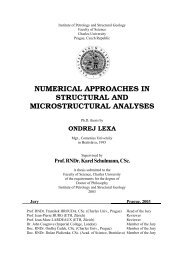
Figure 3-1: Rb–Sr data for the Agua Branca adamellite, Brazil,
plotted (a) on a conventional isochron diagram; and (b) on an
„improved“ isochron diagram after Provost (1990)
– 5 –

Vojtěch Janoušek:
Interpreting Sr–Nd isotopic data: numerical recipes
It is apparent from [2.1] and Fig. 3–1 that a corresponds to the initial ratio of the whole cogenetic suite
and the slope b of the isochron is expressed as:
Giving a formula for isochron age:
The isochrons are usually fitted using
software given in Tab. 3–1. The
algorithm utilizes weighted linear
regression and follows York (1969).
λt
( e −1)
b = tgα =
[3.2]
1
t = ln b +
λ
( 1)
Isochron
Provost (1990) France Pascal
IsoPlot Ludwig (1993) USA QuickBasic
[3.3]
Exercise 3-1
Table 3-1: Software used for geochronological calculations
[ISOCHRON.EXE]
The Rb–Sr isotopic composition of the Serra do Acari granite from Pará, Brazil, was determined by Xafi da
Silva et al. (1985). We will use this granite as a case study showing how isochrons are plotted, as well as how
isochron ages and initial ratios are obtained.
Calculate the age and Sr initial ratio for the Acari granite using simple linear
regression (MS Excel). Then calculate the same parameters using weighted linear
regression implemented by Provost (1990) and produce both conventional and
improved isochron plots. Compare results obtained in both cases. Which sample controls the
regression and why
Sample
87 Rb/ 86 Sr 1σ
87 Sr/ 86 Sr 1σ
AT-R-173 5.743 0.062 0.858993 0.000034
AT-R-167 22.290 0.280 1.290200 0.000050
AT-R-157 42.170 0.530 1.760370 0.000069
AT-R-165 61.230 0.980 2.248950 0.000140
AT-R-158 99.000 1.800 3.182530 0.000170
AT-R-169 232.000 3.300 6.548880 0.000470
[acari.xls, acari.sr]
Hints:
! Plot a diagram analogous to Figure 3–1a (if you dare, you can even plot error bars),
! Fit the data by linear regression,
! Intercept of the regression line equals to the sought initial ratio,
! Age can be calculated from the slope using eq. [3.3],
! Start ISOCHRON.EXE, import the data file provided on the floppy (acari.sr),
! Note the format of the *.SR data file: first line is ignored and is intended for
comments, the following lines contain: sample_number, 87 Rb/ 86 Sr, 1σ, 87 Sr/ 86 Sr and
1σ with several spaces in between,
! If in doubt, just press ENTER to accept the defaults offered by the program.
– 6 –

Vojtěch Janoušek:
Interpreting Sr–Nd isotopic data: numerical recipes
4. EPSILON ND VALUES
The isotopic evolution of Nd in the Earth is described
in terms of a model, called CHUR (Chondritic
Uniform Reservoir: DePaolo, 1988), which is
assumed to have Sm/Nd ratio equal to that of
chondrites. This model is widely used for comparison
of initial isotopic composition of a studied (usually
igneous) rock with that of primitive mantle at the time
of its generation. This is done by means of the ε-
notation:
⎛
λt
( e −1)
λ
( e −1)
0 0
t
SA SA
4
ε = ⎜
−1
× 10
0
0
⎟
CHUR
[4.1]
t
I
CHUR
− RCHUR
⎝
I
− R
Where:
t refers to the time of the intrusion,
0 to the present,
SA = sample,
present-day composition of CHUR is:
147 Sm/ 144 Nd = 0.1967
143 Nd/ 144 Nd = 0.512638
(Jacobsen & Wasserburg, 1980).
⎞
⎠
Partial melting
CHUR
Residual solid (DM)
CHUR
Partial melt
T 0
Time
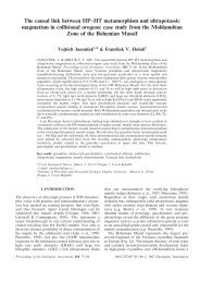
Figure 4-1: Isotopic evolution of Nd in a chondritic
uniform reservoir (CHUR), igneous rock formed by
its partial melting and the residual solid (after
Faure, 1986)
Partial melting of CHUR would produce
melts with Sm/Nd ratios lower than
CHUR (as Nd is more incompatible than
Sm). On the other hand, the residue will
be relatively enriched in Sm and have a
higher Sm/Nd ratio (Fig. 4–1). This
means that old igneous rocks formed by
CHUR-like mantle melting should have
present-day 143 Nd/ 144 Nd generally lower
than CHUR and mantle domains depleted
in melt will, with time, develop
143 Nd/ 144 Nd ratios higher than CHUR.
In general, if the ε Nd value is
negative, the rock is thought to having
been derived from (or assimilated a great
proportion of) a material with Sm/Nd
ratio lower than CHUR (e.g. old crustal
rocks — Fig. 4–2). If, in turn, the ε Nd
value is positive, then the rock came
from a source with high time-integrated
Sm/Nd ratio, such as residual mantle
domains depleted in incompatible
elements during a previous partial
melting event (so-called Depleted
Mantle, DM — DePaolo, 1988).
Figure 4-2: Tentative Sr–Nd correlation diagram showing
the approximate compositions of the most common crustal
and mantle rocks (after Rollinson, 1993)
– 7 –

Vojtěch Janoušek:
Interpreting Sr–Nd isotopic data: numerical recipes
Exercise 4-1
Calculate initial ε Nd values for the granitoid samples from the Central Bohemian
Pluton (see exercises 1–1 and 2–1) assuming that their age is 350 Ma. Plot the initial
87 Sr/ 86 Sr ratios and ε Nd values into a diagram similar to Fig. 4–2 and briefly discuss the
possible sources of individual granitoid bodies, provided no assimilation, magma mixing or later
disturbance of the Sr–Nd isotopic system has taken place.
[cbp.xls]
Hints:
! Epsilon values are calculated using eq. [4.1],
! Note that the intersection of both axes will be in ε Nd = 0 and the 87 Sr/ 86 Sr composition
of UR 350 Ma ago (see Page 2 for constants),
! Having trouble with interpretation See Figure 4–2.
5. ND MODEL AGES
Single-stage ages
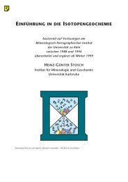
The single-stage Nd model ages provide an estimate
of the time that a rock unit has had a different Sm/Nd
ratio from that of the Earth’s mantle (represented by a
model reservoir, typically either DM or CHUR:
Fig. 5–1). The equation
I = ( 143 Nd/ 144 Nd)
SA Sample
DM Depleted mantle
I 0 DM
I 0 SA
I = I
[5.1]
T
SA
T
DM
SAMPLE
is solved for T (the so-called model age):
I T = I T
DM SA
I
0
SA
− R
0
SA
λT
0 0 λT
( e −1) = I − R ( e −1)
DM
DM
[5.2]
DM
Partial melting
T 0
T
Nd
DM
0 0
1 ⎛ I ⎞
SA
− I
DM
= ln
⎜ + 1
⎟
0 0
λ ⎝ RSA
− RDM
⎠
[5.3]
Time
Figure 5-1: Theoretical concept of a single-stage
Nd model age. Model age is the time in the past,
when mantle evolution line (here is assumed
depleted mantle) intersects with that for the given
sample.
– 8 –

Vojtěch Janoušek:
Interpreting Sr–Nd isotopic data: numerical recipes
Two-stage ages
The Nd model ages can be also calculated using the
two-stage model of Liew and Hofmann (1988) which
accounts for the fact that a great deal of rocks contain
a significant proportion of a crustally-derived
material. In the following formulae, the indexes DM,
CC, SA refer to depleted mantle, average crustal
reservoir and the sample, respectively. T = two-stage
Nd model age, t = crystallization age of the sample,
0 refers to the present day (Fig. 5–2). As:
I
0
CC
− R
0
CC
I = I
[5.4]
T
CC
T
DM
λT
0 0 λT
( e −1) = I − R ( e −1)
DM
DM
0 0
1 ⎛ I
⎞
CC
− I
DM
T = ln
⎜ + 1
⎟
0 0
λ ⎝ RCC
− RDM
⎠
For the crustal and sample evolution lines:
t
I = I
and because:
I
0
CC
CC
I
t
SA
= I
= I
0
SA
0
CC
0
SA
t
CC
[5.5]
[5.6]
− R
− R
0
CC
0
SA
I = I
−
λt
( e −1)
λt
( e −1)
t
SA
λt
0 0
( e − )( R − R )
1
SA CC
From [5.6] and [5.10]) we finally get :
0 λt
0 0 0
Nd 1 ⎛ I − ( −1)( − ) −
( ) ⎟ ⎞
SA
e RSA
RCC
I
DM
T = ln
⎜
DM
+ 1
0 0
λ ⎝ RCC
− RDM
⎠
Where:
I t = I t
SA CC
I T = I T
DM CC
I = ( 143 Nd/ 144 Nd)
⎛143 Nd⎞ 0
⎜ ⎟
⎝144 Nd ⎠DM = 0.513151 ⎝ ⎜⎛ 147 Sm
144 ⎠ ⎟⎞ 0
Nd DM = 0.219 ⎝ ⎜⎛ 147 Sm
144 ⎠ ⎟⎞ 0
Nd CC = 0.12
DM
CC
SA
DM
Depleted mantle
Average crust
Sample
CC
SAMPLE
T t 0
Time
Partial melting
Figure 5-2: Theoretical concept of a two-stage Nd
model age. An intermediate reservoir with Sm/Nd
ratio of typical crustal rocks (CC) is assumed.
I 0 DM
I 0 CC
I 0 SA
[5.7]
[5.8]
[5.9]
[5.10]
[5.11]
Exercise 5-1
Calculate single-stage T Nd and two-stage TNd model ages for the granitoid samples
CHUR DM
from the Central Bohemian Pluton, in the second case assuming the intrusion age of
350 Ma.
Hints:
[cbp.xls]
! Necessary parameters of both models are given on Page 2,
! Single-stage CHUR Nd model ages are obtained using eq. [5.3],
! Two-stage DM Nd model ages are calculated by eq. [5.11].
– 9 –

Vojtěch Janoušek:
Interpreting Sr–Nd isotopic data: numerical recipes
6. BINARY MIXING
A. Major and trace elements
Mixing of two components, A, B. For fraction f of the
component A:
f
A
=
A+
B
Concentration of any element in the mixture is:
M
A
B
A
B
B
[6.1]
c = c f + c ( 1−
f ) = f ( c − c ) + c [6.2]
For two elements, X and Y (Faure, 1986):
Y
M
=
X
M
( YA
− YB)
Y X
+
( X − X ) X
A
B
− Y X
− X
B A A B
which is an equation of a straight line on the X–Y plot.
A
B
[6.3]
A1 Major-element based mixing test
Equation [6.2] corresponds to a straight line in the
diagram of c A –c B versus c M –c B with the slope being
equivalent to the proportion of the component A (mixing
test sensu Fourcade and Allègre, 1981 — see Fig. 6–1a).
20
10
-10
3
2
1
0
0
c -c
M B
Na
K Al
Ti
Mn
Fe 2+ Fe3+
Ca
Mg
cA-cB
-10 0 10
20
HYBRID/ BASIC
Ba Rb Sr Zr Hf La Ce Y Ni Co
Si
b
a
Cr
A2 Trace-element based mixing test
Castro et al. (1990) used the theoretical proportions
obtained from the major-element based mixing test for
calculation of theoretical contents of trace-elements in
the suspected hybrid. Then they compared the calculated
and observed trace-element contents (see Fig. 6–1b).
Although eq.[6.2] should also work for the trace
elements, it must be borne in the mind that the
fractionation following the magma-mixing could
Figure 6-1: Mixing test for the Kozárovice
quartz monzonite (Janoušek et al. – in
print; presumed end-members Kozárovice
granodiorite and associated monzogabbro).
The trace–element diagram (b) compares
the actual composition of the hybrid (filled
symbols) with calculated composition
(empty symbols) using proportions from the
mixing test for the major elements (see
Exercise 6–1).
have dramatically altered the original trace–element contents. Therefore incompatible
elements should be preferably used for this purpose.
Exercise 6-1
In the Central Bohemian Pluton, associated with the Kozárovice granodiorite are K-rich pyroxene- and
amphibole-bearing monzonitic rocks (e.g. Lučkovice melamonzonite–monzogabbro). In a quarry SE of
Kozárovice small bodies of biotite–amphibole quartz monzonite occur, whose hybrid origin is strongly
supported by both the field evidence and presence of disequlibriun textures on a mineral scale.
– 10 –

Vojtěch Janoušek:
Interpreting Sr–Nd isotopic data: numerical recipes
Using major-element compositions given below, test whether the quartz monzonite
could have originated by magma mixing between Kozárovice granodiorite and
Lučkovice monzogabbro. Given that the granodiorite contains 1154 ppm and the
monzogabbro 2329 ppm Ba, calculate the expected Ba concentration in the quartz monzonite.
A: Kozárovice
granodiorite
M: Quartz monzonite B: Lučkovice
monzogabbro
SiO 2 64.60 59.58 49.21
TiO 2 0.57 0.72 1.02
Al 2 O 3 14.99 14.8 13.69
FeO 2.79 4.08 6.96
Fe 2 O 3 1.27 1.69 2.47
MnO 0.08 0.14 0.15
MgO 2.37 4.11 8.53
CaO 3.44 5.33 9.74
Na 2 O 3.12 2.84 1.89
K 2 O 4.34 4.19 3.61
[koza.xls]
Hints:
! Plot a diagram analogous to Figure 6–1a,
! Fit the data by linear regression (forcing the intercept to zero),
! The quality of the fit is shown by the correlation coefficient,
! Slope of the regression line gives the proportion of the acid end-member,
! For this value of f, calculate the Ba contents in the mixture using eq. 6.2.
B. Radiogenic isotopes (after Faure, 1986)
B1 Using a single isotopic ratio
The mixing equation for the isotopic ratios is:
I
M
= I
A
⎛ c
⎜
⎝ c
A
M
f ⎞
⎟ + I
⎠
B
⎛ c
⎜
⎝
B
(1 −
c
Eqs [6.2] and [6.4] can be, after eliminating f, developed into:
M
f ) ⎞
⎟
⎠
[6.4]
I
M
c c
c
B
( I
B
− I
A
) c
AI
A
− cB
+
( c
A
− cB
) c
A
− cB
A
B
= [6.5]
M
I
and this is an equation of a hyperbola in the c–I (e.g. Sr– 87 Sr/ 86 Sr) space.
In the isotope-based modelling of the binary mixing are frequently used plots such as 1/Sr–( 87 Sr/ 86 Sr) i
(i.e. age-corrected Sr isotopic ratios), where the mixing hyperbola changes into a straight line. For
suite of co-genetic rocks, a non-zero slope of this line implies that some sort of open process has
played a role, such as magma mixing or wall-rock contamination. On the other hand, samples that
– 11 –

Vojtěch Janoušek:
Interpreting Sr–Nd isotopic data: numerical recipes
originated from the same magma by various degrees of fractional crystallization only preserve
identical initial isotopic ratios (forming horizontal lines).
Eqs [6.2] and [6.4] can be, after eliminating c M , combined into a formula for f. The parameter f can
be calculated if the isotopic compositions and element concentrations for both end-members as well as
the isotopic composition of the presumed hybrid are known:
f
=
I
M
( c
A
cB
− c
( I − I )
B
B
) − I
A
M
c
A
+ I
B
c
B
[6.6]
Exercise 6–2
Plot the theoretical mixing hyperbola between granite and basalt, whose compositions
are given below. Calculate the 87 Sr/ 86 Sr ratio of a mixture, containing 50 % of the
granite. Calculate proportion of the granite in a mixture that has 87 Sr/ 86 Sr = 0.71200.
A: granite B: basalt
Sr 160 ppm 318 ppm
87 Sr/ 86 Sr 0.73691 0.70362
Hints:
! Calculate the Sr concentrations (eq. [6.2]) and isotopic composition (eq. [6.4]) of the hybrid
for various proportions of the granite (f = 0–1)
! Plot the results in the Sr– 87 Sr/ 86 Sr diagram
! Check the results in the 1/ Sr– 87 Sr/ 86 Sr plot — they should form a straight line
! Proportion f of the granite end-member is obtained using eq. [6.6].
B2 Using a pair of different isotopic ratios (Sr–Nd)
Taking into account that [6.2]
c = c f + c ( 1−
f )
M
A
B
the equation [6.4] can be rewritten as:
I
Ac
A
f + I
BcB
(1 − f )
I
M
= [6.7]
c f + c (1 − f )
A
Both Sr and Nd isotopic compositions can be calculated for pre-set values of the parameter f and the
corresponding mixing hyperbola plotted in the 87 Sr/ 86 Sr – 143 Nd/ 144 Nd space.
General equation of this mixing hyperbola is derived from two equations [6.7], one for Sr and one for
Nd, by solving both equations for f and equating the results:
B
– 12 –

Vojtěch Janoušek:
Interpreting Sr–Nd isotopic data: numerical recipes
⎛
A⎜
⎝
87
86
where:
87
Sr ⎞ Sr
⎟ + B
⎛ 86
Sr ⎠ ⎝ ⎜ ⎞
⎟
Sr ⎠
143
143
Nd
Nd
A = ⎛ Nd
BSr
144
A 144
⎝ ⎜ ⎞
⎟ − ⎛
Nd ⎠ ⎝ ⎜ ⎞
⎟
Nd ⎠
B = Nd Sr − Nd Sr
87
87
Sr
Sr
C = ⎛ Nd
BSr
86
A 86
⎝ ⎜ ⎞
⎟ − ⎛
Sr ⎠ ⎝ ⎜ ⎞
⎟
Sr ⎠
143
Nd
D = ⎛ 144
⎝ ⎜ ⎞
⎟ ⎛ Nd ⎠ ⎝ ⎜
143
Nd ⎞ Nd
⎟ + C
⎛ D 0
144
Nd ⎠ ⎝ ⎜ ⎞
⎟ + =
Nd ⎠
144
M M M M
B
A B B A
A
A
87
86
Nd Sr
Nd Sr
143
Sr ⎞
Nd
⎟ Nd
ASrB
− ⎛ 144
Sr ⎠ ⎝ ⎜ ⎞
⎟
Nd ⎠
B
⎛
⎜
⎝
143
B
A
A
A
B
B
B
⎛
⎜
⎝
87
Sr ⎞
⎟
⎠
86 Sr
A
Nd Sr
B
A
[6.8]
Straight line is obtained for a special case when B = 0, i.e.
( Sr / Nd)
( Sr / Nd)
A
B
= 1 [6.9]
Exercise 6-3
Plot the theoretical mixing hyperbola between granite and basalt in the 87 Sr/ 86 Sr–
143 Nd/ 144 Nd isotopic correlation diagram. Calculate 87 Sr/ 86 Sr and 143 Nd/ 144 Nd ratios of a
mixture containing 60 % of the granite. Compositions of the end members are:
A: granite B: basalt
Sr 160 ppm 318 ppm
87 Sr/ 86 Sr 0.73691 0.70362
Nd 31 ppm 18 ppm
143 Nd/ 144 Nd 0.51212 0.51300
Hints:
[mix.xls]
! Likewise in the previous example, calculate Sr and Nd isotopic compositions of the presumed
hybrid for various proportions of the granite (eq.[6.4]),
! The isotopic compositions of the hybrid for various values of f are obtained using eq. [6.7],
! Plot the results in the 87 Sr/ 86 Sr– 143 Nd/ 144 Nd diagram,
! Check the results in the 1/ Nd– 143 Nd/ 144 Nd plot – they should form a straight line.
– 13 –

Vojtěch Janoušek:
Interpreting Sr–Nd isotopic data: numerical recipes
CITED REFERENCES AND FURTHER READING
Textbooks an monographs in bold, asterisks indicate the (inevitably subjective) importance of the
given reference
** Albarède, F. (1995): Introduction to the Geochemical Modeling. — Cambridge University Press, pp. 1–
543.
** Arndt, N.T.; Goldstein, S.L. (1987): Use and abuse of crust-formation ages. Geology 15, 893–895.
* Bowen, R. (1988): Isotopes in Earth Sciences.– Elsevier, London, pp. 1–647.
** DePaolo, D.J. (1988): Neodymium isotope geochemistry.– Springer, Berlin, pp. 1–187.
** Dickin, A.P. (1995): Radiogenic Isotope Geology.– Cambridge University Press, Cambridge, pp. 1–452.
** Faure, G. (1986): Principles of Isotope Geology.– J. Wiley & Sons, Chichester, pp. 1–589.
* Fourcade S, Allègre CJ (1981) Trace elements behavior in granite genesis: a case study. The calc-alkaline
plutonic association from the Querigut Complex (Pyrénées, France). Contrib. Mineral. Petrol. 76: 177–
195.
** Geyh, M.A.; Schleicher, H. (1990): Absolute age determination.– Springer Verlag, Berlin, pp. 1–503.
* Hradetzky, H.; Lippolt, H.J. (1993): Generation and distortion of Rb–Sr whole-rock isochrons — effects of
metamorphism and alteration.– Eur. J. Mineral., 5, 1175–1193.
* Jacobsen, S.B., Wasserburg, G.J. (1980) Sm–Nd evolution of chondrites. Earth Planet. Sci. Lett. 50, 139–155.
Janoušek V, Rogers G, Bowes DR (1995) Sr–Nd isotopic constraints on the petrogenesis of the Central
Bohemian Pluton, Czech Republic. Geol. Rdsch. 84: 520–534.
** Kullerud, L. (1991): On the calculation of isochrons.– Chem. Geol. (Isotope Geoscience Section), 87, 115–124.
* Liew, T.C.; Hofmann, A.W. (1988): Precambrian crustal components, plutonic associations, plate environment
of the Hercynian Fold Belt of central Europe: indications from a Nd and Sr isotopic study. Contrib.
Mineral. Petrol. 98, 129-138.
** Ludwig, K.R. (1993): Isoplot, a plotting and regression program for radiogenic-isotope data, version 2.60.– US
Geological Survey Open-File Report 91–445, pp. 1–40.
** Lugmair, G.W.; Marti, K. (1978): Lunar initial 143 Nd/ 144 Nd: differential evolution line of the lunar crust and
mantle.– Earth Planet. Sci. Lett. 39, 349–357.
* Michard, A., Gurriet, P., Soudant, M.; Albaréde, F. (1985): Nd isotopes in French Phanerozoic shales: external
vs. internal aspects of crustal evolution.– Geochim. Cosmochim. Acta 49, 601–610.
** Provost, A. (1990): An improved diagram for isochron data.– Chem. Geol. (Isotope Geoscience Section), 80,
85–99.
** Rollinson, H.R. (1993): Using geochemical data: Evaluation, presentation, interpretation. Longman,
London, pp 1–352.
** Steiger, R.H., Jäger, E. (1977): Subcommission on geochronology: convention on the use of decay constants in
geo- and cosmochronology. Earth and Planetary Science Letters, 36, 359–362.
* Wasserburg, G.J., Jacobsen, S.B., DePaolo, D.J.; McCulloch, M.T.; Wen,T. (1981): Precise determination of
Sm/Nd ratios, Sm and Nd isotopic abundances in standard solutions Geochim. Cosmochim. Acta 45,
2311–2324.
** Wilson, M. (1989): Igneous Petrogenesis. Unwin Hyman, London, pp 1-466
Xafi da Silva, J.J., Alberto dos Santos, C., Provost, A. (1986): Granito Serra do Acari: geologia e implacação
metalogenética (folha Rio Mapuera, NW do estado do Pará). Proc. 2nd Symp. on Geology of Amazônia,
Belém, Vol. 2. Soc. Bras. Geol., São Paulo, pp. 93–109.
– 14 –

Vojtěch Janoušek:
Interpreting Sr–Nd isotopic data: numerical recipes
** York, D. (1969): Least-squares fitting of a straight line with correlated errors.– Earth Planet. Sci. Lett. 5,
320–324.
– 15 –