Harmonic Coordinates - Pixar Graphics Technologies
Harmonic Coordinates - Pixar Graphics Technologies
Harmonic Coordinates - Pixar Graphics Technologies

You also want an ePaper? Increase the reach of your titles
YUMPU automatically turns print PDFs into web optimized ePapers that Google loves.
<strong>Harmonic</strong> <strong>Coordinates</strong><br />
Tony DeRose Mark Meyer<br />
<strong>Pixar</strong> Technical Memo #06-02<br />
<strong>Pixar</strong> Animation Studios<br />
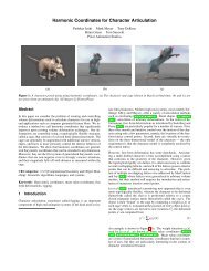
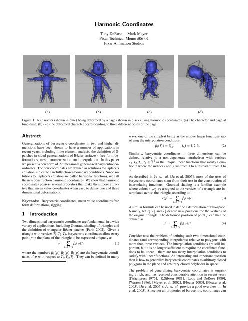
(a) (b) (c) (d)<br />
Figure 1: A character (shown in blue) being deformed by a cage (shown in black) using harmonic coordinates. (a) The character and cage at<br />
bind-time; (b) - (d) the deformed character corresponding to three different poses of the cage.<br />
Abstract<br />
Generalizations of barycentric coordinates in two and higher dimensions<br />
have been shown to have a number of applications in<br />
recent years, including finite element analysis, the definition of Spatches<br />
(n-sided generalizations of Bézier surfaces), free-form deformations,<br />
mesh parametrization, and interpolation. In this paper<br />
we present a new form of d dimensional generalized barycentric coordinates.<br />
The new coordinates are defined as solutions to Laplace’s<br />
equation subject to carefully chosen boundary conditions. Since solutions<br />
to Laplace’s equation are called harmonic functions, we call<br />
the new construction harmonic coordinates. We show that harmonic<br />
coordinates possess several properties that make them more attractive<br />
than mean value coordinates when used to define two and three<br />
dimensional deformations.<br />
Keywords: Barycentric coordinates, mean value coordinates,free<br />
form deformations, rigging.<br />
1 Introduction<br />
Two dimensional barycentric coordinates are fundamental in a wide<br />
variety of applications, including Gouraud shading of triangles and<br />
the definition of triangular Bézier patches [Farin 2002]. Given a<br />
triangle with vertices T1,T2,T3, barycentric coordinates allow every<br />
point p in the plane of the triangle to be expressed uniquely as<br />
p = ∑ βi(p)Ti<br />
(1)<br />
i=1,2,3<br />
where the numbers β1(p),β2(p),β3(p) are the barycentric coordinates<br />
of p with respect to T1,T2,T3. They can be defined in many<br />
ways, one of the simplest being as the unique linear functions satisfying<br />
the interpolation conditions:<br />
βi(Tj) = δi, j, i, j = 1,2,3. (2)<br />
Similarly, barycentric coordinates in three dimensions can be<br />
defined relative to a non-degenerate tetrahedron with vertices<br />
T1,T2,T3,T4 ∈ ℜ 3 as the unique linear functions that satisfy Equation<br />
2 where the indices i and j run from 1 to 4 instead of from 1 to<br />
3.<br />
As described in Ju et. al. [Ju et al. 2005], most of the uses of<br />
barycentric coordinates stem from their use in the construction of<br />
interpolating functions. Gouraud shading is a familiar example<br />
where colors c1,c2,c3 assigned to the vertices of a triangle are interpolated<br />
across the triangle according to<br />
c(p) = ∑<br />
i=1,2,3<br />
βi(p)ci<br />
(3)<br />
A similar formula can be used to define a deformation of two-space.<br />
Namely, let T ′<br />
1 ,T ′<br />
2 and T ′<br />
3 denote new positions for the vertices of<br />
the original triangle. The deformed position of point p can then be<br />
defined as<br />
p ′ = ∑<br />
i=1,2,3<br />
βi(p)T ′<br />
i<br />
(4)<br />
Consider now the problem of defining such two dimensional coordinates<br />
(and corresponding interpolants) relative to polygons with<br />
more than three vertices. The interpolation conditions are still important,<br />
but it is no longer sufficient to require the coordinate functions<br />
to be linear – there are too many interpolation conditions to<br />
satisfy with linear functions. An interesting and important question<br />
then is how to generalize barycentric coordinates to arbitrary closed<br />
polygons in the plane and arbitrary closed polyhedra in space.<br />
The problem of generalizing barycentric coordinates is surprisingly<br />
rich, and has received considerable attention in recent years<br />
([Wachpress 1975], [R.Sibson 1981], [Loop and DeRose 1989],<br />
[Warren 1996], [Meyer et al. 2002], [Floater 2003], [Floater et al.<br />
2005], [Ju et al. 2005]). Ju et. al. provide a good overview in [Ju<br />
et al. 2005]. Since not all properties of barycentric coordinates can
(a) (d)<br />
(b) (e)<br />
(c) (f)<br />
Figure 2: Two dimensional generalized barycentric coordinates<br />
used to define deformations of two different objects (shown in blue)<br />
using cages (shown in black). The top row shows the cages and objects<br />
at ”bind” time. The second row shows modified cages and<br />
the corresponding deformed objects using mean value coordinates.<br />
The last row shows modified cages and deformed objects using harmonic<br />
coordinates. In the last two rows, the original undeformed<br />
object is shown in white. The two methods perform similarly for<br />
convex shapes. In the bipedal case, harmonic coordinates perform<br />
better in that the motion of cage points in the left leg does not influence<br />
points in the right leg.<br />
be retained in the generalization, the richness results from the many<br />
different ways the properties can be relaxed.<br />
We are particularly interested in using generalized barycentric coordinates<br />
for character deformation, as shown in Figure 1 and as<br />
described in Ju et. al [Ju et al. 2005]. In this application, an object<br />
to be deformed is positioned relative to a closed shape that we’ll call<br />
a cage. Examples are shown in Figures 1 and Figure 2. The object<br />
is then “bound” to the cage by computing generalized barycentric<br />
coordinates gi(p) of each object point p relative to the cage vertices<br />
Ci. As the cage vertices are moved to new locations C ′ i , the<br />
deformed points p ′ are computed from<br />
p ′ = ∑ i<br />
gi(p)C ′ i<br />
Of the various generalized barycentric coordinate formulations<br />
available, mean value coordinates [Floater 2003; Floater et al. 2005;<br />
Ju et al. 2005] are particularly useful in this application because:<br />
(5)<br />
• The cage that controls the deformation can be any simple<br />
closed polygon in two dimensions, and any simple closed triangular<br />
mesh in three dimensions.<br />
• The coordinates are smooth, so the deformation is smooth.<br />
• The coordinates reproduce linear functions, so the object<br />
doesn’t “pop” when it is bound. That is, the coordinates are<br />
such that setting C ′ i to Ci in Equation 5 results in p ′ reducing<br />
to p.<br />
A second example motivated by the articulation of bipedal characters<br />
is shown in the second column of Figure 2. Notice how the<br />
modified cage points on the leg on the left in Figure 2(e) influence<br />
the position of object points in the leg on the right. This occurs<br />
because mean value coordinates are based on Euclidean (straightline)<br />
distances between points of the cage and points of the object.<br />
Although the influence is noticeable in still images, the movement<br />
of points in the right leg when the left leg cage points is particularly<br />
striking in interactive use, as demonstrated in the accompanying<br />
video. The behavior of 3D mean value coordinates is similar, and is<br />
highly undesirable for the articulation of characters in feature film<br />
production.<br />
What is needed for character articulation is a form of generalized<br />
barycentric coordinates that adds the following properties to those<br />
enjoyed by mean value coordinates:<br />
• Non-negativity. This implies that object points move in the<br />
same direction as cage points; negative coordinates mean<br />
they can move in the opposite direction. Negativity of mean<br />
value coordinates is responsible for the right leg points in Figure<br />
2(e) moving in the opposite direction from the left leg cage<br />
points. Negativity is also responsible for the collapsing of the<br />
left leg points in Figure 2(e).<br />
• Interior locality. Informally, the coordinates should fall off<br />
as a function of the distance between cage points and object<br />
points as measured within the cage.<br />
In this paper we show that such coordinates can be produced as solutions<br />
to Laplace’s equation with appropriately chosen boundary<br />
conditions. Since solutions to Laplace’s equation are generically<br />
referred to as harmonic functions, we therefore call these coordinates<br />
harmonic coordinates, and the deformations they generate<br />
harmonic deformations. 1<br />
1.1 Previous work<br />
Laplace’s equation, harmonic functions, and harmonic maps have<br />
often been mentioned in previous constructions of barycentric coordinates<br />
in two dimensions. For instance, the “cotangent weights” of<br />
[Pinkhall and Polthier 1993] and [Meyer et al. 2002] can be derived<br />
from piecewise linear discretizations of Laplace’s equation. Similarly,<br />
Floater’s construction of mean value coordinates was motivated<br />
by the mean value theorem for harmonic functions. It is<br />
somewhat surprising to us that direct solution of Laplace’s equation<br />
has never been used to create generalized barycentric coordinates,<br />
but that seems to be the case.<br />
Another connection between Laplace’s equation and mean value<br />
coordinates comes from the motivation given in [Ju et al. 2005].<br />
They derive mean value coordinates starting with an interpolant<br />
they call the mean value interpolant. The mean value interpolant<br />
to a function f defined on a closed boundary works as follows. To<br />
1 Since each component of a harmonic deformation is a harmonic function,<br />
many texts refer to such deformations as harmonic maps. We prefer<br />
the term harmonic deformation because of the context in which they’re used<br />
in this paper.
p<br />
(a)<br />
x<br />
Figure 3: Mean value vs harmonic interpolation. (a) The straightline<br />
paths corresponding to mean value interpolation. (b) The<br />
Brownian paths corresponding to harmonic interpolation.<br />
compute a value for each interior point p, consider each point x on<br />
the boundary. Multiply f (x) by the reciprocal distance from x to<br />
p, then average over all x (see Figure 3(a)). This definition makes<br />
it clear that mean value coordinates involve straight-line distances<br />
irrespective of the visibility of x from p. An alternative interpolant<br />
that respects visibility is to average not over all straight-line paths,<br />
but rather to average over all Brownian paths leaving p, where the<br />
value assigned to each path is the value of f at the point the path first<br />
hits the boundary (see Figure 3(b)). Although this definition at first<br />
seems intractable to compute, it is a famous result from stochastic<br />
processes (c.f. [Port and Stone 1978], [Bass 1995]) that the interpolant<br />
thus produced (in any dimension) in fact satisfies Laplace’s<br />
equation subject to the boundary conditions given by f . 2<br />
2 Theory<br />
In this section we formalize the discussion of Section 1. Let C be<br />
a closed (not necessarily convex) volume in d dimensions with a<br />
piecewise linear boundary. Geometers call such shapes polytopes,<br />
but because we have specific uses in mind, we refer to these shapes<br />
instead as cages. In two dimensions, a cage is a region of the plane<br />
bounded by a closed polygon (such as the one shown in Figure 2),<br />
and in three dimensions a cage is a closed region of space bounded<br />
by planar (though not necessarily triangular) faces. For each of<br />
the vertices Ci of the cage, we seek a function hi(p) defined on C<br />
subject to the following conditions:<br />
1. Interpolation: hi(Cj) = δi, j.<br />
2. Affine-invariance: ∑i hi(p) = 1 for all p ∈ C.<br />
3. Strict generalization of barycentric coordinates: when C is a<br />
simplex, hi(p) is the barycentric coordinate of p with respect<br />
to Ci.<br />
4. Smoothness: The functions hi(p) are at least C 1 smooth.<br />
5. Non-negativity: hi(p) ≥ 0, for all p ∈ C.<br />
6. Linear reproduction: Given an arbitrary function f (p), the<br />
coordinate functions can be used to define an interpolant<br />
H[ f ](p) according to:<br />
H[ f ](p) = ∑hi(p) f (Ci) (6)<br />
i<br />
Following Ju et. al [Ju et al. 2005], we require H[ f ](p) to<br />
be exact for linear functions. As shown by Ju et. al, taking<br />
f (p) = p means that<br />
p = ∑hi(p)Ci (7)<br />
i<br />
which is the“non-popping” condition mentioned in Section 1.<br />
2 We thank [name omitted for review purposes] for pointing out this con-<br />
nection to us.<br />
p<br />
(b)<br />
7. Interior locality: We quantify the notion of interior locality<br />
introduced above as follows: interior locality holds, if, in addition<br />
to non-negativity, the coordinate functions have no interior<br />
extrema.<br />
Mean value coordinates possess all but two of these properties:<br />
namely, non-negativity and interior locality. We claim that coordinate<br />
functions satisfying all seven properties can be obtained as<br />
solutions to Laplace’s equation<br />
▽ 2 hi(p) = 0, p ∈ Int(C) (8)<br />
if the boundary conditions are carefully chosen.<br />
To gain some insight into how the boundary conditions are determined,<br />
we consider first the construction of harmonic coordinates<br />
in two dimensions. It will then be clear how the construction generalizes<br />
to d dimensions. For reasons that will soon become apparent,<br />
the appropriate boundary conditions for hi(p) in two dimensions are<br />
as follows. Let ∂ p denote a point on the boundary ∂C of C, then<br />
hi(∂ p) = φi(∂ p),for all∂ p ∈ ∂C (9)<br />
where φi(∂ p) is the (univariate) piecewise linear function such that<br />
φi(Cj) = δi, j. For example, if C is the cage shown in Figure 4(a),<br />
then φi(∂ p) is the piecewise linear function defined on the edges<br />
e1,...,e15 such that φi(Cj) = δi, j, for i, j = 1,...,15.<br />
We now show that functions satisfying Equation 8 subject to Equation<br />
9 possess the properties enumerated above. It turns out that the<br />
linear reproduction property subsumes several other conditions, so<br />
for purposes of proof we verify the conditions in a different order<br />
than the one presented above.<br />
• Interpolation: by construction hi(Cj) = φi(Cj) = δi, j.<br />
• Smoothness: Away from the boundary harmonic coordinates<br />
are solutions to Laplace’s equation, and hence they are C ∞ .<br />
• Non-negativity: harmonic functions achieve their extrema at<br />
their boundaries. Since boundary values are restricted to [0,1],<br />
interior values are also restricted to [0,1].<br />
• Linear reproduction: Let f (p) be an arbitrary linear function.<br />
We need to show that H[ f ](p) = f (p), where H[ f ](p)<br />
is defined as in Equation 6. We begin by establishing that<br />
H[ f ](p) = f (p) everywhere on the boundary of C. If ∂ p is a<br />
point on the boundary of C, then by construction<br />
H[ f ](∂ p) = ∑hi(∂ p) f (Ci) = ∑φi(∂ p) f (Ci) (10)<br />
i<br />
i<br />
The functions φi(∂ p) are the univariate linear B-spline basis<br />
functions (commonly known as the “hat function” basis),<br />
which are capable of reproducing all linear functions on ∂C<br />
(in fact, they reproduce all piecewise linear functions on ∂C).<br />
Next we extend the result to the interior of C. Note that since<br />
f (p) is linear, all second derivatives vanish, and in particular<br />
▽ 2 f (p) = 0; thus f (p) satisfies Laplace’s equation on the<br />
interior of C. H[ f ](p) also satisfies Laplace’s equation on the<br />
interior, because for interior points ·p:<br />
▽ 2 H[ f ](·p) = ▽ 2 ∑ i<br />
= ∑ i<br />
= ∑ f (Ci)0<br />
i<br />
= 0<br />
hi(·p) f (Ci)<br />
f (Ci) ▽ 2 hi(·p)<br />
Since f (p) and H[ f ](p) agree on their boundaries and are<br />
both solutions to the same differential equation, by uniqueness<br />
of solutions to PDEs, they must be the same function.
e15<br />
C1<br />
C15<br />
e2<br />
e1<br />
C3<br />
C2<br />
(a) (b) (c)<br />
Figure 4: A comparison of coordinate functions for a concave cage. (a) A 2D cage with vertices C1,...,C15; (b) the value of the mean<br />
value coordinate for C2 (yellow indicates positive values, green indicates negative values); (c) the value of the harmonic coordinate for C2<br />
(red denotes the exterior of the cage where the function is undefined). To accentuate values near zero, intensities of yellow and green are<br />
proportional to the square root of the coordinate function value. The significant influence of the position of C2 on object points in the leg on<br />
the right is indicated by the presence of green in the right leg of (b). The corresponding influence in (c) is essentially zero.<br />
• Affine invariance: The function f (p) = 1 is linear, so affine<br />
invariance follows immediately from the linear reproduction<br />
property.<br />
• Strict generalization of barycentric coordinates. If the cage<br />
C consists of a single triangle harmonic coordinates reduce<br />
to barycentric coordinates. Let β j(p) denote the barycentric<br />
coordinates of p with respect to the triangle. To establish that<br />
h j(p) = β j(p), note that β j(p) is a linear function, so we can<br />
use the linear reproduction property above by taking f (p) =<br />
β j(p):<br />
β j(p) = H[β j](p)<br />
= ∑ i<br />
hi(p)β j(Ci)<br />
= ∑hi(p)δi, j<br />
i<br />
= h j(p)<br />
• Interior locality: follows from non-negativity and the fact that<br />
harmonic functions possess no interior extrema.<br />
To generalize from two to d dimensions, we first back up and consider<br />
harmonic coordinates in one dimension. In one dimension<br />
a cage is a line segment bounded by two vertices C0 and C1, and<br />
Laplace’s equation reduces to<br />
d2hi(p) = 0. (11)<br />
d p2 Thus, hi(p) is a linear function, and the proper (zero dimensional)<br />
boundary conditions come from the interpolation property:<br />
hi(Cj) = δi, j.<br />
With this insight, we can repose the two dimensional construction<br />
as: to construct two dimensional harmonic coordinates, start with<br />
the interpolation conditions hi(Cj) = δi, j. This determines the coordinates<br />
on the 0-dimensional facets (the vertices) of C. Next, extend<br />
the coordinates to the 1-dimensional facets (the edges) of C using<br />
the one dimensional version of Laplace’s equation. Finally, extend<br />
them to the two dimensional facets (the interior) of C using the two<br />
dimensional version of Laplace’s equation.<br />
The extension to three and higher dimensions follows immediately:<br />
The harmonic coordinates hi(p) for a d dimensional cage C with<br />
vertices Ci, are the unique functions such that:<br />
1. hi(Cj) = δi, j.<br />
2. On every facet of dimension k ≤ d, the k dimensional Laplace<br />
equation is satisfied.<br />
To prove that d dimensional harmonic coordinates defined in this<br />
way possess the required properties, we can use induction on the<br />
facet dimension, starting with the 1-facets as the base case. The<br />
proofs given above for two dimensions are actually more general;<br />
they are valid in any dimension k assuming that linear reproduction<br />
is achieved on the k − 1 facets. These proofs therefore serve as the<br />
inductive step.<br />
Having defined coordinates in this way, by construction we have<br />
the following additional property that is shared by barycentric coordinates<br />
and Warren’s [Warren 1996] construction:<br />
• Dimension reduction: d dimensional harmonic coordinates,<br />
when restricted to a k < d dimensional facet, reduce to k dimensional<br />
harmonic coordinates.<br />
For example, a three dimensional cage bounded by triangular facets<br />
possesses harmonic coordinates that reduce to barycentric coordinates<br />
on the faces. Similarly, a dodecahedral cage will have 3D<br />
harmonic coordinates that reduce to 2D harmonic coordinates on<br />
its pentagonal faces.<br />
3 Implementation<br />
Our current implementation of harmonic coordinates is limited to<br />
two and three dimensions. In both cases we use a simple hierarchical<br />
finite difference solver, though in principle any solution method<br />
for Laplace’s equation, such as a finite element method, could be<br />
used.<br />
Now for some details. First we’ll describe the non-hierarchial version<br />
of the solver. We’ll then describe the extension to the hierarchical<br />
solver. For each vertex Ci of the cage, we approximate hi(p)<br />
over the interior of the cage as follows:<br />
1. Allocate a regular grid of cells that is large enough to enclose<br />
the cage. We choose the grid to contain 2 s cells on a side. All<br />
two dimensional examples have been computed with s = 6;<br />
three dimensional examples use s = 7. Each grid cell contains<br />
a value, and a tag, where the tag is one of UNTYPED,<br />
BOUNDARY, INTERIOR, or EXTERIOR.<br />
2. Initialize the grid by:<br />
(a) Tag all cells as UNTYPED.
(b) Scan-convert boundary conditions into the grid, marking<br />
each scan converted cell with the BOUNDARY tag.<br />
In two dimensions, the function φi(p) as defined in Section<br />
2 is scan-converted into the grid. In three dimensionals,<br />
our implementation is currently restricted to triangular<br />
faces, meaning that the boundary values varying<br />
in a piecewise linear fashion. We therefore use a<br />
simple voxel-based triangle scan-converter in this stage.<br />
(c) Starting with one of the corner cells, flood fill the exterior,<br />
marking each visited cell with the EXTERIOR tag.<br />
The flood fill recursion stops when BOUNARY tags are<br />
reached. Since the boundary is closed, only the exterior<br />
cells are visited during this stage.<br />
(d) Mark remaining UNTYPED cells as INTERIOR with<br />
harmonic coordinate value equal to 0.<br />
3. Laplacian smooth: For each INTERIOR cell, replace the<br />
value of the cell with the average of the value of its neighbors.<br />
In 2D cells are considered to be 4-connected; in 3D they<br />
are considered to be 6-connected. This Laplacian smoothing<br />
step is performed iteratively until the termination criterion is<br />
reached. Our solver terminates when the average change to a<br />
cell drops below a specified threshold τ. All examples in this<br />
paper have used τ = 10 −5 .<br />
The solver described above can be significantly accelerated by noting<br />
that Laplace’s equation produces very smoothly varying functions.<br />
By first solving the problem at a lower resolution, better starting<br />
points for the iteration can be obtained. The hierarchical solver<br />
exploits this observation by “pulling” the boundary conditions up to<br />
a coarser level, recursively solving there, “pushing” the coarse solution<br />
down to the finer level, then iterating the Laplacian smoothing<br />
step until convergence is reached.<br />
The pulling step in two dimensions computes a coarse level grid of<br />
size 2 s−1 × 2 s−1 from a fine level grid of size 2 s × 2 s . Each coarse<br />
level grid cell represents four “children” cells on the finer level. In<br />
three dimensions, each coarse level grid cell represents eight children<br />
cells on the finer level. In both cases, a coarse cell is tagged<br />
as a BOUNDARY if at least one child is tagged as a BOUNDARY;<br />
it is tagged as EXTERIOR if all children are EXTERIOR, and it<br />
is tagged as INTERIOR if all children are INTERIOR. The value<br />
of a coarse level BOUNDARY cell is the average of the finer level<br />
BOUNDARY cells. INTERIOR cells on the coarse level are initialized<br />
with a value of zero.<br />
The pushing step propagates values from coarse level cells to IN-<br />
TERIOR cells on the finer level. Specifically, all INTERIOR cells<br />
on the finer level receive the value of their parent cell on the coarse<br />
level.<br />
4 Results<br />
The behavior of harmonic deformations in two dimensions is illustrated<br />
in the accompanying video as well as in Figure 2. The behavior<br />
of three dimensional harmonic deformations is illustrated in<br />
Figure 1, where we have bound an object containing 8019 vertices<br />
to a cage containing 112 vertices. The binding time for this example<br />
was 262 seconds, using the hierarchical solver with a finest<br />
grid with 2 7 cells on a side, and a coarsest grid with 2 4 cells on<br />
a side. The termination tolerance τ was 10 −5 . The corresponding<br />
bind time for mean value coordinates was 443 seconds using the<br />
algorithm as published in Figure 4 of [Ju et al. 2005].<br />
Notice that the bind time for harmonic coordinates is faster than<br />
that for mean value coordinates in this case. The primary reason is<br />
that the harmonic coordinate solver computes an entire coordinate<br />
Subdivisions Object vertices MVC (in sec) HC (in sec)<br />
0 21 0.16 29<br />
2 242 1.7 30<br />
4 3842 24 30<br />
5 15,362 113 30<br />
Table 1: A comparison of the binding time of the mean value<br />
and harmonic coordinate solvers as the number of object points increases.<br />
These examples were generated by using an icosahedron as<br />
the cage, and a subdivided dodecahedron as the object. The “Subdivisions”<br />
column indicates the number of times the dodecahedron<br />
was subdivided. Note that the time required for harmonic coordinates<br />
is relatively insensitive to the number of object vertices.<br />
function at a time. Once a coordinate function is computed it is<br />
very inexpensive to look up the value for each of the object points.<br />
The running time of the harmonic solver is therefore most strongly<br />
dependent on the number of cage vertices. The mean value solver,<br />
on the other hand, iterates over the entire cage for each of the object<br />
points. When the number of object points is small compared to<br />
the number of cage points, the mean value solver is faster. As the<br />
number of object points increases, the harmonic solver eventually<br />
outperforms the mean value solver. This trend is demonstrated in<br />
Table 1.<br />
One potential disadvantage of harmonic coordinates compared to<br />
mean value coordinates is memory overhead. A straightforward<br />
implementation of mean value coordinates requires only a constant<br />
amount of additional memory for each face of the cage, whereas the<br />
memory requirements of our simple harmonic solver is dominated<br />
by the solver grid. In two dimensions the grids are typically small<br />
(roughly 40Kbytes in our examples), but in three dimensions the<br />
grids can become rather large (roughly 25Mbytes in our examples).<br />
<strong>Harmonic</strong> coordinates computed as above are only numerical approximations,<br />
where the cell size and termination threshold determine<br />
the accuracy. The approximation error will, in general, cause<br />
each object point p to experience a residual ∆(p) when it is bound<br />
to the cage:<br />
∆(p) = p −∑ hi(p)Ci<br />
(12)<br />
i<br />
Another source of error occurs when coordinates below a threshold<br />
are removed from the sum, a process we call sparsification. Residuals<br />
due to sparsification occur for both mean value coordinates and<br />
harmonic coordinates. In cases where the residuals are too large,<br />
either because of an inaccurate solve or because of overly agressive<br />
sparisification, the residuals can be computed and stored at bind<br />
time on a per object point basis. They can then be added back at<br />
deformation time to improve the accuracy of the deformation with<br />
little run-time overhead. The examples used in this paper and the<br />
accompanying video were accurate enough that residuals were not<br />
used.<br />
4.1 Extension to cell complexes<br />
<strong>Harmonic</strong> coordinates as formulated thus far are defined relative to<br />
a cage consisting of a polytope, meaning the deformation is controlled<br />
entirely by boundary vertices of the cage. Once the behavior<br />
of the boundary is set, the behavior on the entire interior is completely<br />
determined. In many instances this is ideal. However, it<br />
is sometimes helpful to give artists additional control over interior<br />
details of the deformation. A simple example is shown in Figure 5<br />
where an additional isolated vertex has been added to refine control<br />
of the deformation in the area of the head of the character.<br />
It is also possible to extend the cage to include interior faces and<br />
edges; an example of including a collection of interior edges is
(a) (b)<br />
Figure 5: An example of interior control. (a) shows the cage and<br />
object at bind time, where an isolated interior vertex has been added<br />
to the cage; (b) shows the deformed object in response to movement<br />
of the interior vertex.<br />
shown in Figure 6. As demonstrated in this figure, the interior controls<br />
need not form a manifold — it is sufficient for the interior<br />
of the cage to form what is known as a linear cell complex. Intuitively,<br />
a linear cell complex is a collection of “cells” (vertices, linear<br />
edges, and planar faces) with the property that the intersection<br />
of any two cells is either empty or is another cell in the collection.<br />
<strong>Harmonic</strong> coordinates are easily adapted to such cages by treating<br />
the interior facets in exactly the same way as the bounary. 3<br />
Since harmonic functions are guaranteed to be only continuous at<br />
interior boundary conditions, harmonic coordinates are only C 0<br />
smooth across interior facets. In practice this means that if interior<br />
facets are used and smoothly deformed objects are desired, the<br />
interior facets should be placed so the object being deformed does<br />
not cross them.<br />
5 Summary<br />
We have provided a new and easy to implement construction for<br />
generalized barycentric coordinates as solutions to Laplace’s equation<br />
subject to carefully chosen boundary conditions — ones that<br />
correspond to lower dimensional solutions to Laplace’s equation.<br />
These harmonic coordinates improve on mean value coordinates in<br />
that they are guaranteed to be positive everywhere in the interior<br />
of the cage, and their influence falls off with distance as measured<br />
within the cage. Moreover, we have shown that the construction<br />
of harmonic coordinates can be carried out in any dimension, and<br />
we’ve show that the cage can be augmented with additional interior<br />
vertices, edges, and faces to provide more detailed control when<br />
necessary.<br />
Unlike mean value coordinates, harmonic coordinates are defined<br />
only within the cage, and they do not possess a closed form expression.<br />
The memory requirements of harmonic coordinates are also<br />
considerably larger than mean value coordinates, especially in three<br />
dimensions. However, we’ve show that they can be efficiently approximated<br />
using a hierarchical solver, and we’ve shown that in the<br />
common case where the number of object points greatly exceeds<br />
the number of cage points, they are faster to compute than mean<br />
value coordinates. Once coordinates have been computed, the cost<br />
of evaluating harmonic deformations is identical to that of deformations<br />
based on mean value coordinates.<br />
References<br />
BASS, R. 1995. Probabilistic Techniques in Analysis. Springer-<br />
Verlag.<br />
3 Note to reviewers: we have not yet implemented harmonic coordinates<br />
for cell complexes in 3D, but we will have such examples prior to final<br />
publication.<br />
(a)<br />
(b) (c)<br />
Figure 6: An example of interior control using a linear cell complex.<br />
(a) An object deformed using a cage with no interior controls.<br />
(b) the bind-time situation for the same object where an interior cell<br />
complex has been added to the cage. (c) the deformed object resulting<br />
from cage with interior controls. Note that the influence of the<br />
modified cage point is much more local in (c).<br />
FARIN, G. 2002. Curves and surfaces for CAGD: a practical guide,<br />
5th ed. Morgan Kaufmann Publishers Inc.<br />
FLOATER, M. S., KOS, G., AND REIMERS, M. 2005. Mean value<br />
coordinates in 3d. Computer Aided Geometric Design 22, 623–<br />
631.<br />
FLOATER, M. 2003. Mean value coordinates. Computer Aided<br />
Geometric Design 20, 1, 19–27.<br />
JU, T., SCHAEFER, S., AND WARREN, J. 2005. Mean value coordinates<br />
for closed triangular meshes. ACM Trans. Graph. 24, 3,<br />
561–566.<br />
LOOP, C. T., AND DEROSE, T. D. 1989. A multisided generalization<br />
of bézier surfaces. ACM Trans. Graph. 8, 3, 204–234.<br />
MEYER, M., LEE, H., BARR, A., AND DESBRUN, M. 2002. Generalized<br />
barycentric coordinates for irregular polygons. Journal<br />
of <strong>Graphics</strong> Tools 7, 1, 13–22.<br />
PINKHALL, U., AND POLTHIER, K. 1993. Computing discrete<br />
minimal surfaces and their conjugates. Experimental Mathematics<br />
2, 15–36.<br />
PORT, S. C., AND STONE, C. J. 1978. Brownian Motion and<br />
Classical Potential Theory. Academic Press.<br />
R.SIBSON. 1981. A brief description of natural neighbor interpolation.<br />
In Interpreting Multivariate Data, V. Barnett, Ed. John<br />
Wiley, 21–36.<br />
WACHPRESS, E. 1975. A Rational Finite Element Basis. Academic<br />
Press.<br />
WARREN, J. 1996. Barycentric coordinates for convex polytopes.<br />
Advances in Computational Mathematics 6, 97–108.