Getting a Handle on Advanced Cubic Equations of State

More documents

Recommendations

Info

long as the same alpha function (for pure-component vapor pressure correlation) and the same mixing rules (for mixtureproperty correlation) are used (5). Since the ability of any CEOS to predict phase equilibria of mixtures depends on the alpha function and the mixing rule, these two elements will be the focus of the remainder of this article. Alpha functions for cubic equations of state The accurate prediction of K-values from any CEOS requires an equally accurate prediction of pure-component vapor pressures, which depends on the development of an appropriate alpha function α(T). The first CEOS to be successfully applied to the calculation of thermodynamic properties for the vapor phase was the modified form of the van der Waals equation by Redlich and Kwong (6), who incorporated temperature dependence into the a term: P = RT v−b The success of the Redlich-Kwong (RK) equation stimulated numerous researchers to propose various correlations for improving the prediction of vapor pressure. Wilson (7) first introduced a general form of temperature dependence of the a parameter in the RK equation in 1964: a(T) = α(T)a c − 05 . aT vv ( + b) where a c is the value of a at the critical point. In 1966, Wilson (8) expressed α(T) as a function of the reduced temperature, T r = T/T c , and the acentric factor ω as follows: α(T) = T r + (1.57 + 1.62ω)(1 – T r ) (4) However, since the error of predicted vapor pressure from Eq. 4 is quite large, Wilson’s function did not find widespread use. The α(T) function that did find its way into the mainstream was proposed by Soave in 1972. He developed a linear equation for α as a function of temperature by plotting α 0.5 against T r 0.5 at a constant ω: α(T) = (1 + m(1 – T r 0.5)) 2 (5) The m parameter is obtained by forcing the equation to reproduce vapor pressures for light hydrocarbons corresponding to C 1 through C 10 at T r = 0.7, and is correlated as a function of ω: m = 0.480 + 1.57ω – 0.176ω 2 (6) ( 2) Soave’s development of Eqs. 5 and 6 represented a great step forward in the practical application of CEOS. The Soave α(T), (or Eq. 5) defined as a function of both T r and ω, is good for predicting the vapor pressures of hydrocarbons at temperatures above their normal boiling points, but not at conditions above the critical point, since the function does not decrease mono- (3) Nomenclature a, b = CEOS parameters a * , b * = reduced parameters of a and b A =Helmholtz energy c1 ,c2 ,c3 = constants in α(T) function (Eq. 14, 15) C1 = constant at infinite pressure Cr = constant at zero pressure Cv0 = function at zero pressure G = Gibbs energy k ij , k ij = binary interaction parameter = binary interaction parameter l ij m = parameter in Soave’s equation for α(T), Eq. 5 n = parameter in Soave’s expanded equation for α(T), Eq. 7 L, M, N = parameters in the Twu α function P = pressure R = ideal gas constant r = constant reduced liquid volume at zero-pressure T = temperature u, w = CEOS constants v = molar volume v 0 * = reduced liquid volume at zero pressure V = total volume x = mole fraction of component i in liquid phase i Z = compressibility facto Greek letters α = CEOS alpha function δ = parameter used to define τ ω = acentric factor τ = parameter used in TST excess Gibbs energy model Subscripts 0 = zero pressure ∞ = infinite pressure c = critical property i, j ,k = property of component i, j, k ij, ji = interaction property between components i and j ik, ki = interaction property between components i and k r = reduced property vdw = van der Waals Superscripts * = reduced property E = excess property (0) and (1) = denotes value of α when ω = 0 and ω = 1 † Any consistent set of units is acceptable. tonically with increasing temperature. Another shortcoming of Soave’s α(T) function is that the calculated vapor pressures tend to diverge from the experimental ones at low temperatures. Therefore, Soave proposed a new α(T) function to improve vapor-pressure prediction by expanding Eq. 5 as follows (9): α(T) = 1 + m(1 – T r )+n(1 – T r 0.5) 2 (7) where m and n are obtained by correlating vapor-pressure values generated by the Lee-Kesler EOS: m = 0.484 + 1.515ω – 0.44ω 2 (8) n = 2.756m – 0.700 (9) CEP November 2002 www.cepmagazine.org 59
Measurement & Control Unfortunately, the accuracy of predicting vapor pressure from Soave’s new α(T) was no better than the original one, and consequently, was never accepted for application. Numerous investigators have tried to improve Soave’s alpha function by either altering the parameters or adding extra terms. But as long as the same or a similar form of the alpha function is used, and the same approach as Soave is applied (i.e., plotting α 0.5 vs. T r 0.5), the function’s inherent weaknesswill not be overcome. Better vapor pressure prediction Twu et. al. (10, 11) developed a new methodology to improve the accuracy of the vapor-pressure prediction from a CEOS. They found that the alpha function is a linear function of the acentric factor at a constant reduced temperature. α = α (0) + ω(α (1) – α (0) ) (10) α ( ) ( ) 0 N M − 1 L ( 1− T ) = e r T r ( 1) ( 1) N M α () ( ) ( 1) ( 1) ( 1) 1 N M − 1 L ( 1− T ) = e r T r ( 0) ( 0) ( 0 ) ( 0 ) ( 0 ) N M ( 11) ( 12) The superscripts (0) and (1) in Eqs. 10, 11 and 12 are consistent with the definition of the acentric factor at ω = 0 and ω =1, respectively. In other words, these two alpha functions are forced to pass through the saturated vapor pressure at T r = 0.7 for ω = 0 and ω = 1, respectively. 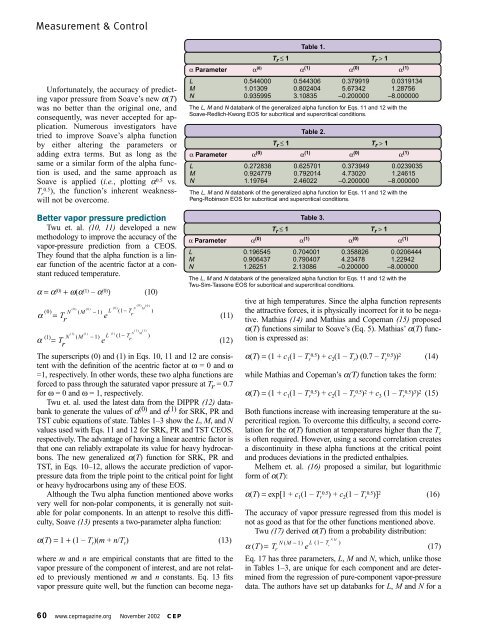Twu et. al. used the latest data from the DIPPR (12) databank to generate the values of α (0) and α (1) for SRK, PR and TST cubic equations of state. Tables 1–3 show the L, M, and N values used with Eqs. 11 and 12 for SRK, PR and TST CEOS, respectively. The advantage of having a linear acentric factor is that one can reliably extrapolate its value for heavy hydrocarbons. The new generalized α(T) function for SRK, PR and TST, in Eqs. 10–12, allows the accurate prediction of vaporpressure data from the triple point to the critical point for light or heavy hydrocarbons using any of these EOS. Although the Twu alpha function mentioned above works very well for non-polar components, it is generally not suitable for polar components. In an attenpt to resolve this difficulty, Soave (13) presents a two-parameter alpha function: α(T) = 1 + (1 – T r )(m + n/T r ) (13) where m and n are empirical constants that are fitted to the vapor pressure of the component of interest, and are not related to previously mentioned m and n constants. Eq. 13 fits vapor pressure quite well, but the function can become nega- 60 www.cepmagazine.org November 2002 CEP Table 1. Tr ≤ 1 Tr > 1 α Parameter α (0) α (1) α (0) α (1) L 0.544000 0.544306 0.379919 0.0319134 M 1.01309 0.802404 5.67342 1.28756 N 0.935995 3.10835 –0.200000 –8.000000 The L, M and N databank of the generalized alpha function for Eqs. 11 and 12 with the Soave-Redlich-Kwong EOS for subcritical and supercritical conditions. Table 2. Tr ≤ 1 Tr > 1 α Parameter α (0) α (1) α (0) α (1) L 0.272838 0.625701 0.373949 0.0239035 M 0.924779 0.792014 4.73020 1.24615 N 1.19764 2.46022 –0.200000 –8.000000 The L, M and N databank of the generalized alpha function for Eqs. 11 and 12 with the Peng-Robinson EOS for subcritical and supercritical conditions. Table 3. Tr ≤ 1 Tr > 1 α Parameter α (0) α (1) α (0) α (1) L 0.196545 0.704001 0.358826 0.0206444 M 0.906437 0.790407 4.23478 1.22942 N 1.26251 2.13086 –0.200000 –8.000000 The L, M and N databank of the generalized alpha function for Eqs. 11 and 12 with the Twu-Sim-Tassone EOS for subcritical and supercritical conditions. tive at high temperatures. Since the alpha function represents the attractive forces, it is physically incorrect for it to be negative. Mathias (14) and Mathias and Copeman (15) proposed α(T) functions similar to Soave’s (Eq. 5). Mathias’ α(T) function is expressed as: α(T) = (1 + c 1 (1 – T r 0.5) + c 2 (1 – T r ) (0.7 – T r 0.5)) 2 (14) while Mathias and Copeman’s α(Τ) function takes the form: α(T) = (1 + c 1 (1 – T r 0.5) + c 2 (1 – T r 0.5) 2 + c 3 (1 – T r 0.5) 3 ) 2 (15) Both functions increase with increasing temperature at the supercritical region. To overcome this difficulty, a second correlation for the α(T) function at temperatures higher than the T c is often required. However, using a second correlation creates a discontinuity in these alpha functions at the critical point and produces deviations in the predicted enthalpies. Melhem et. al. (16) proposed a similar, but logarithmic form of α(T): α(T) = exp[1 + c 1 (1 – T r 0.5) + c 2 (1 – T r 0.5)] 2 (16) The accuracy of vapor pressure regressed from this model is not as good as that for the other functions mentioned above. Twu (17) derived α(T) from a probability distribution: NM N( M − 1) L ( 1− T ) r r α ( T) = T e ( 17) Eq. 17 has three parameters, L, M and N, which, unlike those in Tables 1–3, are unique for each component and are determined from the regression of pure-component vapor-pressure data. The authors have set up databanks for L, M and N for a
Page 1: Measurement & Control Getti
Page 5 and 6: Measurement & Control the excess He
Page 7 and 8: Measurement & Control pendent throu

Getting a Handle on Advanced Cubic Equations of State

You also want an ePaper? Increase the reach of your titles

Delete template?

Save as template?