Atomic Force Microscopy in Cancer Cell Research - Clarkson ...
Atomic Force Microscopy in Cancer Cell Research - Clarkson ...
Atomic Force Microscopy in Cancer Cell Research - Clarkson ...

You also want an ePaper? Increase the reach of your titles
YUMPU automatically turns print PDFs into web optimized ePapers that Google loves.
CHAPTER 1<br />
<strong>Atomic</strong> <strong>Force</strong> <strong>Microscopy</strong> <strong>in</strong><br />
<strong>Cancer</strong> <strong>Cell</strong> <strong>Research</strong><br />
Igor Sokolov<br />
Department of Physics and Chemistry, <strong>Clarkson</strong> University, Potsdam, NY 13699, USA<br />
CONTENTS<br />
1.INTRODUCTION<br />
2007 by American Scientific Publishers' Inc. ISBN: 1-58883-071-3<br />
1. Introduction ............................................... 1<br />
1.1. Pr<strong>in</strong>ciples of AFM ........................................ 2<br />
1.2. Modes of AFM Operation .................................. 2<br />
1.3. Advantages of AFM <strong>in</strong> Biology ............................... 4<br />
2. AFM <strong>in</strong> Study of <strong>Cancer</strong> <strong>Cell</strong>s:General Overview ...................... 5<br />
2.1. AFM Detection of Surface Interactions (<strong>Atomic</strong> <strong>Force</strong> Spectroscopy) ....... 5<br />
2.2. <strong>Cell</strong>ular Sound (Sonocytology) ................................ 5<br />
2.3. <strong>Cell</strong> Mechanics .......................................... 6<br />
3. AFM <strong>in</strong> Study Mechanics of <strong>Cancer</strong> <strong>Cell</strong>s:Details ...................... 6<br />
3.1. Rigidity of <strong>Cell</strong>s:Where we are <strong>in</strong> Numbers ....................... 6<br />
3.2. How to Measure Rigidity of <strong>Cell</strong>s with AFM:Experimental Steps ......... 7<br />
3.3. How to Measure <strong>Cell</strong> Rigidity with AFM:Young’s Modulus Calculations .... 9<br />
3.4. Mechanics of <strong>Cancer</strong> <strong>Cell</strong>s:Results ............................ 10<br />
3.5. Discussion ............................................ 12<br />
4. Conclusions and Future Directions ............................... 14<br />
References ............................................... 15<br />
There is no need to describe the importance of study<strong>in</strong>g<br />
the problem of cancer. <strong>Atomic</strong> force microscopy (AFM) is<br />
a novel technique, aris<strong>in</strong>g out of and a form of scann<strong>in</strong>g<br />
probe microscopy (SPM), and which is one of the (if not<br />
the) major technique responsible for the emergence of modern<br />
nanotechnology. AFM has great potential <strong>in</strong> biology, <strong>in</strong><br />
particular, to study cells [1–49]. Therefore it is natural to<br />
try to understand what is done and what can be done with<br />
this technique to study cancer cells. This paper reviews the<br />
exist<strong>in</strong>g results of the study of cancer cells with AFM. The<br />
ma<strong>in</strong> focus is made on study<strong>in</strong>g the mechanics of cancer<br />
cells; <strong>in</strong> particular, <strong>in</strong> comparison with those of normal cells.<br />
ISBN:1-58883-071-3<br />
Copyright © 2006 by American Scientific Publishers<br />
All rights of reproduction <strong>in</strong> any form reserved.<br />
<strong>Cancer</strong> Nanotechnology<br />
Edited by Hari S<strong>in</strong>gh Nalwa and Thomas Webster<br />
Pages:1–17<br />
Although there are not many results as yet, it would be useful<br />
to present what we do know it <strong>in</strong> a systematic way, to<br />
summarize and to discuss future directions.<br />
Because AFM technique, <strong>in</strong> particular, the part of it that<br />
deals with force measurements, is still not very familiar to<br />
the broad community of scientists, we start from a brief<br />
description of the ma<strong>in</strong> pr<strong>in</strong>ciples of AFM. Then, we highlight<br />
the ma<strong>in</strong> advantages of us<strong>in</strong>g AFM <strong>in</strong> biology. After<br />
this <strong>in</strong>troduction, we will overview the ma<strong>in</strong> applications <strong>in</strong><br />
AFM <strong>in</strong> the study of cancer cells. The study of the mechanics<br />
of cancer cells, presumably one of the most promis<strong>in</strong>g<br />
areas of research, will be analyzed and discussed <strong>in</strong> detail.<br />
The necessity of such a detailed overview of AFM procedure<br />
is dictated by both the complexity of this technique and the<br />
<strong>Cancer</strong> Nanotechnology<br />
Edited by Hari S<strong>in</strong>gh Nalwa and Thomas Webster<br />
Pages:1–17
2 <strong>Atomic</strong> <strong>Force</strong> <strong>Microscopy</strong> <strong>in</strong> <strong>Cancer</strong> <strong>Cell</strong> <strong>Research</strong><br />
present state of research <strong>in</strong> this area. There are many different<br />
<strong>in</strong>terest<strong>in</strong>g results but without a unify<strong>in</strong>g protocol. One<br />
of the purposes of this review is to help develop such a<br />
protocol.<br />
1.1. Pr<strong>in</strong>ciples of AFM<br />
AFM is a relatively novel method. It was <strong>in</strong>vented <strong>in</strong> 1986<br />
as the first new extension of scann<strong>in</strong>g probe microscopy<br />
(which first appeared <strong>in</strong> 1981 <strong>in</strong> the guise of scann<strong>in</strong>g tunnel<strong>in</strong>g<br />
microscopy) [50]. Its technique is based on detection<br />
of forces act<strong>in</strong>g between a sharp probe, known as AFM tip,<br />
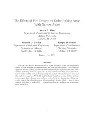
and the sample’s surface (Fig. 1). The tip is attached to<br />
a very flexible cantilever. Any motion of the cantilever is<br />
detected by various methods. The most popular is an optical<br />
system of detection. Laser light is reflected from the cantilever<br />
and detected by a photodiode. The tip is brought to<br />
contact or near-contact with the surface of <strong>in</strong>terest. Scann<strong>in</strong>g<br />
over the surface, AFM system records the deflection of<br />
the cantilever, due to very small forces between the atoms<br />
of the probe and the surface, with sub-nanometer precision.<br />
In pr<strong>in</strong>ciple, the whole system may look like just an oldfashioned<br />
stylus profilometer. Indeed, the only difference is<br />
the presence <strong>in</strong> AFM of a very sensitive detection system,<br />
microscopically sharp tips, and extremely high-precision tipsample<br />
position<strong>in</strong>g. The deflection signal (or any derivations<br />
of the deflection) is recorded digitally, and can be visualized<br />
on a computer <strong>in</strong> real-time.<br />
The AFM technique is much more than just simply<br />
microscopy. One can th<strong>in</strong>k about AFM tip as a microscopic<br />
“f<strong>in</strong>ger” with a nanosize apex. Follow<strong>in</strong>g this analogy, one<br />
can use such a f<strong>in</strong>ger to touch the surface to feel how rigid<br />
it is (rigidity force microscope or nano<strong>in</strong>denter); one can<br />
feel how sticky a surface is (chemical force microscopy);<br />
one can put some “goo” on the top of the tip, and consequently,<br />
detect how sticky the “goo” is with respect to the<br />
surface (functionalized tip imag<strong>in</strong>g); and so on. In essence,<br />
one can do with AFM correspond<strong>in</strong>gly what can be done<br />
with “a learn<strong>in</strong>g f<strong>in</strong>ger.” Depend<strong>in</strong>g on the sample and on<br />
<strong>in</strong>formation that one wishes to get, one can choose many<br />
different modes of operation of AFM.<br />
Laser source<br />
Photo detector<br />
sample surface<br />
Scann<strong>in</strong>g<br />
Figure 1. A schematic view of the AFM method.<br />
AFM cantilever<br />
1.2. Modes of AFM Operation<br />
Here we briefly describe a few basic modes which one can<br />
operate an AFM <strong>in</strong>:contact, tapp<strong>in</strong>g, and force mode. There<br />
are a few other modes of operation, which are not that popular<br />
as yet, and will not be described here. An advanced,<br />
so-called force-volume mode, which is rather useful for the<br />
study cell mechanics, will also be presented. All modes work<br />
<strong>in</strong> ambient conditions, as well as <strong>in</strong> liquids, <strong>in</strong>clud<strong>in</strong>g biological<br />
buffers. Comparative advantages and disadvantages of<br />
these modes are also described below.<br />
1.2.1. Contact Mode<br />
In contact mode, AFM tip is <strong>in</strong> actual contact with the sample’s<br />
surface. In pr<strong>in</strong>ciple, AFM <strong>in</strong> this mode can work precisely<br />
as described above. However, if there is a bump on<br />
the surface, the cantilever will be deflected more, and consequently,<br />
AFM tip scans over the surface with more force.<br />
This can result <strong>in</strong> scratch<strong>in</strong>g the sample surface. Moreover,<br />
if the sample surface has a trench, the cantilever may<br />
simply “fly over” without touch<strong>in</strong>g it. Both cases are not<br />
good. To exclude these bad behaviors of the cantilever, a<br />
positive-feedback system was <strong>in</strong>troduced. This works as follows.<br />
When the tip comes across a bump on the surface,<br />
the deflection of the cantilever <strong>in</strong>creases, and the feedback<br />
system elevates the whole cantilever holder so that the cantilever’s<br />
deflection is adjusted back to its orig<strong>in</strong>al value, and<br />
the cantilever is returned to its orig<strong>in</strong>al position. In the case<br />
of a trench, the same feedback system moves the cantilever<br />
down to aga<strong>in</strong>, ma<strong>in</strong>ta<strong>in</strong> the same deflection. This provides<br />
the same so-called “load force” between the tip and the<br />
sample.<br />
Pros of contact mode:<br />
• This is the simplest mode of operation. It requires m<strong>in</strong>imum<br />
operational skill and only basic hardware.<br />
• Allows very fast scann<strong>in</strong>g (typically 0.1–0.5 second per<br />
scan l<strong>in</strong>e).<br />
• The load force can be precisely controlled.<br />
• Good signal-to-noise ratio even <strong>in</strong> a noisy environment.<br />
• Generally cheaper and more robust cantilevers can be<br />
used.<br />
Cons of contact mode:<br />
• The tip can stretch or even scratch the surface. This<br />
will lead to artifacts, therefore disrupt<strong>in</strong>g the sample<br />
and lead<strong>in</strong>g to images and measurements that are not<br />
representational of the orig<strong>in</strong>al sample.<br />
• The tip can remove poorly attached parts of the sample.<br />
Apart from just damag<strong>in</strong>g the surface, this can contam<strong>in</strong>ate<br />
the tip surface and prevent it from be<strong>in</strong>g used any<br />
further.<br />
• Can provide only limited <strong>in</strong>formation about the surface<br />
(compar<strong>in</strong>g to other modes).<br />
Because of its simplicity, contact mode is one of the most<br />
popular modes. Contact mode is typically the best on solid<br />
and well-fixed surfaces. It normally requires rather soft cantilevers<br />
(spr<strong>in</strong>g constant (a characteristic measure) <strong>in</strong> the<br />
range of 0.001–1 Nm −1 ).
<strong>Atomic</strong> <strong>Force</strong> <strong>Microscopy</strong> <strong>in</strong> <strong>Cancer</strong> <strong>Cell</strong> <strong>Research</strong> 3<br />
1.2.2. Tapp<strong>in</strong>g/AC/Intermittent Contact Mode<br />
To further m<strong>in</strong>imize the tip impact onto the surface, dynamic<br />
or <strong>in</strong>termittent contact mode, also commonly known as Tapp<strong>in</strong>g<br />
mode (a trademark of Veeco Instruments, Inc.), was<br />
<strong>in</strong>troduced. Another name use for this mode is AC mode.<br />
In this mode the tip “taps,” or oscillates up and down very<br />
fast, touch<strong>in</strong>g the sample surface for a very short period of<br />
time dur<strong>in</strong>g relatively slow lateral scann<strong>in</strong>g. This considerably<br />
decreases scratch<strong>in</strong>g (although it does not elim<strong>in</strong>ate it<br />
completely). While <strong>in</strong> contact mode cantilever deflection is<br />
detected and measured, <strong>in</strong> this mode the amplitude of oscillation<br />
is typically measured. Positive feedback works <strong>in</strong> a<br />
similar manner to contact mode, by keep<strong>in</strong>g amplitude constant<br />
while scann<strong>in</strong>g.<br />
Pros of <strong>in</strong>termittent contact mode:<br />
• The tip does not scratch the surface, thereby avoid<strong>in</strong>g<br />
artifacts. This is extremely important for soft samples.<br />
• The tip typically does not remove parts of the sample.<br />
• The Tapp<strong>in</strong>g regime allows the collection of various<br />
k<strong>in</strong>ds of <strong>in</strong>formation related to the properties of the<br />
surface material (phase contrast).<br />
Cons of <strong>in</strong>termittent contact mode:<br />
• Successful use of this mode requires extensive operational<br />
skill and additional hardware.<br />
• The load force typically cannot be precisely controlled,<br />
<strong>in</strong> particular <strong>in</strong> liquid environments.<br />
• To atta<strong>in</strong> good imag<strong>in</strong>g quality, expensive cantilevers<br />
must be used.<br />
• The mode does not allow for fast scann<strong>in</strong>g (typically<br />
0.5–2 seconds per scan l<strong>in</strong>e).<br />
Because of its nondestructive scann<strong>in</strong>g, tapp<strong>in</strong>g mode is<br />
a natural choice for the imag<strong>in</strong>g of soft biological surfaces.<br />
It normally requires rather stiff cantilevers (spr<strong>in</strong>g constants<br />
<strong>in</strong> the range of 1 Nm−1 and above).<br />
1.2.3. <strong>Force</strong> Mode<br />
<strong>Force</strong> mode not an imag<strong>in</strong>g mode; it is used to measure<br />
forces act<strong>in</strong>g between AFM tip and the surface of <strong>in</strong>terest<br />
at a specific po<strong>in</strong>t. In contrast to the previous modes, the<br />
cantilever does not move <strong>in</strong> lateral direction. The scanner<br />
goes up and down, elevat<strong>in</strong>g and approach<strong>in</strong>g the cantilever<br />
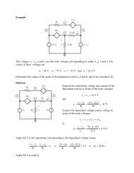
to the surface. As a result, the image shown <strong>in</strong> Figure 2 is<br />
a typical example of what is recorded. The force F of the<br />
bend<strong>in</strong>g of the cantilever (vertical axis) is plotted aga<strong>in</strong>st<br />
the vertical position z of the sample. When the tip is far<br />
away from the surface, there is no deflection, and consequently,<br />
the force is equal to zero (there is an assumption<br />
of no long-range forces). When the z position of the sample<br />
<strong>in</strong>creases (the sample is moved up by the scanner, Fig. 1),<br />
the tip-sample distance decreases. At some po<strong>in</strong>t, the tip<br />
touches the sample (position of contact). After that, the tip<br />
and sample move up together. This part of the force curve<br />
is called the region of constant compliance. At some po<strong>in</strong>t,<br />
which can be controlled by AFM operator, the sample stops<br />
and retracts down. The force curve before this po<strong>in</strong>t is called<br />
the tip-approach<strong>in</strong>g curve, or simply the approach<strong>in</strong>g curve.<br />
The force curve recorded when the sample is retracted down<br />
is known as the tip-retract<strong>in</strong>g curve, or simply the retract<strong>in</strong>g<br />
curve. Dur<strong>in</strong>g retraction the surface may display non-trivial<br />
Figure 2. A typical force–distance curve recorded by AFM <strong>in</strong> force<br />
mode. Both the approach<strong>in</strong>g and retract<strong>in</strong>g curves are shown.<br />
viscous and elastic properties. This typically results <strong>in</strong> hysteresis<br />
between the approach<strong>in</strong>g and retract<strong>in</strong>g curves, as<br />
shown <strong>in</strong> Figure 2.<br />
One more <strong>in</strong>terest<strong>in</strong>g feature of the retract<strong>in</strong>g curve is<br />
the non-zero force required to disconnect the tip from the<br />
surface. This is the so-called adhesion force. It appears due<br />
to weak short-range forces (such as van der Waals forces)<br />
act<strong>in</strong>g between the tip and surface while <strong>in</strong> contact.<br />
Pros of force mode:<br />
• Provides <strong>in</strong>formation about surface viscoelastic and<br />
elastic properties.<br />
• Also able to detect long-range forces.<br />
• Information about tip-surface adhesion force is<br />
recorded.<br />
Cons of force mode:<br />
• No topographical <strong>in</strong>formation is recorded.<br />
• Requires a very clean, homogeneous surface. Samples<br />
placed <strong>in</strong> biological buffers cannot be this clean.<br />
Moreover, biological surfaces are typically <strong>in</strong>tr<strong>in</strong>sically<br />
heterogeneous. To get reliable force <strong>in</strong>formation, one<br />
needs to collect and analyze a large amount of force<br />
curves.<br />
It is important to note about this mode that the absolute<br />
value of the force can be calculated with high precision.<br />
However, only the relative position of the sample can be<br />
well def<strong>in</strong>ed on the soft samples. This appears because of<br />
ambiguity <strong>in</strong> the def<strong>in</strong>ition of the tip-surface contact.<br />
To measure surface mechanics, one needs to choose a<br />
cantilever with the right spr<strong>in</strong>g constant, which should be of<br />
the same order of magnitude as the surface stiffness (surface<br />
spr<strong>in</strong>g constant).<br />
1.2.4. <strong>Force</strong>–Volume Mode<br />
This mode was <strong>in</strong>troduced [51] to solve the problems of<br />
force mode, described just above. As was noted <strong>in</strong> the previous<br />
section it is useful to simultaneously record the topology<br />
of the surface and force curves. Moreover, it is important<br />
to do multiple measurements to get reliable statistics. The
4 <strong>Atomic</strong> <strong>Force</strong> <strong>Microscopy</strong> <strong>in</strong> <strong>Cancer</strong> <strong>Cell</strong> <strong>Research</strong><br />
question is, how many measurements have to be done to<br />
get a def<strong>in</strong>ite answer for cell rigidity? While there is no any<br />
predef<strong>in</strong>ed answer to this question, one can estimate the<br />
amount of measurements to be 100 per cell. This has to be<br />
repeated for from 10 to 50 cells from a s<strong>in</strong>gle cell source,<br />
and ideally to do this for cells from three different sources.<br />
This results <strong>in</strong> 1,000 to 15,000 measurements. Obviously, this<br />
is impractical to do without automation.<br />
Moreover, it is impossible to determ<strong>in</strong>e the Young’s modulus<br />
of the sample (a measure of its stiffness, or, alternatively,<br />
its elasticity) without know<strong>in</strong>g the geometry of the<br />
surface near its contact with AFM tip. If the surface were<br />
ideally flat, then it would be irrelevant at what po<strong>in</strong>t to measure<br />
forces. In the case of biological cells, knowledge of<br />
geometry is important because cells are not necessarily flat.<br />
Therefore, one will need some k<strong>in</strong>d of automatic collection<br />
of data on forces and the geometry of the surface at the same<br />
time. This can be done <strong>in</strong> the so-called force–volume mode.<br />
“Classical” force–volume mode is implemented <strong>in</strong> many<br />
AFMs. There are different options regulat<strong>in</strong>g how this mode<br />
works. Below we describe only one of the most relevant<br />
set of options, <strong>in</strong> a typical set-up. While work<strong>in</strong>g <strong>in</strong> force–<br />
volume mode, AFM cantilever starts travel<strong>in</strong>g down from<br />
a def<strong>in</strong>ite distance away from the surface (known as the<br />
so-called ramp size), moves straight down (with no lateral<br />
motion) until the tip touches the surface, and the cantilever<br />
deflection reaches some def<strong>in</strong>ite level (called the trigger<br />
level). After that the motion of the cantilever is reversed.<br />
The AFM scanner pulls the cantilever straight back to a<br />
distance equal to the ramp size. Both the approach<strong>in</strong>g and<br />
retract<strong>in</strong>g curves are recorded dur<strong>in</strong>g such cycle. Then,<br />
still away from the surface at the ramp size distance, the<br />
tip advances <strong>in</strong> the lateral direction to a certa<strong>in</strong> distance,<br />
and force curves are aga<strong>in</strong> recorded, as described above.<br />
This operation cont<strong>in</strong>ues until the tip completes raster<strong>in</strong>g<br />
a square area of the sample. Topographical <strong>in</strong>formation <strong>in</strong><br />
such “scann<strong>in</strong>g” is also recorded because the trigger level<br />
(i.e., the required cantilever deflection) is reached faster on<br />
the hills and slower <strong>in</strong> the trenches.<br />
Thus, both topography and force curves are recorded at<br />
a number of po<strong>in</strong>ts, or pixels, over the sample surface. Typically<br />
this is recorded as a square matrix of, for example, 16 ×<br />
16, 32 × 32,or64× 64 pixels. The amount of <strong>in</strong>formation<br />
recorded <strong>in</strong> a s<strong>in</strong>gle force–volume file is generally limited.<br />
It means that each force curve can be recorded as a limited<br />
number of po<strong>in</strong>ts. In the Veeco Instruments Nanoscope<br />
software, up to version 5.12, the number of po<strong>in</strong>ts is limited<br />
to 512, 256, and 64 per force curve for 16 × 16, 32 × 32, and<br />
64 × 64 number of pixels, respectively. A newer version 6<br />
software allows work<strong>in</strong>g with up to 128 × 128 pixels for force<br />
curves recorded with 128 po<strong>in</strong>ts each. There are the follow<strong>in</strong>g<br />
advantages and disadvantages of this mode.<br />
Pros of force–volume mode:<br />
• It has all pros of the force mode.<br />
• Topographical <strong>in</strong>formation is recorded simultaneously<br />
with force curves.<br />
• It allows the collection of a large amount of data<br />
to ensure robust statistics. It does not require a very<br />
clean homogeneous surface. Therefore this mode is<br />
very suitable for biological surfaces that are typically<br />
<strong>in</strong>tr<strong>in</strong>sically heterogeneous.<br />
Cons of force–volume mode:<br />
• It requires a large amount of time to collect the data.<br />
This is due to the fact that each force curve is collected<br />
for some amount of time. Faster collection is not possible<br />
due to viscoelastic effects.<br />
• Only a limited number of data po<strong>in</strong>ts per force curve<br />
can be collected.<br />
Def<strong>in</strong>itely the topography recorded <strong>in</strong> the force–volume<br />
mode carries the signature of surface deformation. This is<br />
however also true for any AFM scan of surface. The deformation<br />
has to be taken <strong>in</strong>to account while process<strong>in</strong>g the<br />
data. Fortunately cells have enough flat areas. Therefore<br />
knowledge of this topography can be used simply as a filter<strong>in</strong>g<br />
rule, which allows one to choose only those force<br />
curves that are recorded on relatively flat areas. For the sake<br />
of safety of the cantilever, it is recommended to use socalled<br />
relative trigger mode. In such mode the cantilever stops<br />
approach<strong>in</strong>g the surface when it deflects up to the trigger<br />
level relative to its <strong>in</strong>itial position at the ramp distance from<br />
the surface.<br />
It should be noted that similar-look<strong>in</strong>g mode, called pulse<br />
mode, was <strong>in</strong>troduced later. However, this mode is not suitable<br />
for force measurements. The AFM cantilever oscillates<br />
too fast, mix<strong>in</strong>g the force signal with liquid damp<strong>in</strong>g. In addition,<br />
the cantilever moves up and down <strong>in</strong>dependently of the<br />
lateral motion of the sample. This leads to possible contribution<br />
of the lateral forces to the total force signal near and<br />
after the contact.<br />
1.3. Advantages of AFM <strong>in</strong> Biology<br />
The AFM technique has a number of features of that makes<br />
it extremely valuable <strong>in</strong> biology. The ma<strong>in</strong> beneficial feature<br />
is its ability to study biological objects directly <strong>in</strong> their natural<br />
conditions—<strong>in</strong> particular, <strong>in</strong> buffer solutions, <strong>in</strong> situ, and<br />
<strong>in</strong> vitro, ifnot<strong>in</strong> vivo. There is virtually no sample preparation,<br />
apart from one requirement, the object of study should<br />
be attached to some surface. There are virtually no limitations<br />
on the temperature of the solution/sample, chemical<br />
composition, and the type of the medium (can be either<br />
nonaqueous or aqueous liquid). The only limitation on the<br />
medium exists for the most popular optical systems of detection:the<br />
medium should be transparent for the laser light<br />
used for the detection.<br />
Lateral resolution of AFM on rigid surfaces can approach<br />
the atomic scale [52–56]. While scann<strong>in</strong>g soft, <strong>in</strong> particular<br />
biological, surfaces, AFM can achieve resolution of about<br />
1 nm [25, 57–62]. The vertical resolution is mostly determ<strong>in</strong>ed<br />
by AFM detection sensitivity and by environmental<br />
noise. Typically it can be as high as 0.01 nm.<br />
To summarize, AFM has the follow<strong>in</strong>g advantages to<br />
study biological objects:<br />
• AFM can get <strong>in</strong>formation about surfaces <strong>in</strong> situ and<br />
<strong>in</strong> vitro, if not <strong>in</strong> vivo, <strong>in</strong> air, <strong>in</strong> water, buffers, and other<br />
ambient media.<br />
• It can scan surfaces with up to nanometer (molecular)<br />
resolution, and up to 0.01 nm vertical resolution.<br />
• It provides true 3D surface topographical <strong>in</strong>formation.<br />
• It can scan with different forces, started from virtually<br />
zero to large destructive forces (mak<strong>in</strong>g “surgery;” see,<br />
e.g., Firtel et al. [174]).
<strong>Atomic</strong> <strong>Force</strong> <strong>Microscopy</strong> <strong>in</strong> <strong>Cancer</strong> <strong>Cell</strong> <strong>Research</strong> 5<br />
• Detection up to s<strong>in</strong>gle-molecule forces is feasible.<br />
• It allows measur<strong>in</strong>g various biophysical properties of<br />
materials, such as elasticity, adhesion, hardness, friction,<br />
etc.<br />
• M<strong>in</strong>imum preparation of the samples is required. For<br />
example while scann<strong>in</strong>g cells <strong>in</strong> a Petri dish, one needs<br />
just a change the culture medium to any physiological<br />
buffer.<br />
AFM is broadly used to study cell morphology [58, 63–70,<br />
173]. Mechanical properties of cells have been studied by a<br />
number of <strong>in</strong>vestigators [39, 40, 51, 71–83] (the forego<strong>in</strong>g<br />
offer a number of references there<strong>in</strong> of other such <strong>in</strong>vestigations).<br />
In the next section we will describe applications of<br />
AFM <strong>in</strong> study<strong>in</strong>g cancer cells.<br />
2.AFM IN STUDY OF CANCER CELLS:<br />
GENERAL OVERVIEW<br />
Oncogenically transformed cells differ from normal cells <strong>in</strong><br />
terms of cell growth, morphology, cell–cell <strong>in</strong>teraction, organization<br />
of cytoskeleton, and <strong>in</strong>teractions with the extracellular<br />
matrix [84–99].<br />
<strong>Atomic</strong> force microscopy is capable of detect<strong>in</strong>g most<br />
of these changes. It is <strong>in</strong>terest<strong>in</strong>g that <strong>in</strong> the majority of<br />
these applications AFM has not been used as just straight<br />
microscopy. However, there are several studies <strong>in</strong> which<br />
AFM is used as a complementary microscopy technique; see,<br />
e.g., Barrera et al. [4] and Kirby et al. [173]. In another<br />
study, AFM was used as a highly sensitive microscope for<br />
early detection of cytotoxic events [7]. In others [9, 16], AFM<br />
was used as a high-resolution detector of erosion of collagen<br />
substrate surface caused by cancer cells. Apart from<br />
these applications, confocal microscopy (fluorescent optical,<br />
<strong>in</strong> particular) is still superior to AFM for overall imag<strong>in</strong>g<br />
of cells. Us<strong>in</strong>g these optical techniques, one can identify<br />
many cancer cells by means of immunofluorescent tags, or<br />
just by look<strong>in</strong>g for generally larger than normal nuclei (<strong>in</strong><br />
proportion to cell size). Optical imag<strong>in</strong>g is quick and provides<br />
robust statistics. The real advantage of AFM comes<br />
from its follow<strong>in</strong>g features:ability to detect surface <strong>in</strong>teraction,<br />
extremely high sensitivity to any vertical displacements,<br />
and capability to measure cell stiffness and mechanics. We<br />
will overview three ma<strong>in</strong> directions <strong>in</strong> AFM study of cancer<br />
cells below:atomic force spectroscopy, sonocytology, and<br />
cellular mechanics. We will briefly summarize advantages<br />
and potential problems of us<strong>in</strong>g AFM for those particular<br />
applications.<br />
2.1. AFM Detection of Surface Interactions<br />
(<strong>Atomic</strong> <strong>Force</strong> Spectroscopy)<br />
It has been shown that AFM is capable of detect<strong>in</strong>g<br />
<strong>in</strong>teractions between s<strong>in</strong>gle molecules attached to AFM<br />
tip and surfaces of <strong>in</strong>terest. This mode of operation is<br />
typically called atomic force spectroscopy [22, 100–104].<br />
Subsequently, AFM can be used to identify ligand-receptor<br />
<strong>in</strong>teractions on the cell surface, which can be specific for<br />
different cancers [8, 13–15, 30, 33–35, 105]. While fluorescent<br />
markers are broadly used <strong>in</strong> biology to identify specific<br />
ligand-receptor aff<strong>in</strong>ity, AFM has an advantage <strong>in</strong> that it<br />
measures the forces <strong>in</strong>volved directly. It allows the record<strong>in</strong>g<br />
of complete force distance curves as well as <strong>in</strong>formation<br />
about the forces needed to disrupt molecules stuck together<br />
(adhesion forces).<br />
While it is unlikely that AFM can compete with<br />
immunofluorescent detection, knowledge of forces should<br />
be of <strong>in</strong>terest <strong>in</strong> understand<strong>in</strong>g the nature of ligand-receptor<br />
<strong>in</strong>teractions. The AFM can also atta<strong>in</strong> considerably higher<br />
resolution, especially along the vertical axis, when compar<strong>in</strong>g<br />
with confocal microscopy. Describ<strong>in</strong>g precise methods<br />
of atomic force spectroscopy on cancer cells is beyond the<br />
scope of this review. We can refer the readers to a host of<br />
orig<strong>in</strong>al literature [8, 13–15, 22, 30, 33–35, 100–105].<br />
We can summarize this application as follows:<br />
Pros of atomic force spectroscopy:<br />
• Can obta<strong>in</strong> high-resolution force <strong>in</strong>formation about ligand<br />
receptor <strong>in</strong>teraction.<br />
• Complete force distance curves and statistics of molecular<br />
disruption can be measured.<br />
Cons of atomic force spectroscopy:<br />
• Time- and labor-consum<strong>in</strong>g AFM tip preparation.<br />
• Smaller cell statistics <strong>in</strong> comparison with immunofluorescent<br />
methods.<br />
2.2. <strong>Cell</strong>ular Sound (Sonocytology)<br />
An <strong>in</strong>terest<strong>in</strong>g application has been developed recently.<br />
Us<strong>in</strong>g the high sensitivity of AFM to vertical displacement,<br />
Dr. James K. Gimzewski’s group found that the cell membrane<br />
oscillates <strong>in</strong> the kilohertz range. These vibrations can<br />
easily be detected with a standard AFM setup. The signal<br />
can be processed as a regular sound signal, and consequently,<br />
amplified up to the level of audible sound [37]. This<br />
method is called “sonocytology.” It was discovered that cancerous<br />
cells emit a slightly different sound than healthy cells<br />
do. It is potentially a very <strong>in</strong>terest<strong>in</strong>g application, which may<br />
someday results <strong>in</strong> early cancer detection. It should, however,<br />
be noted that this method has been developed <strong>in</strong> vitro.<br />
Expand<strong>in</strong>g such measurements for applications <strong>in</strong> vivo is not<br />
a trivial ask.<br />
It is also worth not<strong>in</strong>g that the idea to use sound (even<br />
“music”) of oscillat<strong>in</strong>g cells to dist<strong>in</strong>guish between normal<br />
and cancer cells is not new. It was suggested by Giaever<br />
a few years ago. The idea was based on cell oscillations<br />
detected as differences <strong>in</strong> measured electrical impedance<br />
[106]. Those data were also collected <strong>in</strong> vitro (though the<br />
data recorded were <strong>in</strong> a different frequency range, and<br />
consequently, were processed differently to get an audible<br />
sound). To the best of the author’s knowledge, no further<br />
development study has been reported after that time.<br />
We can summarize this application as follows:<br />
Pros of sonocytology:<br />
• It is potentially an easy and elegant method of cancer<br />
detection and prophylaxis.<br />
Cons of sonocytology:<br />
• It is hard to dist<strong>in</strong>guish the sound difference between<br />
normal and cancer cells unambiguously.<br />
• In the long run, it will be necessity to extend the method<br />
to <strong>in</strong> vivo applications, which is not a trivial task.
6 <strong>Atomic</strong> <strong>Force</strong> <strong>Microscopy</strong> <strong>in</strong> <strong>Cancer</strong> <strong>Cell</strong> <strong>Research</strong><br />
2.3. <strong>Cell</strong> Mechanics<br />
In study<strong>in</strong>g cell mechanics, AFM has a unique advantage.<br />
Lateral position of AFM tip, as well as the load force can<br />
be controlled with extremely high precision [1, 5, 42, 107].<br />
The AFM records stra<strong>in</strong>-stress characteristics (force deformation<br />
curves) on the area which can be as small as a few<br />
nanometers <strong>in</strong> diameter (tip contact). This can be done on<br />
<strong>in</strong>dividual cells or cell layers <strong>in</strong> a Petri dish (<strong>in</strong> vitro), or<br />
even on pieces of tissue (ex vivo). It should be noted that<br />
there are a few other probe methods used to study cell<br />
mechanics. The most popular are optical tweezers [47, 108,<br />
109], magnetic beads [110–120], and micropipette [121–128].<br />
However, those methods cannot compete with the precision<br />
that can be atta<strong>in</strong>ed with AFM method.<br />
Why are mechanics of cells of <strong>in</strong>terest? Correlation<br />
between elasticity of tissue and different diseases has been<br />
known for a long time. It has been implicated <strong>in</strong> the pathogenesis<br />
of many progressive diseases <strong>in</strong>clud<strong>in</strong>g vascular diseases,<br />
kidney disease, cataracts, Alzheimer Disease [129,<br />
130], complications of diabetes, cardiomyopathies [131], an<br />
so on. However, it is believed that <strong>in</strong> many cases the loss of<br />
tissue elasticity comes from rigidification of the extra cellular<br />
matrix [132], not the cells themselves. But recently it has<br />
been shown that the cells can also change the rigidity quite<br />
considerably [133]. By now there are several studies reported<br />
on measurement of rigidity of cancer cells [19, 20, 27, 29,<br />
134], which show quite a difference from normal cells. While<br />
the differences are clearly seen, the reason for that is far<br />
from be<strong>in</strong>g understood. We will describe those results <strong>in</strong> the<br />
next section <strong>in</strong> more detail.<br />
It was recently found that the mobility and the spread<strong>in</strong>g<br />
of cancer cells may <strong>in</strong>deed be regulated by the application<br />
of external forces [23, 36]. This may result <strong>in</strong> some major<br />
breakthrough <strong>in</strong> cancer screen<strong>in</strong>g and diagnosis. While <strong>in</strong><br />
those works researchers were focused on the tumor tissue<br />
<strong>in</strong> general, and attributed the stiffness change to entirely<br />
extracellular matrix, it will be def<strong>in</strong>itely of <strong>in</strong>terest to look<br />
at <strong>in</strong>dividual cell level.<br />
We can overview this AFM application as follows:<br />
Pros:<br />
• It provides unique ability to record stra<strong>in</strong>-stress characteristics<br />
on <strong>in</strong>dividual cells the with nanometer<br />
resolution.<br />
• Simultaneous collection of topological and mechanical<br />
data is possible.<br />
• It has the ability to collect both static and dynamic<br />
(visco) elastic data.<br />
• It can work with samples <strong>in</strong> vitro as well as ex vivo.<br />
Cons:<br />
• One needs to control a large number of possible parameters<br />
related to AFM method and preparation of cell<br />
culture (see the detailed description later).<br />
• It is necessary to collect large amount of data to atta<strong>in</strong><br />
robust statistics.<br />
3.AFM IN STUDY MECHANICS OF<br />
CANCER CELLS: DETAILS<br />
<strong>Cell</strong> mechanics can be studied with AFM <strong>in</strong> two regimes:<br />
static and dynamical measurements. The static measurement<br />
is done when the probe deforms the cell surface rather<br />
slowly. In dynamical measurements, the probe oscillates with<br />
high frequency. In the case of elastic materials (cells are typically<br />
the one), static measurements can be understood <strong>in</strong><br />
terms of Young’s modulus of rigidity. The dynamical measurements<br />
are characterized by two rigidity moduli, storage<br />
and loss (see, e.g., Mahaffy et al. and Bippes et al.<br />
[31, 135]). Because dynamical measurements are frequency<br />
dependent, both moduli can depend on the frequency. Obviously,<br />
dynamical measurements provide more <strong>in</strong>formation<br />
than static measurements. However, for now almost all studies<br />
of cancer cells are static. This can be expla<strong>in</strong>ed by difficulties<br />
<strong>in</strong> both experimental setup/control and theory to<br />
process the data. Moreover, the reason for observed differences<br />
between normal and cancer cells even <strong>in</strong> the static<br />
case are still not entirely clear. In this work we will focus on<br />
static measurements of rigidity only.<br />
To do the measurements, one needs to move the probe<br />
with some f<strong>in</strong>al speed even <strong>in</strong> the case of the static regime.<br />
This is why this type of measurement would be better called<br />
quasi-static. From the practical po<strong>in</strong>t of view, however, it<br />
is rather simple to f<strong>in</strong>d the appropriate speed of oscillation<br />
of the AFM probe. Both the approach<strong>in</strong>g and retract<strong>in</strong>g<br />
curves should be about the same after the contact (the<br />
region of constant compliance; see the description of force<br />
mode, Section 1.2.3). If they are not the same, as <strong>in</strong> the<br />
case of the example shown <strong>in</strong> Figure 2, then we are deal<strong>in</strong>g<br />
with viscoelastic response. The speed of oscillation should<br />
be decreased until those parts of the curves merge together.<br />
In some cases, however, it is impractical to do because it<br />
would take too much time to collect enough data necessary<br />
to get robust statistical <strong>in</strong>formation. In any case, it is useful<br />
to keep and report <strong>in</strong>formation about the speed of the<br />
probe oscillation used <strong>in</strong> the measurements.<br />
One important remark should be made here. The cell<br />
is not a homogenous medium. However, as has been<br />
shown <strong>in</strong> the literature [136–139], the approximation of a<br />
homogenous medium works surpris<strong>in</strong>gly well to describe the<br />
mechanical properties of cells. Therefore, Young’s modulus<br />
of rigidity can be used to describe such medium.<br />
3.1. Rigidity of <strong>Cell</strong>s: Where<br />
we are <strong>in</strong> Numbers<br />
It is useful to understand the range of cell rigidities that<br />
researchers can deal with. Obviously cells are softer than<br />
many materials one is used to deal<strong>in</strong>g with every day. It<br />
is trivial to see by pok<strong>in</strong>g cells with a sharp pipette under<br />
an optical microscope. Quantitative measurements [1, 11,<br />
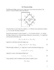
40, 41] show the position of cells on the Young’s modulus<br />
chart, Figure 3. One can see that the cells are <strong>in</strong>deed softer<br />
than other materials typically <strong>in</strong> use <strong>in</strong> biology. There is considerable<br />
variation of rigidity with<strong>in</strong> cells of different type.<br />
Epithelial cells seem to be the softest ones. Edge of young<br />
epithelial cell can have a Young’s modulus of ∼0.2 kPa [133].<br />
Platelets are the toughest with Young’s modulus as high as<br />
hundreds of kilopascals.<br />
When measur<strong>in</strong>g cell mechanics, it is of paramount<br />
importance to do multiple measurements to ga<strong>in</strong> enough<br />
statistical knowledge. It is not a trivial statement for many<br />
physicists and chemists. Intr<strong>in</strong>sic variability of biological
<strong>Atomic</strong> <strong>Force</strong> <strong>Microscopy</strong> <strong>in</strong> <strong>Cancer</strong> <strong>Cell</strong> <strong>Research</strong> 7<br />
Figure 3. The Young’s moduli of different materials. The diagram<br />
shows a spectrum from very hard to very soft:steel > bone > collagen ><br />
prote<strong>in</strong> crystal > gelat<strong>in</strong>, rubber > cells. Note a considerable variation<br />
of rigidity even with<strong>in</strong> cells. Repr<strong>in</strong>ted with permission from [1], J. L.<br />
Alonso and W. H. Goldmann, Life Sciences 72, 2553 (2003). © 2003.<br />
forms is considerably higher than typically known <strong>in</strong> either<br />
physics or chemistry. Furthermore even with<strong>in</strong> one cell there<br />
are different areas of rigidity, which can be different by<br />
orders of magnitude [25, 133, 140]. For example, as was<br />
shown <strong>in</strong> Berdyyeva et al. [133], the difference <strong>in</strong> rigidity<br />
at the cytoplasmic area and cell edge can have more than<br />
two orders of magnitude. The next factor of uncerta<strong>in</strong>ty can<br />
be the cell age and its mitosis stage. It was demonstrated<br />
[141] on normal rat kidney (NRK) fibroblasts (ATCC) cells<br />
that the Young’s modulus of the middle (between nuclei)<br />
of divid<strong>in</strong>g cell changes from ∼1 kPa (dur<strong>in</strong>g <strong>in</strong>terphase)<br />
to ∼10 kPa (dur<strong>in</strong>g cytok<strong>in</strong>esis). Results of Berdyyeva et al.<br />
[133] show that a similar change <strong>in</strong> rigidity (about 10 times)<br />
can be observed on epithelial cells while ag<strong>in</strong>g <strong>in</strong> vitro.<br />
F<strong>in</strong>ally, the Young’s modulus can depend on the depth of<br />
probe penetration. Without the special analysis and model<strong>in</strong>g<br />
of cells as a multilayered shape, one obviously can speak<br />
about the effective Young’s modulus of the cell only. All of<br />
these problems demonstrate that one has to be very careful<br />
<strong>in</strong> choos<strong>in</strong>g the appropriate cell model to study cell rigidity.<br />
These and other issues will be discussed later.<br />
3.2. How to Measure Rigidity of <strong>Cell</strong>s with<br />
AFM: Experimental Steps<br />
<strong>Cell</strong> rigidity can be measured us<strong>in</strong>g force mode, which<br />
was described <strong>in</strong> the Introduction. As a result of measurements<br />
<strong>in</strong> the force mode, one gets a force curve (force vs.<br />
z-position of the sample). An example of two such measurements<br />
done on two surfaces of different rigidities is shown <strong>in</strong><br />
Figure 4 (only approach<strong>in</strong>g curves are shown). After contact,<br />
the AFM tip touches the surface and the cantilever deflects<br />
up. The correspond<strong>in</strong>g force, plotted <strong>in</strong> Figure 4, is equal to<br />
the cantilever deflection multiplied by the spr<strong>in</strong>g constant of<br />
the cantilever. If you have two different surfaces, one softer<br />
and one harder, there is larger deflection of the cantilever<br />
on harder surface. This is because the harder surface pushes<br />
the cantilever up stronger, while the softer surface lets the<br />
cantilever penetrate deep <strong>in</strong>side. Thus, measur<strong>in</strong>g the slope<br />
of the force curve after the contact (region of constant compliance),<br />
one can get <strong>in</strong>formation about surface rigidity.<br />
Us<strong>in</strong>g these force curves (sometime called <strong>in</strong>dentation<br />
curves), one can easily calculate the stiffness, which is def<strong>in</strong>ed<br />
as a derivative of force F with respect to penetration p<br />
(<strong>in</strong>dentation), dF/dp. To calculate penetration, one can use<br />
Figure 4. <strong>Force</strong>–distance curves for two materials of different rigidity.<br />
Only approach<strong>in</strong>g curves are shown.<br />
a simple formula p = z − d, which can be obta<strong>in</strong>ed from<br />
straightforward geometrical considerations. Here d is deflection<br />
of the cantilever (positive when it deflects up), and z<br />
is the vertical position of the sample (and is equal to zero<br />
at the moment of the tip-sample contact). While stiffness is<br />
a rather well-def<strong>in</strong>ed characteristic of surfaces, it is not a<br />
clear characteristic of materials. Stiffness depends not only<br />
on Young’s modulus of rigidity (which is a material characteristic),<br />
but also on the geometry of the tip-surface contact.<br />
Therefore, to be able to compare different materials,<br />
one needs to deal with Young’s modulus of rigidity, which is<br />
<strong>in</strong>dependent of the tip geometry. How to calculate Young’s<br />
modulus will be described <strong>in</strong> the next sections. Below we<br />
will describe the major experimental steps needed to measure<br />
mechanics of both normal and cancer cells. Because<br />
there are too many experimental approaches <strong>in</strong> study<strong>in</strong>g<br />
cell mechanics, description of such steps is very important.<br />
Eventually it may be promoted as a sort of protocol, the<br />
researchers able to compare the mechanics of a large variety<br />
of different cells.<br />
3.2.1. <strong>Cell</strong> Culture Preparation<br />
Before imag<strong>in</strong>g, cells should be attached to some rigid substrate,<br />
usually either a slide or the bottom of a Petri dish.<br />
It is recommended to use specially coated dishes or slides<br />
to facilitate adhesion. Such Petri dishes or slides are available<br />
commercially, or can be prepared by coat<strong>in</strong>g with various<br />
molecules that have suitable am<strong>in</strong>o groups, see, e.g.,<br />
Sagvolden et al. [43]. After that the slide/dish has to be<br />
mounted on the AFM stage, for example with doublestick<br />
tape. Size of the Petri dishes is also important to<br />
have convenient measurements. Work<strong>in</strong>g with larger Petri<br />
dishes requires the removal of a part the dish side, which is<br />
extremely <strong>in</strong>convenient.<br />
Right before plac<strong>in</strong>g the cells <strong>in</strong> the AFM for analysis,<br />
the culture medium should be replaced by a balanced buffer<br />
which does not conta<strong>in</strong> prote<strong>in</strong>s. Phosphate-buffered sal<strong>in</strong>e<br />
(PBS) or Hank’s buffered sal<strong>in</strong>e solution (HBSS) are good<br />
choices. Work<strong>in</strong>g at room temperature, the cells are typically<br />
viable <strong>in</strong> these buffers for a few hours. For example,<br />
we found that human epithelial cells can survive at least
8 <strong>Atomic</strong> <strong>Force</strong> <strong>Microscopy</strong> <strong>in</strong> <strong>Cancer</strong> <strong>Cell</strong> <strong>Research</strong><br />
3–4 hours <strong>in</strong> HBSS and at least 2–3 hours <strong>in</strong> PBS solution.<br />
Obviously this time will decrease if work<strong>in</strong>g at elevated<br />
temperatures.<br />
3.2.2. AFM Probe Preparation<br />
To measure the rigidity of such materials, virtually any regular<br />
AFM cantilevers can be used. Spr<strong>in</strong>g constants can<br />
be <strong>in</strong> the broad range of 0.001–100 N m−1 . The optimum<br />
spr<strong>in</strong>g constant should be approximately equal to the effective<br />
spr<strong>in</strong>g constant, or stiffness, of the surface. Because cells<br />
are soft, a possible AFM tip penetration can be quite large.<br />
The part of the tip which is <strong>in</strong> contact with the cell will<br />
also be large. Consequently, that part of the tip shape has<br />
to be well-def<strong>in</strong>ed. A standard AFM tip is rather sharp. Tip<br />
penetration is typically much larger than the radius of the<br />
tip apex. Therefore one needs to know the tip geometry <strong>in</strong><br />
larger scale. A regular AFM tip has a cone geometry on the<br />
larger scale. Such tips have been widely used [19, 20, 26–29,<br />
40, 134, 142] to study cells. The major problem with such tips<br />
is that they <strong>in</strong>duce too large a stress <strong>in</strong> the vic<strong>in</strong>ity of the tip<br />
apex [143, 144]. Such a large stress can lead to nonl<strong>in</strong>earity<br />
<strong>in</strong> the material response. The second major issue with sharp<br />
AFM tips is the relatively small area of contact. <strong>Cell</strong>s can<br />
have rather <strong>in</strong>homogeneous surfaces. Structural cytoskeleton<br />
fibers can sit directly underneath the cell surface. When<br />
the area of contact is small, the tip can be either right above<br />
the fibers or between the fibers. As a result, measured rigidities<br />
can vary broadly. To get robust statistics, one needs<br />
to do too many force measurements. At the same time,<br />
one has limited time <strong>in</strong> the experiment to ma<strong>in</strong>ta<strong>in</strong> viability<br />
of cells.<br />
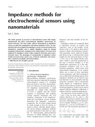
The solution to the above problems is <strong>in</strong> us<strong>in</strong>g welldef<strong>in</strong>ed<br />
dull tips. Such tips can be made by glu<strong>in</strong>g a colloidal<br />
spherical particle to the AFM cantilever [133, 144–147].<br />
Figure 5 shows an example of a V-shaped standard AFM<br />
cantilever with a 5-m-diameter silica ball glued with epoxy<br />
res<strong>in</strong>. One can clearly see a big difference <strong>in</strong> the area of<br />
contacts of a regular pyramidal tip and the silica ball. In<br />
general it is easier to use special tipless cantilevers for the<br />
attachment of such large colloidal probes.<br />
The larger area of probe-cell contact results <strong>in</strong> averag<strong>in</strong>g<br />
local variation <strong>in</strong> rigidity compared to that measured<br />
with a regular sharp probe. On some type of epithelial sk<strong>in</strong><br />
cells, we measured the standard deviation <strong>in</strong> the distribution<br />
of Young’s modulus up to 200–300% when measur<strong>in</strong>g with<br />
regular <strong>in</strong>tegrated pyramidal silicon nitride tips (DNP-S by<br />
Veeco/DI Inc.). That spread was reduced almost by an order<br />
of magnitude when us<strong>in</strong>g silica ball tips. Although for some<br />
other types of cells this difference is not that pronounced.<br />
Overall reduction of the spread is greatly helpful for atta<strong>in</strong><strong>in</strong>g<br />
robust statistics of measurements.<br />
There is a couple of other advantages of us<strong>in</strong>g colloidal<br />
probe particles. Due to the low rigidity at th<strong>in</strong> edge of some<br />
cells, it would be very hard, if not impossible, to make measurements<br />
with a sharp AFM tip. The sharp tip simply penetrates<br />
the th<strong>in</strong> areas of the cell and shows even higher<br />
rigidity due to touch<strong>in</strong>g the rigid substrate. Us<strong>in</strong>g colloidal<br />
probe particles such th<strong>in</strong> areas can easily be measured.<br />
Figure 5. An example of a V-shaped standard AFM cantilever (apex<br />
diameter, 50 nm) with a 5-m-diameter silica ball glued with epoxy<br />
res<strong>in</strong>. Repr<strong>in</strong>ted with permission from [133], T. K. Berdyyeva et al.,<br />
Phys. Med. Biol. 50, 81 (2005). © 2005.<br />
3.2.3. Tip Geometryand the Cantilever<br />
Spr<strong>in</strong>g Constant<br />
To extract the <strong>in</strong>formation about the Young’s modulus of<br />
rigidity from measured data, one needs to know the cantilever<br />
spr<strong>in</strong>g constant and exact tip geometry. The radius of<br />
the probe and its cleanl<strong>in</strong>ess can be tested by scann<strong>in</strong>g the<br />
reverse grid (TGT01, Micromash, Inc., Estonia), and sometimes<br />
with SEM. TGT01 grid is a set of very sharp silicon tips<br />
which have radii of the apex less than 5–10 nm, Figure 6, left.<br />
Scann<strong>in</strong>g over such tips with the large colloidal probe results<br />
<strong>in</strong> a k<strong>in</strong>d of “<strong>in</strong>versed” image of the probe. Effectively, the<br />
sharp AFM imag<strong>in</strong>g tip is now attached to the surface, and<br />
the colloidal probe plays the role of a sample. The image of<br />
colloidal probe is produced by each silicon tips. An example<br />
ofa5m silica ball probe scanned over the sharp silicon<br />
needles, the reverse grid is shown <strong>in</strong> Figure 6, right image.<br />
Process<strong>in</strong>g this data with any software that allows non-l<strong>in</strong>ear<br />
Figure 6. An SEM image of TGT01 grid (left image; Repr<strong>in</strong>ted with<br />
permission from MicroMash, Inc., Estonia). Reverse grid image of a<br />
5-m silica ball attached to AFM cantilever.
<strong>Atomic</strong> <strong>Force</strong> <strong>Microscopy</strong> <strong>in</strong> <strong>Cancer</strong> <strong>Cell</strong> <strong>Research</strong> 9<br />
curve fitt<strong>in</strong>g, one can f<strong>in</strong>d the radius of AFM probe attached<br />
to the cantilever.<br />
The cantilever spr<strong>in</strong>g constant can be found us<strong>in</strong>g different<br />
procedures described <strong>in</strong> a host of literature [147–<br />
153]. Us<strong>in</strong>g V-shaped cantilevers from Veeco/DI, one can<br />
utilize a built-<strong>in</strong> option of the Nanoscope software to f<strong>in</strong>d<br />
the spr<strong>in</strong>g constant of the cantilever. The newer versions of<br />
the Nanoscopes software conta<strong>in</strong> implementation of another<br />
method which is based on thermal fluctuation analysis. That<br />
method is more cantilever-shape <strong>in</strong>dependent, but can be<br />
applied only to sufficiently soft cantilevers.<br />
3.2.4. Cantilever SensitivityCalibration<br />
This is the first necessary step before mak<strong>in</strong>g actual measurements.<br />
Deflection of the cantilever is detected by either<br />
a photodiode or a piezosensor (piezolever). Both detectors<br />
give read<strong>in</strong>gs <strong>in</strong> electrical units, i.e., Volts. However, for the<br />
force measurements one needs to get the cantilever deflection<br />
<strong>in</strong> the units of length, i.e., meters (or nanometers). The<br />
coefficient that converts Volts <strong>in</strong>to meters has to be measured<br />
each time after align<strong>in</strong>g the laser on the cantilever<br />
(or chang<strong>in</strong>g the piezolever). F<strong>in</strong>d<strong>in</strong>g such a coefficient is<br />
called sensitivity calibration of the cantilever. Specific technical<br />
realization of such calibration can depend on AFM<br />
manufactures. However <strong>in</strong> all cases, this can technically be<br />
done by record<strong>in</strong>g a force curve on a sample that can be<br />
treated as absolutely rigid material. In that case, both the tip<br />
and simple surface move together after the contact. Because<br />
the shift of the sample (<strong>in</strong> the units of length, nm) is known,<br />
one has to equalize it to the change <strong>in</strong> the voltage of photodiode<br />
(<strong>in</strong> the units of voltage, Volts).<br />
It is best to perform the calibration prior to perform<strong>in</strong>g<br />
an experiment because the cantilever may become damaged<br />
dur<strong>in</strong>g the experiment. If this occurs, then one can no longer<br />
do the calibration and the recorded force data can be lost.<br />
Secondly, the obta<strong>in</strong>ed spr<strong>in</strong>g constant can reveal possibly<br />
damaged cantilever. In the later case, one would observe<br />
noticeably less spr<strong>in</strong>g constant than its nom<strong>in</strong>al value typically<br />
given by the manufacturer.<br />
It is useful to note that the photodiodes used <strong>in</strong> AFMs<br />
are fairly l<strong>in</strong>ear with respect to the position of the laser spot.<br />
Therefore, realign<strong>in</strong>g the position on the photodiode (detector)<br />
with respect to the laser spot position does not require<br />
recalibration.<br />
3.2.5. Us<strong>in</strong>g <strong>Force</strong>–Volume Mode<br />
Hav<strong>in</strong>g calibrated the cantilever, one can start collect<strong>in</strong>g<br />
force data. The tip can be located above the cell with the<br />
help of any optical system. For example, one AFM has a<br />
built-<strong>in</strong> optical video microscope, which allows observation<br />
of areas from 150 m × 110 m to675m × 510 m, with<br />
1.5 m resolution. Simultaneous position of the tip can be<br />
done with lateral accuracy of ∼10 m. Before go<strong>in</strong>g to the<br />
force–volume mode, a s<strong>in</strong>gle good force curve should first<br />
be obta<strong>in</strong>ed. To get such a curve, one should use the force<br />
mode. The goal of this step is to optimize the variety of<br />
parameters of the force mode such as the ramp size and<br />
the trigger level (see above). After optimiz<strong>in</strong>g the parameters<br />
and record<strong>in</strong>g a good force curve, one should proceed<br />
to the force–volume mode to collect large amount of the<br />
force data.<br />
The important parameters <strong>in</strong> the force–volume mode are<br />
the number of pixels on the cell surface <strong>in</strong> which the force<br />
<strong>in</strong>formation will be recorded, and the speed of oscillation of<br />
the AFM tip. Typically, the choice of the oscillation speed<br />
is a compromise between the duration of the data collection<br />
and work<strong>in</strong>g <strong>in</strong> the regime where the viscoelastic effects are<br />
not very pronounced. The number of pixels should be sufficient<br />
to dist<strong>in</strong>guish the variability of stiffness over the cell<br />
surface, as well as topography of the surface itself.<br />
One note should be mentioned about a possible range<br />
of the ramp size. It is restricted by the maximum range of<br />
the scanner <strong>in</strong> the vertical direction. If one uses the relative<br />
trigger mode (recommended option for the safety of the<br />
cantilever), the maximum size is only the half of the maximum<br />
scanner range. This creates a problem for a majority<br />
of AFM scanners because the cells have heights which<br />
are normally quite large. To avoid this problem, the area<br />
of the whole cell can be split <strong>in</strong>to a series of small areas;<br />
each of those has suitable height variation. The measurements<br />
should be done on each of these small areas. Alternatively,<br />
a new scanner with a larger vertical range is needed.<br />
Fortunately, such scanners are commercially available. To<br />
be sure that the scanner is free of possible nonl<strong>in</strong>earities<br />
at such a large scale, the closed-loop type of scanner is<br />
recommended.<br />
3.2.6. Control Experiments<br />
The purpose of such experiments is to exclude any changes<br />
<strong>in</strong> rigidity which could be artifacts of imag<strong>in</strong>g or culture<br />
preparation. There can be a number of such experiments.<br />
Section 3.5.3 below describes different sources of uncerta<strong>in</strong>ty<br />
and possible alteration of cell rigidity due to either<br />
culture preparation or AFM technique itself. The control<br />
experiments that have to be done depend on the cell type.<br />
Below we describe an example of such a control experiment<br />
performed <strong>in</strong> the case of human sk<strong>in</strong> epithelial cells.<br />
Pok<strong>in</strong>g a cell with the AFM tip dur<strong>in</strong>g measurements<br />
can potentially cause <strong>in</strong>ternal changes <strong>in</strong> the cell. There is<br />
some evidence [142] that the tip can cause alteration of<br />
the cytoskeleton. Different types of cells can have different<br />
responses to the action of the AFM probe. Therefore,<br />
it is logical to conduct a controlled experiment, cont<strong>in</strong>uously<br />
measur<strong>in</strong>g mechanical properties of the cell dur<strong>in</strong>g<br />
scann<strong>in</strong>g <strong>in</strong> the force–volume mode. For example, as was<br />
shown elsewhere [133], the AFM probe cont<strong>in</strong>uously measured<br />
(<strong>in</strong> force–volume mode) a cell along the same l<strong>in</strong>e<br />
at 32 po<strong>in</strong>ts for about two hours. No significant change <strong>in</strong><br />
rigidity was detected. It should be noted that small alterations<br />
<strong>in</strong> Young’s modulus may be a result of gentle force–<br />
volume scann<strong>in</strong>g. This is not necessarily the case for the<br />
contact or Tapp<strong>in</strong>g imag<strong>in</strong>g modes of scann<strong>in</strong>g, where both<br />
relatively large vertical and lateral drag forces are applied to<br />
the cell.<br />
3.3. How to Measure <strong>Cell</strong> Rigidity with AFM:<br />
Young’s Modulus Calculations<br />
After the collection of data, it should be processed. In<br />
this section we consider different models to extract Young’s
10 <strong>Atomic</strong> <strong>Force</strong> <strong>Microscopy</strong> <strong>in</strong> <strong>Cancer</strong> <strong>Cell</strong> <strong>Research</strong><br />
modulus of rigidity from the force curves measured as<br />
described above. To f<strong>in</strong>d Young’s modulus, one needs to<br />
know the tip geometry and structure of the sample. The<br />
tip geometry can be found as described above. However,<br />
the structure of the sample is too complicated to be treated<br />
without any assumptions. Here we will assume that the cell<br />
is a homogeneous, isotropic medium. Obviously this is an<br />
approximation. There is a plethora of literature show<strong>in</strong>g that<br />
such an approximation is plausible [19, 20, 26–29, 40, 134,<br />
136–139]. We will demonstrate this <strong>in</strong> more detail later <strong>in</strong><br />
this section.<br />
Configuration of a spherical probe over a flat homogeneous<br />
surface is described by the Hertz–Sneddon model<br />
[107, 154, 155]. This model was developed for either a spherical<br />
probe of radius R or a parabolic tip over a plane surface.<br />
In the case of a parabolic tip described by equation<br />
Z = b · X 2 , the effective radius R can be found as 1/2b. In<br />
this model, the Young’s modulus E is given by<br />
E = 3 1 − <br />
4<br />
2 dF<br />
√<br />
R dp3/2 (1)<br />
<br />
where F is the load force, R is the radius of the ball, p is the<br />
probe penetration <strong>in</strong>to the cell. The Poisson ratio of the<br />
cells is unknown. For the majority of biological materials,<br />
= 05. Nonetheless, we will treat the Poisson ratio to be<br />
unknown. To remove this uncerta<strong>in</strong>ty, we will speak about<br />
an “apparent” Young’s modulus, to be def<strong>in</strong>ed as follows<br />
Eapp = E<br />
1 − 2 (2)<br />
In the derivation of Eq. (1) it was assumed that the rigidity<br />
of the probe is much higher than the rigidity of the sample.<br />
This is generally true for the majority of AFM probes. The<br />
Hertz–Sneddon model has also two additional assumptions.<br />
The first one is that the probe penetration <strong>in</strong>to the sample<br />
should be much smaller than the radius of the probe. This<br />
can easily be controlled. The second assumption is about<br />
the lack of adhesion between the probe and sample surface.<br />
Look<strong>in</strong>g at the force curves, one can easily identify the<br />
adhesion (Fadd <strong>in</strong> Fig. 2). If the adhesion is high, one has<br />
to use another model, the so-called JKR (Johnson–Kandall–<br />
Roberts) model [156–161] to f<strong>in</strong>d the Young’s modulus. The<br />
material of the probe can be chosen, or altered to ensure low<br />
adhesion. Typically the adhesion between an AFM probe<br />
(for example, a clean silica sphere) and a cell is low. Therefore,<br />
we will not describe the JKR model here, referr<strong>in</strong>g the<br />
reader to the orig<strong>in</strong>al literature [156–161].<br />
The majority of standard AFM cantilevers have a conical<br />
shape. It is useful to present a result of application of the<br />
Hertz–Sneddon model to a conical probe. For a conical tip<br />
with a semivertical (open<strong>in</strong>g) angle , the apparent Young’s<br />
modulus can be given by the follow<strong>in</strong>g formula<br />
Eapp = 1 dF<br />
tan <br />
2 dp2 (3)<br />
<br />
Let us show an example of the application of the Hertz–<br />
Sneddon model to an epithelial cell. It is well known that<br />
the cell is a very complicated object from a structural<br />
po<strong>in</strong>t of view. Nevertheless as we have already mentioned,<br />
it is surpris<strong>in</strong>gly well described by the approximation of<br />
a homogeneous medium. From the general po<strong>in</strong>t of view<br />
such an assumption is not that unexpected if we deal with<br />
small deformations. However, for larger deformations this<br />
assumption is obviously broken. Accord<strong>in</strong>g to Eq. (1), a plot<br />
of the load force versus the probe penetration to the 3/2th<br />
power must be a straight l<strong>in</strong>e. Figure 7 demonstrates the<br />
results of process<strong>in</strong>g about 30 force curves averaged over<br />
an edge of epithelial cell [133]. (The approach force curves<br />
were used here. A 5-m silica ball was used as a colloidal<br />
probe.) One can see <strong>in</strong> Figure 7 that the Hertz–Sneddon<br />
model is a good approximation until p 3/2 = 4000 nm 3/2 ,<br />
which corresponds to a penetration of ∼250 nm. It is <strong>in</strong>terest<strong>in</strong>g<br />
to note that for sufficiently large penetrations, the<br />
Hertz–Sneddon model starts work<strong>in</strong>g aga<strong>in</strong>. One can see<br />
<strong>in</strong> Figure 7 that the force-p 3/2 curve can aga<strong>in</strong> be approximated<br />
by a straight l<strong>in</strong>e after a penetration of approximately<br />
500 nm. This is yet to be understood.<br />
3.4. Mechanics of <strong>Cancer</strong> <strong>Cell</strong>s: Results<br />
The results we discuss below are summarized <strong>in</strong> Table 1 <strong>in</strong><br />
historical order. One of the first measurements on a cancer<br />
cell l<strong>in</strong>e was done on human lung carc<strong>in</strong>oma cells [134].<br />
It showed quite a variation <strong>in</strong> the measured Young’s modulus,<br />
13–150 kPa, and was essentially a demonstration of<br />
the method. Such variability <strong>in</strong> the modulus is presumably<br />
a result of the few statistics collected dur<strong>in</strong>g these measurements.<br />
This is expla<strong>in</strong>ed by the fact that the authors did not<br />
use automated tools such as the force–volume mode, and<br />
had to collect <strong>in</strong>dividual force curves. A sharp AFM tip was<br />
used <strong>in</strong> this study.<br />
An <strong>in</strong>terest<strong>in</strong>g analysis of the rigidity of cancer cells<br />
(wild, and v<strong>in</strong>cul<strong>in</strong>-deficient, (5.51) mouse F9 embryonic<br />
carc<strong>in</strong>oma cells) has been done [19, 20]. The authors<br />
compared wild-type mouse F9 embryonic cells, which can<br />
Figure 7. Plot of probe penetration to the 1.5 power versus load<br />
force. Accord<strong>in</strong>g to Eq. (1), a straight l<strong>in</strong>e demonstrates constancy of<br />
the Young’s modulus, and therefore represents validity of the model.<br />
Repr<strong>in</strong>ted with permission from [133], T. K. Berdyyeva et al., Phys. Med.<br />
Biol. 50, 81 (2005). © 2005.
<strong>Atomic</strong> <strong>Force</strong> <strong>Microscopy</strong> <strong>in</strong> <strong>Cancer</strong> <strong>Cell</strong> <strong>Research</strong> 11<br />
Table 1. Summary table of measured apparent (i.e., where Poisson’s ratio = 0) Young’s moduli of cancer cells (with some normal stra<strong>in</strong>). Asterisk<br />
(∗) denotes data taken from Figure 7 of Park et al., with permission of the publisher [162].<br />
<strong>Cell</strong>:tissue type E [kPa] Note Ref.<br />
Human lung carc<strong>in</strong>oma cell 13–150 <strong>Cell</strong>s were collected from a 62-year-old <strong>in</strong>dividual.<br />
S<strong>in</strong>gle force–distance curves were used <strong>in</strong> analysis. Sharp AFM<br />
tip was used.<br />
[134]<br />
Mouse F9 embryonic carc<strong>in</strong>oma 3.8 ± 1.1 Correlation between rigidity and v<strong>in</strong>cul<strong>in</strong> deficiency was stud- [19, 20]<br />
V<strong>in</strong>cul<strong>in</strong>-deficient mouse F9 2.5 ± 1.5 ied further by v<strong>in</strong>cul<strong>in</strong> transfection. This confirmed gradual [19, 20]<br />
embryonic carc<strong>in</strong>oma (5.51)<br />
decrease of rigidity with the decrease of v<strong>in</strong>cul<strong>in</strong> expression.<br />
<strong>Force</strong>–volume mode was used. Sharp AFM tip was used.<br />
Hu609 (non-malignant ureter cells) 12.8 ± 4.8 Ureter and bladder cells are rather similar cell types. About [29]<br />
(normal cell) 20 cells of each type were measured. A sort of force–volume<br />
mode was used. Sharp AFM tip was used.<br />
HCV29 (non-malignant bladder urothelium) 10.0 ± 4.6<br />
(normal cell)<br />
T24 (bladder transitional cell carc<strong>in</strong>oma) 1.0 ± 0.5<br />
BC3726 (HCV29 cells transfected with<br />
v-ras oncogene)<br />
1.4 ± 0.5<br />
Hu456 (bladder transitional cell carc<strong>in</strong>oma) 0.4 ± 0.3<br />
Fibroblast BALB 3T3 1.3 ± 1.0∗ Average over the cell values are shown. Only a few force curves [162]<br />
(normal cell) per cell were collected.<br />
Fibroblast:SV-T2 0.6 ± 0.5∗ Fibroblast:H-ras 0.5 ± 0.5∗ attach and spread well on extracellular matrix, and v<strong>in</strong>cul<strong>in</strong>deficient<br />
(5.51) cells, which conta<strong>in</strong> no detectable v<strong>in</strong>cul<strong>in</strong><br />
prote<strong>in</strong> and spread poorly on substrates. In these measurements<br />
the researchers used the force–volume mode to<br />
collect enough statistics. It allowed them to calculate the<br />
standard deviation of the Young’s modulus distribution.<br />
Young’s modulus of 3.8 ± 1.1 kPa and 2.5 ± 1.5 kPa, was calculated<br />
for wild-type and 5.51 cells, respectively. It should<br />
be noted that <strong>in</strong> all these calculations the standard deviation<br />
<strong>in</strong> the distribution comes not from the error of measurements<br />
but rather from the <strong>in</strong>tr<strong>in</strong>sic variability of the modulus<br />
distribution over different cells as well as for a s<strong>in</strong>gle<br />
cell surface. Despite the fact that the difference <strong>in</strong> rigidity<br />
was only ∼20–25%, it was further corroborated by study<strong>in</strong>g<br />
v<strong>in</strong>cul<strong>in</strong>-transfected cells. In those cells the amount of stress<br />
fiber versus the F-act<strong>in</strong> mesh was different, and the expected<br />
gradual change of rigidity was detected. A sharp AFM tip<br />
was used <strong>in</strong> this study.<br />
It is def<strong>in</strong>itely of great <strong>in</strong>terest to compare the mechanics<br />
of normal and malignant cells of the same type. The first<br />
comparative study of the mechanics of tumor and normal<br />
cells was reported <strong>in</strong> 1999 [27, 29]. <strong>Cell</strong>s of similar types<br />
were studied:Hu609 (non-malignant ureter cells), Hu456<br />
(bladder transitional cell carc<strong>in</strong>oma cell), HCV29 (nonmalignant<br />
bladder urothelium cell), BC3726 (HCV29 cells<br />
transfected with v-ras oncogene), and T24 (bladder transitional<br />
cell carc<strong>in</strong>oma, ATCC HTB4). In that careful study,<br />
the researchers collected enough data to derive statistically<br />
sound results. The results for Young’s modulus of these cells<br />
are shown <strong>in</strong> Table 1. One can see rather substantial differences<br />
<strong>in</strong> rigidity among the various cell types. <strong>Cancer</strong><br />
cells were reported to be softer than normal cells, by up to<br />
one order of magnitude. Moreover, some nonl<strong>in</strong>earity was<br />
detected for normal cells:Young’s modulus for the normal<br />
stra<strong>in</strong> Hu609 calculated for lower load forces (up to 2 nN)<br />
was 15.2 ± 4.7 kPa, versus 12.9 ± 4.8 kPa obta<strong>in</strong>ed for large<br />
forces (5–10 nN). Young’s moduli calculated for cancerous<br />
cell l<strong>in</strong>es were almost <strong>in</strong>dependent of the load. Furthermore,<br />
for small probe penetration depths (lower than 100 nm),<br />
when the <strong>in</strong>fluence of the membrane was the highest, the<br />
difference between normal and cancerous cells was not visible.<br />
The reported method could not dist<strong>in</strong>guish between<br />
normal and cancerous cell membrane mechanics, while the<br />
difference between normal and cancerous cells was rather<br />
clear with the <strong>in</strong>crease of the probe penetration depth.<br />
Recently, local rigidity differences between normal fibroblasts<br />
(BALB 3T3) and cancer cells (SV-T2 and H-rastransformed<br />
fibroblasts) were <strong>in</strong>vestigated [162]. Although<br />
that work was focused on the correlation between motility<br />
and viscoelasticity of cells, a clear decrease of the<br />
Young’s moduli of normal and cancer cells was observed.<br />
The Young’s moduli were measured at about three different<br />
po<strong>in</strong>ts on each fibroblast. Specifically, 38 po<strong>in</strong>ts from<br />
13 BALB 3T3 fibroblasts, 29 po<strong>in</strong>ts from 10 SV-T2 fibroblasts,<br />
and 18 po<strong>in</strong>ts from 8 H-ras-transformed fibroblasts.<br />
Averaged moduli (over three po<strong>in</strong>ts per cell) are shown<br />
<strong>in</strong> Table 1. There is also a significant difference <strong>in</strong> the<br />
elastic constants of lamellipodia (lead<strong>in</strong>g edge of the cell)<br />
between normal (1.01 ± 0.40 kPa) and malignantly transformed<br />
fibroblasts whereas there is no significant difference<br />
between SV-T2 (0.48 ± 0.51 kPa) and H-ras-transformed<br />
fibroblasts (0.42 ± 0.35 kPa). Normal fibroblasts displayed a<br />
much wider distribution of Young’s modulus (0.34–4.95 kPa)<br />
than the malignantly transformed fibroblasts. There was no<br />
occurrence of elastic constants exceed<strong>in</strong>g 3.0 kPa for the<br />
malignantly transformed fibroblasts.<br />
It should be noted that a def<strong>in</strong>ite difference <strong>in</strong> Young’s<br />
modulus at different po<strong>in</strong>ts on the cell was observed. However,<br />
not enough statistics were taken. It is <strong>in</strong>terest<strong>in</strong>g to<br />
note that the authors use not only the Hertz model to calculate<br />
Young’s modulus. More complicated models [31, 163,<br />
164], which take <strong>in</strong>to account a possible <strong>in</strong>fluence of the<br />
substrate were utilized. The Young’s modulus <strong>in</strong> the thicker<br />
cellular regions closer to the cell body (cytoplasmic area),
12 <strong>Atomic</strong> <strong>Force</strong> <strong>Microscopy</strong> <strong>in</strong> <strong>Cancer</strong> <strong>Cell</strong> <strong>Research</strong><br />
was successfully derived us<strong>in</strong>g the Hertz model. The measure<br />
of success here was def<strong>in</strong>ed as <strong>in</strong>dependence of Young’s<br />
modulus from the penetration depth. Th<strong>in</strong>ner lamellipodia<br />
areas were analyzed with the Tu model or the Chen model<br />
[163, 164] due to the substrate effect (which was seen as a<br />
strong dependence of the Young’s modulus on the penetration<br />
depth).<br />
3.5. Discussion<br />
3.5.1. General Analysis of the<br />
Studied Mechanics<br />
When approach<strong>in</strong>g the cell surface, the AFM probe encounters<br />
first the layer of glycocalyx (polysaccharide molecules<br />
cover<strong>in</strong>g cytoplasmic membrane), then the cell membrane<br />
re<strong>in</strong>forced with a mesh of F-act<strong>in</strong>, and f<strong>in</strong>ally, the deeper cell<br />
body. Mechanical differences between normal and cancerous<br />
cells <strong>in</strong> all of these layers can contribute to the measured<br />
Young’s modulus with the AFM method. Let us analyze<br />
the exist<strong>in</strong>g data to understand possible <strong>in</strong>fluences of these<br />
layers.<br />
Note that a sharp AFM tip was used <strong>in</strong> the first measurements<br />
[19, 20, 27, 29, 134]. It is highly unlikely that<br />
the layer of glycocalyx could be detected with such a sharp<br />
tip. What about the next membrane layer? As has been<br />
noted [29], a sharp AFM tip could not dist<strong>in</strong>guish between<br />
normal and cancerous cell membrane mechanics, while the<br />
difference between normal and cancerous cells was rather<br />
clear with the <strong>in</strong>crease of the probe penetration depth. This<br />
may mean that there are <strong>in</strong>deed no detectable differences<br />
between membranes <strong>in</strong> cancer and normal cells, or alternatively,<br />
the sharp AFM tip is not capable of detect<strong>in</strong>g such<br />
differences. The difference <strong>in</strong> cortical layer of F-act<strong>in</strong> is<br />
expected for normal and cancer cells [168, 169]. Therefore it<br />
is probable that the sharp AFM tip is simply not capable of<br />
detect<strong>in</strong>g the difference. This seems to be <strong>in</strong> agreement with<br />
the conclusion of previous works [19, 20]. In those works<br />
the authors noted that <strong>in</strong> wild-type cells, F-act<strong>in</strong> is organized<br />
<strong>in</strong>to bundles (stress fibers) which term<strong>in</strong>ate at focal contacts,<br />
whereas v<strong>in</strong>cul<strong>in</strong>-deficient cells show no act<strong>in</strong> stress fibers,<br />
and <strong>in</strong>stead F-act<strong>in</strong> is concentrated under the plasma membrane.<br />
Based on that, they concluded that rigidity was more<br />
<strong>in</strong>fluenced by stress fibers (located more deeply <strong>in</strong> the cell<br />
body) rather than F-act<strong>in</strong> mesh (located immediately under<br />
the plasma membrane).<br />
A much larger polystyrene ball of 1–4 m (1000–4000 nm)<br />
<strong>in</strong> diameter (compared with a diameter of 10–100 nm1 for the sharp AFM probe) was used as an AFM probe<br />
<strong>in</strong> recently reported measurements [162]. As one can see<br />
from Table 1, differences <strong>in</strong> Young’s modulus were clearly<br />
detected. However, the differences <strong>in</strong> the modulus values<br />
was nearly the same as the variation with<strong>in</strong> the cancerous<br />
cells reported by Lekka et al. [29]. Nevertheless, the analysis<br />
by Park et al. [162] was done <strong>in</strong> a more precise way. To<br />
measure an order of magnitude difference <strong>in</strong> Lekka et al.<br />
1 It should be noted that the sharp AFM tips used <strong>in</strong> these studies<br />
had <strong>in</strong>deed pyramidal shape, which can be described by a cone model.<br />
The effective contact area of such tip is higher than one assumed from<br />
the curvature radius of the apex.<br />
the authors did not need too precise a knowledge of the<br />
cantilever spr<strong>in</strong>g constant and the tip radius. Whereas <strong>in</strong><br />
Park et al. the spr<strong>in</strong>g constant was not assumed but measured<br />
to a high precision (∼5%), and the tip radius as well<br />
(us<strong>in</strong>g the methods described here <strong>in</strong> Section 3.2.3). The<br />
high variability of the modulus has still to be understood.<br />
A somewhat low number of statistics with<strong>in</strong> each cell (three<br />
po<strong>in</strong>ts per cell) does not allow conclud<strong>in</strong>g it is <strong>in</strong>tr<strong>in</strong>sic variation<br />
of Young’s modulus.<br />
It is <strong>in</strong>terest<strong>in</strong>g to note one more potential source of variability<br />
can be hidden <strong>in</strong> a rather complicated analysis of the<br />
force curve done <strong>in</strong> Park et al. [162]. The authors found that<br />
the force curves measured on thick regions of the cell can be<br />
well-described with the Hertz model, i.e., the Young’s modulus<br />
derived with<strong>in</strong> such a model does vary directly with the<br />
probe penetration. However, if the force curves are taken<br />
near the cell edge, the Hertz model does not give a constant<br />
modulus. This was plausibly <strong>in</strong>terpreted as <strong>in</strong>fluence by<br />
the cell substrate, and consequently, processed us<strong>in</strong>g multilayered<br />
models [163, 164] treat<strong>in</strong>g cells as a layer on a substrate.<br />
The substrate can be either softer (a gap between a<br />
Petri dish and the cell) or harder (the cell on the Petri dish).<br />
The major assumption here is that the whole cell was treated<br />
as a homogeneous medium with the same Young’s modulus.<br />
While it is def<strong>in</strong>itely a plausible assumption, <strong>in</strong> particular,<br />
for the th<strong>in</strong> cell, it “unifies” all cell layers by treat<strong>in</strong>g the cell<br />
body as homogeneous and isotopic medium. This may br<strong>in</strong>g<br />
additional variation <strong>in</strong> such an overall cell rigidity.<br />
Can we make the conclusion that a large spherical AFM<br />
probe is capable of detect<strong>in</strong>g cell membrane/cortical layer?<br />
Presumably the answer is yes. For the example of epithelial<br />
cells, a very good def<strong>in</strong>ition of Young’s modulus derived<br />
from the Hertz model was observed <strong>in</strong> Berdyyeva et al. [133],<br />
<strong>in</strong> which a 5-m silica colloidal probe was used. This def<strong>in</strong>ition<br />
is shown <strong>in</strong> Figure 7. One can see good def<strong>in</strong>ition<br />
of the Young’s modulus for small penetrations (as well as<br />
for large penetrations). As was found <strong>in</strong> Berdyyeva et al.,<br />
the measured Young’s modulus for small penetrations is well<br />
correlated with the surface density of fibers <strong>in</strong> the cortical<br />
layer, but less correlated with the total amount of cytoskeletal<br />
fibers. This supports our conclusion that the first part of<br />
the force curve recorded with AFM colloidal probe is determ<strong>in</strong>ed<br />
by cortical layer of cytoplasmic membrane.<br />
This conclusion can be compared aga<strong>in</strong>st the recently<br />
published study on the rigidity of the dependence between<br />
monkey fibroblast cell mechanics and alteration of their<br />
cytoskeleton [165]. It is <strong>in</strong>terest<strong>in</strong>g to note that there was a<br />
sharp AFM tip used <strong>in</strong> this study. Unfortunately there was<br />
no <strong>in</strong>formation given to the radius of the used probe. It<br />
was shown [165] that AFM measurements can easily detect<br />
the alteration of F-act<strong>in</strong> and tubul<strong>in</strong>. Specifically, change<br />
<strong>in</strong> F-act<strong>in</strong> led to alteration <strong>in</strong> the <strong>in</strong>itial parts of the force<br />
curves, whereas change <strong>in</strong> tubul<strong>in</strong> resulted <strong>in</strong> the alteration<br />
of the deeper penetration part of the force curve. Because of<br />
the large concentration of F-act<strong>in</strong> near the cell membrane,<br />
cortical layer, this presumably means that even a sharp AFM<br />
probe is capable of detect<strong>in</strong>g the contribution from the<br />
membrane cortical act<strong>in</strong> for this type of cell. This statement<br />
is however not <strong>in</strong> agreement with the conclusion of<br />
other research [19, 20], <strong>in</strong> which the conclusion was that the<br />
rigidity was more <strong>in</strong>fluenced by stress fibers (located more
<strong>Atomic</strong> <strong>Force</strong> <strong>Microscopy</strong> <strong>in</strong> <strong>Cancer</strong> <strong>Cell</strong> <strong>Research</strong> 13<br />
deeply <strong>in</strong> the cell body) rather than by F-act<strong>in</strong> mesh (located<br />
directly under the plasma membrane). It worth not<strong>in</strong>g that<br />
this contradiction is not necessarily a problem because the<br />
studied objects were cells of different types. Further research<br />
is needed to address this issue.<br />
Now we can conclude that all AFM tips, sharp and colloidal<br />
probes, are capable of dist<strong>in</strong>guish<strong>in</strong>g the rigidity of the<br />
deep cell body. Secondly, even a sharp AFM probe is capable<br />
of detect<strong>in</strong>g the rigidity of cortical cell layer for some<br />
types of cells. Whereas, to detect alteration <strong>in</strong> the rigidity<br />
<strong>in</strong> the membrane cell layer for other types of cells, one will<br />
presumably need to use a duller, colloidal probe. More generally,<br />
future research has to be done. The ability to detect<br />
the glycocalyx layer is not clear at the present time for either<br />
probes.<br />
3.5.2. Biochemical Reasons for the<br />
Observed Differences<br />
Oncogenically transformed cells are expected to have differences<br />
<strong>in</strong> all cell layers:the glycocalyx, the cell membrane,<br />
and the deep cell body. It is plausible to expect correspond<strong>in</strong>g<br />
mechanical alterations <strong>in</strong> malignant cells. While it is<br />
not clear if the layer of glycocalyx can be detected by the<br />
AFM method at all, the change <strong>in</strong> rigidity is expected to<br />
come from alterations <strong>in</strong> the cytoskeleton and of the cell<br />
membrane. There have been reports of <strong>in</strong>creased rigidity<br />
of tumor cell membranes due to the large <strong>in</strong>crease <strong>in</strong> their<br />
cholesterol content [166]. However, it is unlikely that the<br />
membrane can contribute noticeably to AFM force curves,<br />
because the membrane is very th<strong>in</strong>. Nevertheless, direct<br />
experiments either prov<strong>in</strong>g or disprov<strong>in</strong>g this have to be<br />
done <strong>in</strong> the future. So far, the most plausible reason for the<br />
observed difference between cancer and normal cells is the<br />
alteration <strong>in</strong> the cytoskeleton. <strong>Cancer</strong>ous transformation is<br />
known [167] to accompany morphological alterations <strong>in</strong> the<br />
cytoskeleton. This should lead to changes <strong>in</strong> cell mechanical<br />
properties [168–170]. A simple immunofluorescent experiment<br />
can show the difference. Figure 8 shows fluorescent<br />
images of human cervical cells, both normal and cancerous.<br />
Alexa Fluor 488 phalloid<strong>in</strong> dye was used to label F-act<strong>in</strong><br />
for fluorescent imag<strong>in</strong>g (the method is described <strong>in</strong> Sokolov<br />
et al. [171]). One can clearly see the difference <strong>in</strong> distribution<br />
of F-act<strong>in</strong>. <strong>Cancer</strong> cells show well-known large nuclei,<br />
visible as dark zones <strong>in</strong> the middle of the tumor cells. Similar<br />
measurements [168, 169] done on fibroblasts cells show<br />
almost a 50% decrease of F-act<strong>in</strong> <strong>in</strong> cancerous cells versus<br />
normal ones. Such a decrease is typically expla<strong>in</strong>ed by the<br />
Figure 8. Fluorescent images of human cervical cells:(left) normal and<br />
(right) cancer. F-act<strong>in</strong> is labeled with Alexa Fluor 488 phalloid<strong>in</strong> dye.<br />
faster rate of mitosis of cancer cells, which consequently do<br />
not have enough time to develop a cytoskeleton as dense as<br />
that <strong>in</strong> normal cells. Theoretical calculations [169] show that<br />
cell rigidity can change by an order of magnitude depend<strong>in</strong>g<br />
on concentration and the degree of crossl<strong>in</strong>k<strong>in</strong>g of the act<strong>in</strong><br />
filaments, and their spatial distribution.<br />
Studies us<strong>in</strong>g sharp AFM tips reported <strong>in</strong>creas<strong>in</strong>g differences<br />
between the Young’s modulus of cancer versus<br />
that of normal cells, as probe penetration <strong>in</strong>creases. At the<br />
present time this can be expla<strong>in</strong>ed by three separate and<br />
possibly <strong>in</strong>teract<strong>in</strong>g reasons. We might be deal<strong>in</strong>g with rearrangement<br />
of F-act<strong>in</strong> deep <strong>in</strong>side the cell body. We might<br />
be detect<strong>in</strong>g malignant alteration of tubul<strong>in</strong>. (It may also be<br />
that both are true.) The last possible reason is connected<br />
with the fact that these results have been reported for the<br />
sharp tips; therefore, we might be deal<strong>in</strong>g with a nonl<strong>in</strong>ear<br />
response of stretch<strong>in</strong>g of the cortical layer. Similar experiments<br />
have to be repeated with the colloidal probe tips to<br />
help us further elucidate an answer to the problem.<br />
To summarize, a lesser developed cytoskeleton is a clear<br />
biochemical reason for the observed decrease <strong>in</strong> the rigidity<br />
of cancer cells. The exact value and nature of such a<br />
decrease depends obviously on the type of the cell, type<br />
of the cancer, and perhaps other factors which are still<br />
unknown.<br />
3.5.3. Possible Sources of Uncerta<strong>in</strong>ty<strong>in</strong> the<br />
Studyof <strong>Cell</strong> Mechanics<br />
From the previous discussion it is clear that AFM study of<br />
cell mechanics and its malignant alteration is <strong>in</strong> its <strong>in</strong>itial<br />
stages. There are many uncerta<strong>in</strong>ties that can <strong>in</strong>fluence comparison<br />
of mechanics of normal and cancer cells. Below we<br />
summarize what we have already partially mentioned above.<br />
The sources with uncerta<strong>in</strong>ties can be classified <strong>in</strong>to categories:preparation<br />
of cell culture, and AFM-related issues.<br />
They are as follows:<br />
<strong>Cell</strong> culture uncerta<strong>in</strong>ties:<br />
• Used medium. Some components of medium can potentially<br />
<strong>in</strong>fluence rigidity. For example any addition of<br />
calcium could trigger a whole series of cell differentiations.<br />
Some components of the medium are too difficult<br />
to reproduce. For example, serum is too complex<br />
a component to be sure that one is gett<strong>in</strong>g the same<br />
serum every time, or is comparable to what is used by<br />
other researchers. At the same time serum can <strong>in</strong>fluence<br />
cell growth [172]. Serum-free medium would be<br />
a better choice, kerat<strong>in</strong>ocyte serum free medium, for<br />
example.<br />
• <strong>Cell</strong> age. Age of normal cells can cause variations <strong>in</strong><br />
rigidity by an order of magnitude [133]. One may expect<br />
similar behavior for cancerous cells.<br />
• Mitosis stage. <strong>Cell</strong>s <strong>in</strong> different stages of mitosis [141]<br />
can have differences <strong>in</strong> rigidity that vary by an order of<br />
magnitude.<br />
• Confluence of cell culture. After reach<strong>in</strong>g the confluent<br />
stage <strong>in</strong> the Petri dish, normal cells start to slow<br />
down their growth and differentiate, whereas cancer<br />
cells keep grow<strong>in</strong>g. When compar<strong>in</strong>g cells, one should<br />
note the stage of the cell culture <strong>in</strong> the Petri dish.<br />
Unless this is carefully taken <strong>in</strong>to account, different
14 <strong>Atomic</strong> <strong>Force</strong> <strong>Microscopy</strong> <strong>in</strong> <strong>Cancer</strong> <strong>Cell</strong> <strong>Research</strong><br />
rates <strong>in</strong> growth of cancer and normal cells can lead<br />
to a different time of exposure of cells to the growth<br />
medium, which can potentially <strong>in</strong>fluence cell mechanics<br />
(see the first uncerta<strong>in</strong>ty).<br />
AFM-related uncerta<strong>in</strong>ties:<br />
• Spr<strong>in</strong>g constant and tip radius. Tip radius and spr<strong>in</strong>g<br />
constant of the cantilever are determ<strong>in</strong>ed with a f<strong>in</strong>ite<br />
error.<br />
• Non-l<strong>in</strong>earity due to AFMtip pressure. A sharp AFM tip<br />
can cause too high a local stra<strong>in</strong> on the cell. This can<br />
result <strong>in</strong> non-l<strong>in</strong>ear case of the cell material. The use<br />
of dull or modified tips can help to avoid it.<br />
• Viscoelastic effects. Because we compare the (quasi)<br />
static Young’s modulus, there is some error due to the<br />
nonzero speed of vertical motion of the probe. One<br />
should try to either decrease the speed, or record and<br />
report the speed that was used.<br />
• Heterogeneity of the cell surface. Some areas on the<br />
cell surface may be substantially different from others<br />
[133]. If such heterogeneity is observed, an appropriate<br />
amount of data has to be collected to get robust statistics.<br />
Sometimes when the heterogeneity can be associated<br />
with specific areas on the cell surface, it makes<br />
sense to compare cancer and normal cells, for each of<br />
those areas <strong>in</strong> turn.<br />
• Variability of cells. Due to the <strong>in</strong>tr<strong>in</strong>sic variability of cells<br />
(be<strong>in</strong>g biological objects), one should collect enough<br />
data to ensure robust statistics via measurements taken<br />
on a large number of cells.<br />
• Non-flat cell geometry. Simple models typically assume a<br />
probe of a known geometry over a flat surface. Therefore,<br />
one has to be careful to collect force curves from<br />
relatively flat areas of cells. Otherwise, more complicated<br />
models have to be used to recover the Young’s<br />
moduli.<br />
• Def<strong>in</strong>ition of the tip-cell contact. The difficulty <strong>in</strong> precise<br />
def<strong>in</strong>ition of the moment when the AFM probe touches<br />
the cell surface is one of the most serious sources of<br />
variability of calculated Young’s moduli. It is therefore<br />
recommended to <strong>in</strong>clude this value as an unknown<br />
parameter dur<strong>in</strong>g the model fitt<strong>in</strong>g of the force curves,<br />
not just graphically.<br />
• Complexity of cell structure. It is quite surpris<strong>in</strong>g itself<br />
that such a complicated system as a biological cell can<br />
be described with Young’s modulus, which is a characteristic<br />
of a simple elastic medium. Clearly, it is an<br />
approximation when used with cells. More complicated<br />
models [162–164], <strong>in</strong> which cells are treated at least as a<br />
layered material, need to be broadly used <strong>in</strong> any future<br />
research.<br />
• Poisson ratio. For the “apparent Young’s modulus” that<br />
we are describ<strong>in</strong>g <strong>in</strong> this paper, the Poisson ratio is<br />
not important. However, it is still very <strong>in</strong>terest<strong>in</strong>g from<br />
a fundamental po<strong>in</strong>t of view to compare the actual<br />
Young’s moduli, which can be <strong>in</strong>fluenced by the Poisson<br />
ratio. This will have to be elucidated <strong>in</strong> future research.<br />
• Tip-cell adhesion. Typically the adhesion between the<br />
AFM probe and the cell surface is negligible. For some<br />
types of probe material, it can nevertheless be large,<br />
and can also br<strong>in</strong>g some uncerta<strong>in</strong>ty to the def<strong>in</strong>ition<br />
of Young’s modulus. This therefore must be monitored,<br />
and the appropriate JKR model must be used.<br />
The above is a short list of possible factors that can lead<br />
to uncerta<strong>in</strong>ty <strong>in</strong> the def<strong>in</strong>ition of Young’s modulus of the<br />
cell. Most assuredly, one can expect that there will be other<br />
factors that are not apparent to us at the moment.<br />
4.CONCLUSIONS AND<br />
FUTURE DIRECTIONS<br />
<strong>Atomic</strong> force microscopy is clearly a unique tool to provide<br />
new <strong>in</strong>formation about cells <strong>in</strong> cancer research. Be<strong>in</strong>g<br />
a highly sensitive tool, AFM is capable of detect<strong>in</strong>g <strong>in</strong>teractions<br />
between s<strong>in</strong>gle molecules on the AFM tip and those<br />
on surfaces of <strong>in</strong>terest. It can detect morphological and<br />
mechanical changes at the very early stages. A comparison<br />
of the mechanics of normal and tumor cells can reveal new<br />
<strong>in</strong>formation about, and mechanisms of, malignant transformation.<br />
It will also help to understand how cells “mechanically”<br />
<strong>in</strong>vade normal tissue. At the present time, there are<br />
only a few studies that have been done <strong>in</strong> this direction.<br />
However, even that has already shown the potential to dist<strong>in</strong>guish<br />
cancer cells. There is a lot that has to be done. The<br />
AFM is known to be able to detect molecular layers. Therefore,<br />
AFM is expected to be able to measure the difference<br />
<strong>in</strong> molecular mechanics start<strong>in</strong>g from the layer of glycocalyx.<br />
This has not been shown for the case of either cancer<br />
or normal cells so far. It is of great <strong>in</strong>terest to understand<br />
the contribution of different organelles to cellular mechanics.<br />
This may br<strong>in</strong>g new <strong>in</strong>formation about the difference<br />
between normal and cancer cells. In general, we envision the<br />
follow<strong>in</strong>g developments <strong>in</strong> research <strong>in</strong> the nearest future:<br />
• Comparative mechanics of normal versus cancer cells<br />
of the same cell type will be done with a sufficient<br />
amount of statistical data. This needs to be done with<br />
colloidal probes that have a well-def<strong>in</strong>ed geometry.<br />
• Study of the <strong>in</strong>fluence of malignant transformations<br />
on the surface layer of the glycocalyx. This layer is<br />
expected to be evident and evaluable <strong>in</strong> the force<br />
curves.<br />
• F<strong>in</strong>d<strong>in</strong>g all factors that can <strong>in</strong>fluence rigidity of cells.<br />
Many of those potential factors are listed <strong>in</strong> the previous<br />
section.<br />
• Viscoelastic response of the cells depends on the frequency<br />
of the oscillat<strong>in</strong>g tip. Consequently it carries<br />
much more <strong>in</strong>formation about cell mechanics than do<br />
static experiments. It is not an easy task because it is<br />
rather time-consum<strong>in</strong>g to collect enough data to provide<br />
robust statistics.<br />
• <strong>Cell</strong> mechanics tomography. <strong>Cell</strong>s show a clear dependence<br />
of rigidity on the depth of probe penetration. It<br />
will be <strong>in</strong>terest<strong>in</strong>g to recover a three-dimensional distribution<br />
of the Young’s modulus from such data. This<br />
will be a non-trivial calculation.<br />
• Further development of AFM technique will br<strong>in</strong>g new<br />
<strong>in</strong>formation. For example, a comb<strong>in</strong>ation of AFM and<br />
fluorescent confocal microscopy is of great <strong>in</strong>terest<br />
because it will allow the study of the mechanics of<br />
s<strong>in</strong>gle organelles. A comb<strong>in</strong>ation of AFM and Raman
<strong>Atomic</strong> <strong>Force</strong> <strong>Microscopy</strong> <strong>in</strong> <strong>Cancer</strong> <strong>Cell</strong> <strong>Research</strong> 15<br />
confocal microscopy would allow connect<strong>in</strong>g mechanical<br />
studies with <strong>in</strong>formation about molecular changes<br />
<strong>in</strong> cells.<br />
ACKNOWLEDGMENTS<br />
The author is thankful to Craig Woodworth for very fruitful<br />
and stimulat<strong>in</strong>g discussions. I would also like to acknowledge<br />
my students and postdoctoral fellows who contributed<br />
to many papers cited <strong>in</strong> this review; <strong>in</strong> particular, Swam<strong>in</strong>athan<br />
Iyer, Venkatesh Subba-Rao, Tamara Berdyyeva,<br />
and Yaroslav Kievsky. Partial f<strong>in</strong>ancial support from NYS-<br />
TAR (CAMP-37533391) and NSF (CCF-0304143) are also<br />
acknowledged.<br />
REFERENCES<br />
1. J. L. Alonso and W. H. Goldmann, Life Sciences 72, 2553 (2003).<br />
2. H. Arzate, M. A. Alvarez-Perez, M. E. Aguilar-Mendoza, and<br />
O. Alvarez-Fregoso, J. Periodontal Res. 33, 249 (1998).<br />
3. S. Barakat, L. Gayet, G. Dayan, S. Labialle, A. Lazar, V. Ole<strong>in</strong>ikov,<br />
A. W. Coleman, and L. G. Baggetto, Biochem. J. 388, 563 (2005).<br />
4. N. P. Barrera, P. Herbert, R. M. Henderson, I. L. Mart<strong>in</strong>, and J. M.<br />
Edwardson, Proc. Natl. Acad. Sci. USA 102, 12595 (2005).<br />
5. G. Bischoff, A. Bernste<strong>in</strong>, D. Wohlrab, and H. J. He<strong>in</strong>, Methods<br />
Mol. Biol. 242, 105 (2004).<br />
6. R. Bischoff, G. Bischoff, and S. Hoffmann, Ann. Biomed. Eng. 29,<br />
1092 (2001).<br />
7. F. Braet, D. Vermijlen, V. Bossuyt, R. De Zanger, and E. Wisse,<br />
Ultramicroscopy 89, 265 (2001).<br />
8. C. Brus, E. Kleemann, A. Aigner, F. Czubayko, and T. Kissel,<br />
J. Control. Release 95, 119 (2004).<br />
9. I. Chasiotis, H. L. Fillmore, and G. T. Gillies, Nanotechnology 14,<br />
557 (2003).<br />
10. B. Chen, Q. Wang, and L. Han, Scann<strong>in</strong>g 26, 162 (2004).<br />
11. J. Domke, S. Dannohl, W. J. Parak, O. Muller, W. K. Aicher, and<br />
M. Radmacher, Colloids Surf. B Bio<strong>in</strong>terfaces 19, 367 (2000).<br />
12. A. Drochon, D. Barthes-Biesel, C. Lacombe, and J. C. Lelievre,<br />
J. Biomech. Eng. 112, 241 (1990).<br />
13. R. H. Eibl and V. T. Moy, Methods Mol. Biol. 305, 439 (2005).<br />
14. S. Feng and G. Huang, J. Control. Release 71, 53 (2001).<br />
15. S. S. Feng, L. Mu, K. Y. W<strong>in</strong>, and G. Huang, Curr. Med. Chem.<br />
11, 413 (2004).<br />
16. H. L. Fillmore, I. Chasiotis, S. W. Chow, and G. T. Gillies, Nanotechnology<br />
14, 73 (2003).<br />
17. C. Fonseca, J. N. Moreira, C. J. Ciudad, M. C. Pedroso de Lima,<br />
and S. Simoes, Eur. J. Pharm. Biopharm. 59, 359 (2005).<br />
18. C. Gliss, O. Randel, H. Casalta, E. Sackmann, R. Zorn, and<br />
T. Bayerl, Biophys. J. 77, 331 (1999).<br />
19. W. H. Goldmann and R. M. Ezzell, Experimental <strong>Cell</strong> <strong>Research</strong> 226,<br />
234 (1996).<br />
20. W. H. Goldmann, R. Galneder, M. Ludwig, W. M. Xu, E. D.<br />
Adamson, N. Wang, and R. M. Ezzell, Experimental <strong>Cell</strong> <strong>Research</strong><br />
239, 235 (1998).<br />
21. A. Hategan, R. Law, S. Kahn, and D. E. Discher, Biophys. J. 85,<br />
2746 (2003).<br />
22. M. Horton, G. Charras, and P. Lehenkari, J. Recept Signal Transduct.<br />
Res. 22, 169 (2002).<br />
23. S. Huang and D. E. Ingber, <strong>Cancer</strong> <strong>Cell</strong> 8, 175 (2005).<br />
24. S. Kusick, H. Bertram, H. Oberleithner, and T. Ludwig, J. <strong>Cell</strong><br />
Physiol. 204, 767 (2005).<br />
25. P. P. Lehenkari, G. T. Charras, S. A. Nesbitt, and M. A. Horton,<br />
Expert. Rev. Mol. Med. 2000, 1 (2000).<br />
26. M. Lekka, P. Laidler, J. Dul<strong>in</strong>ska, M. Labedz, and G. Pyka, Eur.<br />
Biophys. J. 33, 644 (2004).<br />
27. M. Lekka, P. Laidler, D. Gil, J. Lekki, Z. Stachura, and A. Z.<br />
Hrynkiewicz, Eur. Biophys. J. Biophys. Lett. 28, 312 (1999).<br />
28. M. Lekka, P. Laidler, J. Ignacak, M. Labedz, J. Lekki,<br />
H. Struszczyk, Z. Stachura, and A. Z. Hrynkiewicz, Biochim. Biophys.<br />
Acta. 1540, 127 (2001).<br />
29. M. Lekka, J. Lekki, M. Marszałek, P. Golonka, Z. Stachura,<br />
B. Cleff, and A. Z. Hrynkiewicz, Appl. Surf. Sci. 141, 345 (1999).<br />
30. H. F. Liang, T. F. Yang, C. T. Huang, M. C. Chen, and H. W. Sung,<br />
J. Control. Release 105, 213 (2005).<br />
31. R. E. Mahaffy, S. Park, E. Gerde, J. Kas, and C. K. Shih, Biophys.<br />
J. 86, 1777 (2004).<br />
32. R. E. Mahaffy, C. K. Shih, F. C. MacK<strong>in</strong>tosh, and J. Kas, Phys.<br />
Rev. Lett. 85, 880 (2000).<br />
33. L. Mu and S. S. Feng, J. Control Release 86, 33 (2003).<br />
34. H. Muramatsu, N. Chiba, K. Nakajima, T. Ataka, M. Fujihira,<br />
J. Hitomi, and T. Ushiki, Scann<strong>in</strong>g Microsc. 10, 975 (1996).<br />
35. D. M. Noll, M. Webba da Silva, A. M. Noronha, C. J. Wilds,<br />
O. M. Colv<strong>in</strong>, M. P. Gamcsik, and P. S. Miller, Biochemistry 44,<br />
6764 (2005).<br />
36. M. J. Paszek, N. Zahir, K. R. Johnson, J. N. Lak<strong>in</strong>s, G. I. Rozenberg,<br />
A. Gefen, C. A. Re<strong>in</strong>hart-K<strong>in</strong>g, S. S. Margulies, M. Dembo,<br />
D. Boettiger, D. A. Hammer, and V. M. Weaver, <strong>Cancer</strong> <strong>Cell</strong> 8,<br />
241 (2005).<br />
37. A. E. Pell<strong>in</strong>g, S. Sehati, E. B. Gralla, J. S. Valent<strong>in</strong>e, and J. K.<br />
Gimzewski, Science 305, 1147 (2004).<br />
38. K. Poole and D. Muller, Br. J. <strong>Cancer</strong> 92, 1499 (2005).<br />
39. Y. Rab<strong>in</strong>ovich, M. Esayanur, S. Daosukho, K. Byer, H. El-Shall,<br />
and S. Khan, J. Colloid Interf. Sci. 285, 125 (2005).<br />
40. M. Radmacher, IEEE Eng. Med. Biol. Mag. 16, 47 (1997).<br />
41. M. Radmacher, Methods <strong>Cell</strong> Biol. 68, 67 (2002).<br />
42. E. Sackmann, FEBS Lett. 346, 3 (1994).<br />
43. G. Sagvolden, I. Giaever, E. O. Pettersen, and J. Feder, Proc. Natl.<br />
Acad. Sci. USA 96, 471 (1999).<br />
44. S. Sen, S. Subramanian, and D. E. Discher, Biophys. J. 89, 3203<br />
(2005).<br />
45. R. Simson, E. Wallraff, J. Faix, J. Niewohner, G. Gerisch, and<br />
E. Sackmann, Biophys. J. 74, 514 (1998).<br />
46. H. Strey, M. Peterson, and E. Sackmann, Biophys. J. 69, 478 (1995).<br />
47. K. Svoboda, C. F. Schmidt, D. Branton, and S. M. Block, Biophys.<br />
J. 63, 784 (1992).<br />
48. B. Szabo, D. Selmeczi, Z. Kornyei, E. Madarasz, and N. Rozlosnik,<br />
Phys. Rev. E Stat. Nonl<strong>in</strong>. Soft. Matter. Phys. 65, 041910 (2002).<br />
49. T. Ushiki, J. Hitomi, T. Umemoto, S. Yamamoto, H. Kanazawa,<br />
and M. Shigeno, Arch. Histol. Cytol. 62, 47 (1999).<br />
50. G. B<strong>in</strong>nig, C. F. Quate, and C. Gerber, Phys. Rev. Lett. 56, 930<br />
(1986).<br />
51. J. H. Hoh and C. A. Schoenenberger, J. <strong>Cell</strong> Sci. 107, 1105 (1994).<br />
52. I. Y. Sokolov, G. S. Henderson, and F. J. Wicks, Appl. Surf. Sci.<br />
140, 362 (1999).<br />
53. F. Ohnesorge and G. B<strong>in</strong>nig, Science 260, 1451 (1993).<br />
54. I. Y. Sokolov, Appl. Surf. Sci. 210, 37 (2003).<br />
55. I. Y. Sokolov and G. S. Henderson, Appl. Surf. Sci. 157, 302 (2000).<br />
56. S. M. Yang, I. Sokolov, N. Coombs, C. T. Kresge, and G. A. Oz<strong>in</strong>,<br />
Adv. Mater. 11, 1427 (1999).<br />
57. D. M. Czajkowsky, H. Iwamoto, and Z. Shao, J. Electron. Microsc.<br />
(Tokyo) 49, 395 (2000).<br />
58. Y. G. Kuznetsov, A. J. Malk<strong>in</strong>, and A. McPherson, J. Struct. Biol.<br />
120, 180 (1997).<br />
59. D. J. Muller, H. Janovjak, T. Lehto, L. Kuerschner, and<br />
K. Anderson, Prog. Biophys. Mol. Biol. 79, 1 (2002).<br />
60. Z. Shao, News Physiol. Sci. 14, 142 (1999).<br />
61. J. Yang, <strong>Cell</strong> Biochem. Biophys. 41, 435 (2004).<br />
62. J. Zhang, Y. L. Wang, L. Gu, and J. Pan, Sheng Wu Hua Xue Yu<br />
Sheng Wu Wu Li Xue Bao (Shanghai) 35, 489 (2003).<br />
63. A. Bonfiglio, M. T. Parodi, and G. P. Ton<strong>in</strong>i, Exp. <strong>Cell</strong> Res. 216, 73<br />
(1995).
16 <strong>Atomic</strong> <strong>Force</strong> <strong>Microscopy</strong> <strong>in</strong> <strong>Cancer</strong> <strong>Cell</strong> <strong>Research</strong><br />
64. Y. Chen and J. Y. Cai, Sheng Wu Hua Xue Yu Sheng Wu Wu Li<br />
Xue Bao (Shanghai) 35, 752 (2003).<br />
65. M. Gorka, W. M. Daniewski, B. Gajkowska, E. Lusakowska, M. M.<br />
Godlewski, and T. Motyl, Anti-<strong>Cancer</strong> Drugs 16, 777 (2005).<br />
66. S. Hombach-Klonisch, A. Kehlen, P. A. Fowler, B. Huppertz, J. F.<br />
Jugert, G. Bischoff, E. Schluter, J. Buchmann, and T. Klonisch,<br />
J. Mol. Endocr<strong>in</strong>ol. 34, 517 (2005).<br />
67. M. Malisauskas, J. Ostman, A. Dar<strong>in</strong>skas, V. Zamot<strong>in</strong>,<br />
E. Liutkevicius, E. Lundgren, and L. A. Morozova-Roche, J. Biol.<br />
Chem. 280, 6269 (2005).<br />
68. K. Matsubara, M. Mizuguchi, K. Igarashi, Y. Sh<strong>in</strong>ohara,<br />
M. Takeuchi, A. Matsuura, T. Saitoh, Y. Mori, H. Sh<strong>in</strong>oda, and<br />
K. Kawano, Biochemistry 44, 3280 (2005).<br />
69. H. Ohshiro, R. Suzuki, T. Furuno, and M. Nakanishi, Immunol.<br />
Lett. 74, 211 (2000).<br />
70. S. Wilk<strong>in</strong>son, H. F. Paterson, and C. J. Marshall, Nat. <strong>Cell</strong> Biol. 7,<br />
255 (2005).<br />
71. T. K. Berdyyeva, C. D. Woodworth, and I. Sokolov, Phys. Med.<br />
Biol. 50, 81 (2005).<br />
72. A. Ikai, R. Afr<strong>in</strong>, H. Sekiguchi, T. Okajima, M. T. Alam, and<br />
S. Nishida, Curr. Prote<strong>in</strong> Pept. Sci. 4, 181 (2003).<br />
73. R. Lal and S. A. John, Am. J. Physiol. 266, C1 (1994).<br />
74. E. Lesniewska, M. C. Giocondi, V. Vie, E. F<strong>in</strong>ot, J. P. Goudonnet,<br />
and C. Le Grimellec, Kidney Int. Suppl. 65, S42 (1998).<br />
75. M. Mell<strong>in</strong>g, S. Hochmeister, R. Blumer, K. Schilcher, S. Mostler,<br />
M. Behnam, J. Wilde, and D. Karimian-Teherani, Neuroimage 14,<br />
1348 (2001).<br />
76. I. Obataya, C. Nakamura, S. Han, N. Nakamura, and J. Miyake,<br />
Biosens. Bioelectron. 20, 1652 (2005).<br />
77. F. M. Ohnesorge, J. K. Horber, W. Haberle, C. P. Czerny, D. P.<br />
Smith, and G. B<strong>in</strong>nig, Biophys. J. 73, 2183 (1997).<br />
78. C. Rotsch and M. Radmacher, Biophys. J. 78, 520 (2000).<br />
79. P. Schaer-Zammaretti and J. Ubb<strong>in</strong>k, Ultramicroscopy 97, 199<br />
(2003).<br />
80. H. W. Wu, T. Kuhn, and V. T. Moy, Scann<strong>in</strong>g 20, 389 (1998).<br />
81. W. Xu, P. J. Mulhern, B. L. Blackford, M. H. Jericho, M. Firtel,<br />
and T. J. Beveridge, J. Bacteriol. 178, 3106 (1996).<br />
82. Y. Yamane, H. Shiga, H. Haga, K. Kawabata, K. Abe, and E. Ito,<br />
J. Electron Microsc. (Tokyo) 49, 463 (2000).<br />
83. L. Zhao, D. Schaefer, and M. R. Marten, Appl. Environ. Microbiol.<br />
71, 955 (2005).<br />
84. B. B. Asch, B. R. Kamat, and N. A. Burste<strong>in</strong>, <strong>Cancer</strong> Res. 41, 2115<br />
(1981).<br />
85. J. Chakraborty and G. A. Von Ste<strong>in</strong>, Exp. Mol. Pathol. 44, 235<br />
(1986).<br />
86. R. D. Christen, A. P. Jekunen, J. A. Jones, F. Thiebaut, D. R.<br />
Shal<strong>in</strong>sky, and S. B. Howell, J. Cl<strong>in</strong>. Invest. 92, 431 (1993).<br />
87. E. G. Fey and S. Penman, Dev. Biol. (NY 1985) 3, 81 (1986).<br />
88. J. D. Han and C. S. Rub<strong>in</strong>, J. Biol. Chem. 271, 29211 (1996).<br />
89. H. Igarashi, H. Sugimura, K. Maruyama, Y. Kitayama, I. Ohta,<br />
M. Suzuki, M. Tanaka, Y. Dobashi, and I. K<strong>in</strong>o, Apmis 102, 295<br />
(1994).<br />
90. S. J. Kerr, Tumour Biol. 6, 123 (1985).<br />
91. T. Kobayasi, J. Bartosik, and S. Ullman, J. Dermatol. 25, 5 (1998).<br />
92. Y. Nishimura, M. Sameni, and B. F. Sloane, Pathol. Oncol. Res. 4,<br />
283 (1998).<br />
93. J. Niwa, M. Mori, T. M<strong>in</strong>ase, and K. Hashi, Exp. <strong>Cell</strong> Res. 161, 517<br />
(1985).<br />
94. R. T. Parmley, S. S. Spicer, and A. J. Garv<strong>in</strong>, <strong>Cancer</strong> Res. 36, 1717<br />
(1976).<br />
95. P. Pippia, L. Sciola, M. A. Meloni, S. Barni, and G. Tilloca, Boll<br />
Soc. Ital. Biol. Sper. 65, 453 (1989).<br />
96. N. A. Popoff, J. Ultrastruct. Res. 42, 244 (1973).<br />
97. H. Takeshima, T. Nishi, K. Yamamoto, T. K<strong>in</strong>o, H. Nakamura,<br />
H. Saya, M. Kochi, J. I. Kuratsu, and Y. Ushio, Int. J. Oncol. 12,<br />
1073 (1998).<br />
98. S. Taniguchi, <strong>Cancer</strong> Sci 96, 738 (2005).<br />
99. I. H. Yang, C. C. Co, and C. C. Ho, Biomaterials 26, 6599 (2005).<br />
100. A. Engel and D. J. Muller, Nat. Struct. Biol. 7, 715 (2000).<br />
101. D. Fotiadis, S. Scheur<strong>in</strong>g, S. A. Muller, A. Engel, and D. J. Muller,<br />
Micron 33, 385 (2002).<br />
102. J. H. Hafner, C. L. Cheung, A. T. Woolley, and C. M. Lieber, Prog.<br />
Biophys. Mol. Biol. 77, 73 (2001).<br />
103. H. G. Hansma, K. Kasuya, and E. Oroudjev, Curr. Op<strong>in</strong>. Struct.<br />
Biol. 14, 380 (2004).<br />
104. D. J. Muller, J. B. Heymann, F. Oesterhelt, C. Moller, H. Gaub,<br />
G. Buldt, and A. Engel, Biochim. Biophys. Acta. 1460, 27 (2000).<br />
105. J. P. Xu, J. Ji, W. D. Chen, and J. C. Shen, Macromol. Biosci. 5,<br />
164 (2005).<br />
106. biophysics.com (2002).<br />
107. A. V<strong>in</strong>ckier and G. Semenza, FEBS Lett. 430, 12 (1998).<br />
108. D. Cuvelier, I. Derenyi, P. Bassereau, and P. Nassoy, Biophys. J.<br />
88, 2714 (2005).<br />
109. F. Gerbal, V. Laurent, A. Ott, M. F. Carlier, P. Chaik<strong>in</strong>, and<br />
J. Prost, Eur. Biophys. J. 29, 134 (2000).<br />
110. V. M. Laurent, E. Planus, R. Fodil, and D. Isabey, Biorheology 40,<br />
235 (2003).<br />
111. A. R. Bausch, U. Hellerer, M. Essler, M. Aepfelbacher, and<br />
E. Sackmann, Biophys. J. 80, 2649 (2001).<br />
112. A. R. Bausch, W. Moller, and E. Sackmann, Biophys. J. 76, 573<br />
(1999).<br />
113. J. C. Berrios, M. A. Schroeder, and R. D. Hubmayr, J. Appl.<br />
Physiol. 91, 65 (2001).<br />
114. L. Deng, N. J. Fairbank, D. J. Cole, J. J. Fredberg, and G. N.<br />
Maksym, J. Appl. Physiol. 99, 634 (2005).<br />
115. W. Feneberg, M. Aepfelbacher, and E. Sackmann, Biophys. J. 87,<br />
1338 (2004).<br />
116. V. He<strong>in</strong>rich and R. E. Waugh, Ann. Biomed. Eng. 24, 595 (1996).<br />
117. H. Huang, R. D. Kamm, P. T. So, and R. T. Lee, Hypertension 38,<br />
1158 (2001).<br />
118. G. N. Maksym, B. Fabry, J. P. Butler, D. Navajas, D. J.<br />
Tschumperl<strong>in</strong>, J. D. Laporte, and J. J. Fredberg, J. Appl. Physiol<br />
89, 1619 (2000).<br />
119. J. Ohayon and P. Tracqui, Ann. Biomed. Eng. 33, 131 (2005).<br />
120. M. Puig-De-Morales, M. Grabulosa, J. Alcaraz, J. Mullol, G. N.<br />
Maksym, J. J. Fredberg, and D. Navajas, J. Appl. Physiol 91, 1152<br />
(2001).<br />
121. A. Chabanel, D. Schachter, and S. Chien, Hypertension 10, 603<br />
(1987).<br />
122. E. A. Evans, R. Waugh, and L. Melnik, Biophys. J. 16, 585<br />
(1976).<br />
123. T. C. Havell, D. Hillman, and L. S. Less<strong>in</strong>, Am. J. Hematol. 4, 9<br />
(1978).<br />
124. O. L<strong>in</strong>derkamp, E. Friederichs, and H. J. Meiselman, Pediatr. Res.<br />
34, 688 (1993).<br />
125. G. B. Nash and W. B. Gratzer, Biorheology 30, 397 (1993).<br />
126. G. B. Nash and H. J. Meiselman, Blood <strong>Cell</strong>s 17, 517 (1991).<br />
127. M. Paulitschke, J. Mikita, D. Lerche, and W. Meier, Int. J. Microcirc.<br />
Cl<strong>in</strong>. Exp. 10, 67 (1991).<br />
128. M. Paulitschke, G. B. Nash, D. J. Anstee, M. J. Tanner, and W. B.<br />
Gratzer, Blood 86, 342 (1995).<br />
129. P. Ulrich and X. Zhang, Diabetologia 40, S157 (1997).<br />
130. G. Perry and M. A. Smith, Free Radical Biology & Medic<strong>in</strong>e 31, 175<br />
(2001).<br />
131. R. Bucala and A. Cerami, Advances <strong>in</strong> Pharmacology 23, 1 (1992).<br />
132. G. P. Dimri, X. Lee, G. Basile, M. Acosta, G. Scott, C. Roskelley,<br />
E. E. Medrano, M. L<strong>in</strong>skens, I. Rubelj, O. Pereira-Smith,<br />
M. Peacocke, and J. Campisi, Proc. Nat. Acad. Sci. USA 92, 9363<br />
(1995).<br />
133. T. K. Berdyyeva, C. D. Woodworth, and I. Sokolov, Phys. Med.<br />
Biol. 50, 81 (2005).<br />
134. A. A. L. Weisenhorn, A. M. Khorsandi, A. S. Kasas, A. V. Gotzos,<br />
and A. H. J. Butt, Nanotechnology 4, 106 (1993).
<strong>Atomic</strong> <strong>Force</strong> <strong>Microscopy</strong> <strong>in</strong> <strong>Cancer</strong> <strong>Cell</strong> <strong>Research</strong> 17<br />
135. C. A. Bippes, A. D. Humphris, M. Stark, D. J. Muller, and<br />
H. Janovjak, Eur. Biophys. J. 1 (2005).<br />
136. C. Rotsch, F. Braet, E. Wisse, and M. Radmacher, <strong>Cell</strong> Biol. Int.<br />
21, 685 (1997).<br />
137. H. W. Wu, T. Kuhn, and V. T. Moy, Scann<strong>in</strong>g 20, 389 (1998).<br />
138. M. Radmacher, IEEE Eng. Med. Biol. Mag. 16, 47 (1997).<br />
139. R. Matzke, K. Jacobson, and M. Radmacher, Nat. <strong>Cell</strong> Biol. 3, 607<br />
(2001).<br />
140. D. Ricci and M. Grattarola, J. Microsc. 176, 254 (1994).<br />
141. R. Matzke, K. Jacobson, and M. Radmacher, Nat. <strong>Cell</strong> Biol. 3, 607<br />
(2001).<br />
142. M. Glogauer, P. Arora, G. Yao, I. Sokolov, J. Ferrier, and C. A.<br />
McCulloch, J. <strong>Cell</strong> Sci. 110, 11 (1997).<br />
143. E. K. Dimitriadis, F. Horkay, K. Bechara, and R. S. Chadwick,<br />
Biophys. J. 82, 56A (2002).<br />
144. B. Shoelson, E. K. Dimitriadis, H. X. Cai, B. Kachar, and R. S.<br />
Chadwick, Biophys. J. 87, 2768 (2004).<br />
145. E. K. Dimitriadis, F. Horkay, B. Kachar, and R. S. Chadwick,<br />
Abstracts of Papers of the American Chemical Society 224, U417<br />
(2002).<br />
146. E. K. Dimitriadis, F. Horkay, J. Maresca, B. Kachar, and R. S.<br />
Chadwick, Abstracts of Papers of the American Chemical Society<br />
223, C113 (2002).<br />
147. G. Bogdanovic, A. Meurk, and M. W. Rutland, Colloids and Surfaces<br />
B-Bio<strong>in</strong>terfaces 19, 397 (2000).<br />
148. P. J. Cumpson, P. Zhdan, and J. Hedley, Ultramicroscopy 100, 241<br />
(2004).<br />
149. F. L. Degertek<strong>in</strong>, B. Hadimioglu, T. Sulchek, and C. F. Quate, Appl.<br />
Phys. Lett. 78, 1628 (2001).<br />
150. C. T. Gibson, B. L. Weeks, C. Abell, T. Rayment, and S. Myhra,<br />
Ultramicroscopy 97, 113 (2003).<br />
151. R. Levy and M. Maaloum, Nanotechnology 13, 33 (2002).<br />
152. J. E. Sader, I. Larson, P. Mulvaney, and L. R. White, Rev. Sci.<br />
Instrum. 66, 3789 (1995).<br />
153. T. E. Schaffer, Nanotechnology 16, 664 (2005).<br />
154. I. N. Sneddon, Int. J. Eng. Sci. 3, 47 (1965).<br />
155. V. V. Tsukruk, V. V. Gorbunov, Z. Huang, and S. A. Chizhik, Polymer<br />
Intern. 5, 441 (2000).<br />
156. D. H. Gracias and G. A. Somorjai, Macromolecules 31, 1269<br />
(1998).<br />
157. C. S. Hodges, J. A. S. Cleaver, M. Ghadiri, R. Jones, and H. M.<br />
Pollock, Langmuir 18, 5741 (2002).<br />
158. C. S. Hodges, L. Looi, J. A. S. Cleaver, and M. Ghadiri, Langmuir<br />
20, 9571 (2004).<br />
159. K. Me<strong>in</strong>e, K. Kloss, T. Schneider, and D. Spaltmann, Surf. Interface<br />
Anal. 36, 694 (2004).<br />
160. S. Pal and S. Banerjee, J. Phys. D: Appl. Phys. 34, 253 (2001).<br />
161. X. P. Yu and A. A. Goldenberg, Int. J. Nonl<strong>in</strong>ear Sci. 3, 621<br />
(2002).<br />
162. S. Park, D. Koch, R. Cardenas, J. Kas, and C. K. Shih, Biophys. J.<br />
doi:10.529/biophysj.104.053462 (2005).<br />
163. Y. O. Tu and D. C. Gazis, J. Appl. Mech. 659 (1964).<br />
164. W. T. Chen, Int. J. Eng. Sci. 9, 775 (1971).<br />
165. S. Kasas, X. Wang, H. Hirl<strong>in</strong>g, R. Marsault, B. Huni, A. Yers<strong>in</strong>,<br />
R. Regazzi, G. Grenn<strong>in</strong>gloh, B. Riederer, L. Forro, G. Dietler,<br />
and S. Catsicas, <strong>Cell</strong> Motil. Cytoskeleton 62, 124 (2005).<br />
166. M. U. Dianzani, Tumori 75, 351 (1989).<br />
167. K. Takahashi, U. I. He<strong>in</strong>e, J. L. Junker, N. H. Colburn, and J. M.<br />
Rice, <strong>Cancer</strong> Res. 46, 5923 (1986).<br />
168. F. Wottawah, S. Sch<strong>in</strong>k<strong>in</strong>ger, B. L<strong>in</strong>coln, R. Ananthakrishnan,<br />
M. Romeyke, J. Guck, and J. Kas, Phys. Rev. Lett. 94, 098103<br />
(2005).<br />
169. J. Guck, S. Sch<strong>in</strong>k<strong>in</strong>ger, B. L<strong>in</strong>coln, F. Wottawah, S. Ebert,<br />
M. Romeyke, D. Lenz, H. M. Erickson, R. Ananthakrishnan,<br />
D. Mitchell, J. Kas, S. Ulvick, and C. Bilby, Biophys. J. 88, 3689<br />
(2005).<br />
170. F. C. MacK<strong>in</strong>tosh, J. Kas, and P. A. Janmey, Phys. Rev. Lett. 75,<br />
4425 (1995).<br />
171. I. Sokolov, S. Iyer, and C. D. Woodworth, unpublished manuscript<br />
submitted to Nanomedic<strong>in</strong>e (2006).<br />
172. R. Pfab, D. O. Schachtschabel, N. Paul, H. F. Kern, and F. Hess,<br />
Strahlentherapie 154, 692 (1978).<br />
173. A. R. Kirby, D. J. Fyfe, M. J. Parker, A. P. Gunn<strong>in</strong>g, P. A. Gunn<strong>in</strong>g,<br />
and V. J. Morris, Probe <strong>Microscopy</strong> 1, 153 (1998).<br />
174. M. Firtel, G. Henderson, and I. Sokolov, Ultramicroscopy 101, 105<br />
(2004).