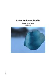
InkPlay: Watercolour Simulation using the Lattice Boltzmann Method ...

Abstract 

InkPlay: 

Watercolour Simulation using the Lattice Boltzmann Method 

for Two-Dimensional Fluid Dynamics 

This paper describes the development of an application 

to simulate various artistic watercolour effects. It uses a 

novel fluid flow model, the Lattice Boltzmann Method 

for the incompressible Navier-Stokes Equation, to 

achieve realistic effects of ink dispersion observed in 

real artwork, including complex flow patterns, light 

fringes and boundary darkening. Unlike most previous 

watercolour simulations the presented solution is not 

concerned with interactive brush stroke input but instead 

creates the effect from a series of TIFF images as a postrender 

process to 2D and 3D animation sequences. The 

various parameters of the simulation and input/output 

options are controlled through a configuration text file. 

CR Categories: I.3.3 [Computer Graphics]: Picture/ 

Image Generation; I.6.3 [Simulation and Modeling]: 

Applications; J.5.0 [Computer Applications]: Arts, fine 

and performing. 

Additional Keywords: Fluid simulation, ink, Lattice 

Boltzmann, non-photorealistic rendering, painting, 

pigments, post-render process, watercolour. 

1 Introduction 

As computer generated images become increasingly 

photo-real, recent years perhaps as a reaction saw a 

heightened awareness of the artistic possibilities of the 

medium. Artists have been using traditional media to 

provide information that may not be readily apparent in 

photographs of real life. To achieve such expressions 

with computer graphics is the motivation of a new field 

of research called non-photorealistic rendering (NPR). 

Watercolour like no other medium captures the spontaneity 

and unpredictable nature of life itself, when the 

motion of water across the paper transports pigments 

along meandering often unexpected paths, forming 

streams and feathery patterns which give it its distinctive 

charm. 

Yet because of this watercolour is perhaps the hardest 

natural medium to simulate as it depends heavily on the 

motion of the pigment solution. It is not surprising therefore 

that the most convincing results have been achieved 

using physically-based models simulating fluid dynamics. 

The traditional approach to fluid simulation uses Navier- 

Stokes Equation solvers which calculate a given number 

Andreas Bauer 

Masters Thesis MSc Computer Animation 2004/2005 

NCCA Bournemouth University 

of individual fluid particles to simulate an overall fluid 

flow. This approach is computationally expensive as the 

quality of the simulation depends on the number of 

particles used with a particular challenge in the Poisson 

equations calculating the pressure redistribution. 

An alternative method for calculating fluid dynamics has 

recently emerged, the Lattice Boltzmann Method, which 

reproduces the Navier-Stokes Equation for incompressible 

flows for small Knudsen and low Mach 

numbers. 

The application developed uses the Lattice Boltzmann 

Method as basis for fluid physics modeling, but extends 

it to simulate the physics of ink flow in absorbent paper. 

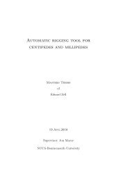
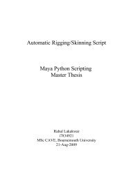
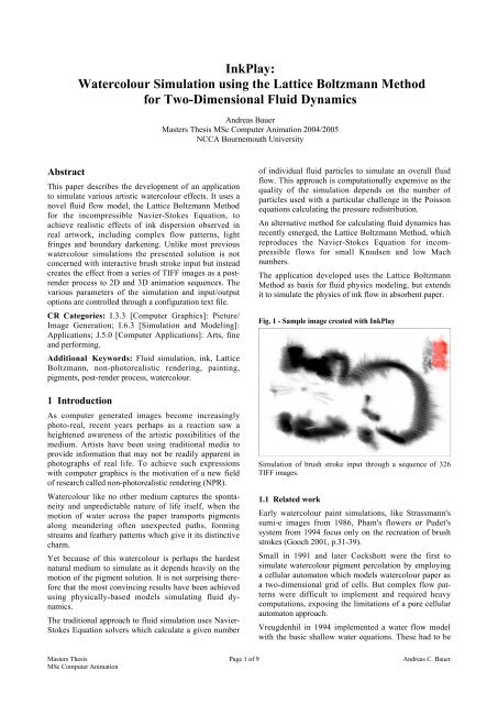
Fig. 1 - Sample image created with InkPlay 

Simulation of brush stroke input through a sequence of 326 

TIFF images. 

1.1 Related work 

Early watercolour paint simulations, like Strassmann's 

sumi-e images from 1986, Pham's flowers or Pudet's 

system from 1994 focus only on the recreation of brush 

strokes (Gooch 2001, p.31-39). 

Small in 1991 and later Cockshott were the first to 

simulate watercolour pigment percolation by employing 

a cellular automaton which models watercolour paper as 

a two-dimensional grid of cells. But complex flow patterns 

were difficult to implement and required heavy 

computations, exposing the limitations of a pure cellular 

automaton approach. 

Vreugdenhil in 1994 implemented a water flow model 

with the basic shallow water equations. These had to be 

Masters Thesis Page 1 of 9 Andreas C. Bauer 

MSc Computer Animation

discretized in time and solved using for example Euler's 

method (Strohotte 2002, p.126). The influence of the 

paper on the flow was realized by adding conditions to 

the equations. 

Curtis expanded Small and Cockshott's approach and 

incorporated some physically-based models but "by no 

means a strict physical simulation" (Curtis et al. 1997). 

But the resulting images were already much more convincing 

than previous approaches. 

At SIGGRAPH 2005 Chu and Tai (2005) presented a 

real-time ink dispersion model rendering on the GPU 

implementing a complete physics-based fluid simulation. 

This paper is based on their work. 

1.2 Overview 

The next section describes the physical properties of 

watercolour and ink painting and gives examples of 

typical effects. Section 3 introduces the Lattice Boltzmann 

Method and section 4 discusses the implementation. 

Finally section 5 discusses observations and some 

ideas for future research. 

2. Physical nature of watercolour and ink 

Using brushes, fingers or other application methods 

artists create expressive lines and shapes, exploiting the 

interaction between water and watercolour to produce 

flowing shades and feathery patterns. 

Any simulation of watercolour on paper needs to deal 

with the two basic items involved: watercolour (or ink) 

and paper. 

2.1 Watercolour and ink 

Writing ink has been used from about 2500 BC, starting 

in Egypt and China. It is typically a mixture of ground 

carbon particles combined with water and a binding 

agent like glue or gum. These agents provide a stable 

liquid suspension of pigment particles and act as a binder 

to fix the pigments during their application on paper to 

prevent them from being removed by mechanical abrasion. 

The higher the glue content the more viscous ink 

becomes. 

Apart from carbon various natural dyes were used, made 

from metals, nuts or seeds, and sea creatures like the 

squid (known as sepia). 

Watercolours use ground colour pigments often from 

precious stones. Watercolour painting began with the 

invention of paper in China shortly after 100 AD. In 

Europe watercolour was introduced in the 16 th century 

and its earlier uses were as thin washes to colourize penand-ink 

or pencil illustrations. 

Pigments can penetrate into the paper, but once in there, 

tend not to migrate far. Lighter pigments travel farther as 

they stay suspended in water longer. Carbon particles are 

much smaller than colour pigments and therefore seep 

into paper fibres easily, giving the most prominent dispersion 

effects. 

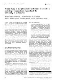
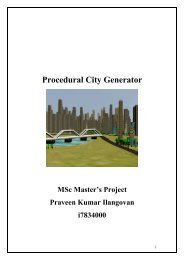
Fig. 2 - Real watercolour effects 

Left: complex flow pattern, right: boundary roughening. 

2.2 Paper 

Paper is mostly air, laced with a microscopic web of 

tangled fibres. It is typically produced from cellulose 

fibres extracted from various woods or plants, processed 

and compacted (Middleton 2003). 

Chinese ink paintings typically use very thin and highly 

absorbent rice paper while watercolour paper is typically 

made from linen or cotton rags. 

It is the structure of the paper that creates the striking ink 

effects. When faced with obstacles, water branches into 

streams and the flowing water carries pigments with it. 

Pigment diffusion plays a minimal role. 

Ink dispersion is also closely determined by paper absorbency; 

it is the imbibition of water that causes the ink 

to flow through the paper fibres. To reduce absorbency, 

the paper can be treated with alum (Chu and Tai 2005). 

3. Lattice Boltzmann Method 

3.1 Historical background 

Over the last few years there has been rapid progress in 

the development of the Lattice Boltzmann Method 

(LBM) for solving a variety of fluid dynamic problems. 

The approach was first proposed 17 years ago by 

McNamara and Zanetti (1988) as an alternative to the 

Lattice Gas Automaton (LGA) for the numerical study of 

the Navier-Stokes equation. 

Although the LBM shares a common origin with the 

LGA it overcomes the latter's shortcomings as it uses a 

set of real-numbered particle velocity distribution functions 

rather than single pseudo-particles with Boolean 

values. As a result the LBM does not exhibit the same 

noise problem as the LGA nor any of the other intrinsic 

flaws of Lattice Gas Automata like violation of Galilean 

invariance or the occurrence of large fluctuations. 

(Galilean invariance is a principle which states that the 

fundamental laws of physics are the same in all inertial 

(uniform-velocity) frames of reference, i.e. all lengths 

and times remain unaffected by the change of velocity. 

(Anon 2005)) 

The initial variant suggested by McNamara and Zanetti 

(1988) was still formulated as a transcript of the lattice 

gas approach with a fixed fluid viscosity. By altering the 

collision terms in the Lattice Boltzmann Equation (LBE) 



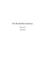
Fig. 3 - Commonly used discretization in 2D and 3D 

Left: D2Q9 lattice, right: D3Q19 lattice 

Bhatnagar, Gross and Krook achieved a single step relaxation 

scheme which replaced the discrete collision 

matrix that had to be formulated in the earlier model. In 

this new Lattice Boltzmann Bhatnagar-Gross-Krook 

method (LBGK) the distribution is relaxed towards a 

local equilibrium distribution function. 

By using a Chapman-Enskog expansion it was shown 

that the LBGK model reproduces the Navier-Stokes 

Equation for incompressible fluids for low Knudsen 

numbers (below 0.1) and low Mach numbers (below 

0.15, i.e. flow speeds below 183.75km/h (114.18mph)) 

(Benzi 1992). 

(The Knudsen number is the ratio between the mean free 

molecule path and a characteristic length scale, for 

example an obstacle size.) 

2.2 The Lattice Boltzmann Method 

The LBM follows a bottom-up approach by simulating 

the evolution of particle distribution functions rather 

than particles themselves. 

The LBM operates on a lattice of square or cubic cells of 

equal size, where each lattice site x at time t stores particle 

distribution functions, ƒi (x, t), along a discrete number 

of velocity vectors ei. In 2D space the most common 

variant uses 9 velocity vectors (8 neighbours and a zero 

vector for the cell itself) and is commonly referred to as 

a D2Q9 lattice. In 3D space the most common lattice 

models are D3Q15 and D3Q19 with 15 or 19 velocity 

vectors depending on whether the longest vectors point 

to the corners of the 3D cube (D3Q15) or to the mid 

point of each cube edge (D3Q19). Figure 3 shows both 

the D2Q9 and D3Q19 lattice. 

Each distribution function ƒi is stored as a floating point 

value and represents the probability of the presence of 

particles in the current cell moving in a velocity vector's 

direction. 

During each time step ∆t two operations are performed at 

each lattice site: 

1.) Streaming ƒis to the next lattice site along their respective 

velocity vectors. 

2.) Colliding ƒis that arrive at the same site. The colliding 

step subsequently computes the effect of the 

collisions which occur during the stream step. The 

collision redistributes towards their equilibrium 

distribution functions ƒi (eq) . 

The two operations of streaming and collision are 

mathematically described by the Lattice Boltzmann 

Equation: 

ƒi (x + ei Δt, t + Δt) = (1 – ω) ƒi (x, t) + ω ƒi (eq) (x, t) Eq. 1 

where ω is the relaxation parameter. 

According to the LBGK model the equilibrium 

distributions ƒi (eq) are: 

3 9 3 

ƒi (eq) = wi ρ + ρ0 c 2 ei · u + 2c 4 (ei · u) 2 – 2c 2 u · u Eq. 2 

where c equals ∆x/∆t, ∆x is the lattice spacing, wi are 

constants determined by the lattice geometry, ρ and u are 

fluid density and velocity respectively, and ρ 0 is a 

predefined average fluid density. 

For a D2Q9 lattice the constants wi are set as 4/9 for the 

zero vector, 1/9 for the velocity vectors pointing north, 

south, east and west, and 1/36 for the diagonal velocity 

vectors of the lattice. 

Fluid density and velocity at each site can be calculated 

from these values by simple summation: 


MSc Computer Animation 

ρ = 

1 

u = ρ0 

8 

∑ ƒi 

i =0 

8 

∑ ei ƒi 

i =1 

Eq. 3 

Eq. 4 

A new set of distribution functions is obtained from a 

weighted average of the streamed distribution functions 

with the equilibrium distribution functions. 

Obstacles are handled by reflecting the particle 

distribution functions at the obstacle boundary, resulting 

in a normal and tangential velocity of zero (bounce back 

scheme). 

2.3 Advantages over Navier-Stokes Solvers 

Giving the same results as the Navier-Stokes Equation 

(within the low Knudsen and Mach limits), Yu (2003) 

pointed out the following advantages of the LBM over 

traditional Navier-Stokes solvers: 

1.) NS solvers need to treat the nonlinear convective 

term, u · ∇u; the LBM totally avoids it as the convection 

becomes simple advection. 

2.) NS equations must solve the Poisson equation for 

pressure which are computationally expensive and 

involve global data communication; the LBM obtains 

pressure through an equation of state and data 

communication is always local lending itself very 

well to parallel computing.

3.) As the Boltzmann equation is kinetic-based, any 

physics associated with the molecular level interaction 

can be easier implemented in the LBM. 

4. Implementation 

4.1 Goal and general considerations 

The key aim for InkPlay was to provide a post-render 

watercolour effect to existing still images or animation 

sequences. It was designed specifically with Ngan-Sum 

Tse's animation masters project in mind as she required 

such an effect. 

This is in contrast to most watercolour implementations 

which usually provide some kind of graphical user interface 

typically a paint brush simulation. 

Not having to implement a graphical user interface has 

the obvious time-saving advantage but there were others 

as well. 

Chu and Tai (2005) had to cut a few corners in their watercolour 

simulation to be able to provide a real-time 

graphical user interface with a guaranteed response time 

of at least 40-44 frames per second. To achieve these impressive 

frame rates, they implemented the fluid 

dynamic simulation on a programmable GPU using a 

series of parallel rendering fragment programs. This 

choice makes sense as the LBM is well suited for 

parallel processing and this also leaves the CPU free to 

handle the brush simulation. But the limiting factor was 

the video memory. With a maximum of 256MB VRAM 

they could only render a simulation resolution of up to 

512 2 pixel. To break this barrier for the user they 

employed texture scaling resizing the image to 3 or 4 

times the simulation resolution and then used real-time 

edge sharpening techniques to re-sharpen the blurred 

outlines. 

To further preserve memory and to be able to use bilinear 

texture interpolation Chu and Tai used 16-bit float 

data types (instead of 32-bit) for all simulation textures. 

This resulted in some precision errors. 

With the decision not to implement a graphical user interface 

for InkPlay, real-time performance was no longer 

a necessity and calculations could be performed in RAM 

allowing for much higher simulation resolutions, only 

limited by RAM. This was important as Ngan-Sum Tse's 

animation required at least the ability to support PAL 

resolution images (720x576 pixel). 

And being not limited by VRAM all simulation textures 

were implemented as 32-bit floats to avoid the precision 

errors Chu and Tai encountered. 

For the 2D fluid dynamic simulation a D2Q9 lattice was 

implemented with e0 the zero vector, e1, e2, e3, e4 the 

nearest neighbour sites (N, E, S, W) and e5, e6, e7, e8 

pointing along the diagonals to the next nearest cells 

(NE, SE, SW, NW). 

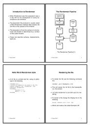
Fig. 4 - Artificial watercolour effects created by InkPlay 

Left: complex flow pattern, right: boundary roughening. 

4.2 Data input / output 

4.2.1 Image input / output 

Without a graphical user interface another means had to 

be found for data input and output. The "Tag Image File 

Format" (TIFF) was chosen for both image input and 

image output for two reasons: 

1.) All major animation and compositing packages support 

TIFFs. 

2.) The flexible TIFF header framework provides additional 

benefits and a route for future expansion. 

One such benefit is the ability to choose from a range of 

compression schemes when opening or saving files. For 

the latter InkPlay offers the user a choice of no compression, 

LZW or JPEG compression. 

TIFF support was implemented with the libtiff library by 

Sam Leffler. 

InkPlay can be supplied with a TIFF image file name as 

parameter when launched from the command line interface. 

The file name must end in either '.tif' or '.tiff' to be 

recognized as a valid TIFF image file. InkPlay will test if 

the image file exists and if so analyze whether the file 

name includes a padded number. 

If a number is found, InkPlay will assume the image file 

to be the first in a sequence of images and attempt to 

load a new image of the sequence in each consecutive 

simulation step. Should an image be missing in the 

sequence InkPlay will simply not add any image to the 

simulation during that simulation step. But it will increment 

the reference index to try loading the next image 

of the sequence in the following simulation step. 

This ability to skip certain images in a sequence provides 

the user with control of when an image is to be applied 

to the simulation. For example when naming three 

images 'image_01.tif', 'image_09.tif' and 'image_21.tif' 

and when supplying InkPlay with the first image's file 

name as parameter InkPlay will apply the first image to 

the simulation during simulation step 1, the second 

image during simulation step 9 and the third image 

during step 21. 

If no padded number was detected in the file name 

InkPlay will apply just this image once to the simulation 

and not look for further images to load. But the simulation 

will be continuously run on that one image. 



If not specified otherwise, InkPlay saves every simulation 

step as an uncompressed TIFF file in a file sequence 

starting with 'image_0000.tif'. 

4.2.2 Control input 

While sufficient in some cases, mere TIFF image input 

does not provide enough control to direct the watercolour 

simulation to achieve specific, desired results. 

InkPlay therefore supports configuration files and includes 

a complete configuration file parser and error 

checker. When launching InkPlay from the command 

line, instead of a TIFF image, a text file can also be 

supplied as parameter: the name of the configuration file. 

If InkPlay is launched without any parameter, a default 

configuration file, 'config.txt', is assumed and InkPlay 

will attempt to load a file of that name from the same 

folder in which InkPlay resides. 

Configuration files allow full access to all simulation 

parameters, a total of 47, to achieve a great variety of 

effects. Support for configuration files also offers an 

easy way to save different sets of settings for later reuse. 

Fig. 5 - Configuration file example 

# This is an example config file 

'Specify the image to load: 

tiff_in, subfolder/image_00.tif 

'Set fluid to average viscosity: 

omega, 0.75 

'Speed up the simulation by 85%: 

speedScale, 1.85 

'Set initial water velocity: 

initialVelocity, 0.05, -0.3 

'Exit simulation after 200 steps: 

simStepExit, 200 

Every configuration file requires at least one parameter, 

tiff_in, which specifies the TIFF image or first image 

of a sequence to be loaded. 

InkPlay's configuration files provides the user with a 

reasonable amount of syntax flexibility. Parameters can 

be in any order and of any number as long as each 

parameter is on a separate line with its values comma- or 

semicolon-separated. Capitalisation of parameters is optional 

so are spaces, tabs and underscores within 

parameter names. Any of these variations is valid: 

tiff_in, TIFF_IN, TIFFin, TiffIn, tiff in, TIFF in 

q_2, Q_2, Q2, q2, q 2, Q 2 

Lines can be left blank and comments can be added by 

starting a line with /, *, #, ', | or !. 

To get a detailed description of all configuration file 

parameters and their syntax the user can launch InkPlay 

specifying '-c' or '--config' as parameter: 

inkplay -c 

Figure 5 shows an example of a short configuration file. 

4.2.3 Information output 

When a simulation is in progress InkPlay provides the 

user with detailed status and progress information in the 

command line window. 

At the start InkPlay displays the approximate amount of 

RAM required and any warnings or errors during startup 

followed by a reminder of allowable keyboard input 

during the simulation. The ten number keys provide 

insight into the status of certain simulation texture and 

data maps by displaying their current status during the 

following simulation step before switching the display 

back to the default output. This allows the user to briefly 

check these parameters. 

4.3 Paper layer simulation 

Chu and Tai (2005) like Curtis et al. (1997) employ a 

three layer simulation model. Contrary to Curtis et al. 

who use a shallow-water, pigment-deposition and 

capillary layer, Chu and Tai's model uses a surface, flow 

and fixture layer. Surface and flow layer each have a 

data map for the water density (amount of water) and 

colour pigments. The fixture layer has only a data map 

for colour pigments. 

4.3.1 Surface layer 

Water, pigments and glue are deposited onto the surface 

layer first. From here they seep into the flow layer. 

As InkPlay does not use a brush simulation, water pigments 

and glue are applied in a stamp- or stencil-like 

fashion one TIFF image at a time. 

TIFF images are expected to be 8-bit RGB byte values 

yet all simulation data maps use 32-bit float data types 

hence TIFF images are first converted from byte to float: 

pixelfloat = pixelbyte / 255 Eq. 5 

And since TIFF images use an additive RGB colour 

model while colour pigments use a subtractive CMY 

colour model, TIFF images are converted from RGB to 

CMY before being applied to the surface layer: 

CMY = {C', M', Y'} = {1 – R, 1 – G, 1 – B} Eq. 6 

InkPlay has full alpha channel support when reading and 

writing TIFF images. If a loaded image does not contain 

an alpha channel, the configuration file parameter 

alphaFromImage can create an alpha channel from the 

image itself where black is considered fully transparent. 

Alternatively the parameter maskingColourRGB can be 

used to specify an RGB value to be considered the transparent 

colour. Any existing or created alpha channel can 

be inverted with the invertAlpha parameter. 

Chu and Tai (2005) did not require support for an alpha 

channel as theirs is a closed system. But when dealing 

with animation sequences support for an alpha channel is 

important. To provide this support, Chu and Tai's model 



has been extended by a fifth channel (next to C, M, Y 

and glue) holding the alpha information. 'Alpha 

pigments' are added in sync with pigments applied to the 

surface layer and advected in sync with pigments moved 

in the flow layer. When saving TIFF images the content 

of this alpha layer is added as the fourth channel. 

To compensate for the lack of a brush that pushes 

pigments into a certain direction, InkPlay allows the 

specification of a 2D velocity vector which is added to 

the simulation when a new TIFF image is applied. 

To model variable paper receptivity, each pixel added is 

masked by the value max(1 – ρ / λ, m) where ρ is the 

water density, λ a receptivity parameter and m a base 

mask value. 

Pigments deposited on the surface layer act as a reservoir 

that provides colour pigment supply to the flow layer. 

4.3.2 Flow layer 

Water gradually seeps in from the surface to the flow 

layer depending on the existing water density in the flow 

layer. 

The amount of water supplied form the surface to the 

flow layer calculates as such: 

ϕ = clamp(s, 0, π – ρ) Eq. 7 

where s denotes the water density in the surface layer, ρ 

the water density in the flow layer and π the capacity of 

the paper fibres. 

Once ϕ is determined, s and ρ are updated accordingly 

and pigments in the flow layer, pf , are updated according 

to the ratio of ρ to ϕ: 

4.3.3 Fixture layer 

pf = (pf ρ + ps ϕ) / (ρ + ϕ) Eq. 8 

Pigments in the flow layer are gradually transferred to 

the fixture layer as the water dries. As real dried ink 

cannot be easily washed away Chu and Tai (2005) 

modelled this transfer to be a one-way process. 

Watercolour pigments on the other hand are easier 

washed away even after the colour dried and it was 

therefore considered to change this transfer into a twoway 

process. But an almost similar effect can be 

achieved by preventing colour pigments from settling 

into the fixture layer in the first place. As this is easily 

done by changing the simulation parameters concerned 

(η, µ and ξ) extending the simulation was considered 

unnecessary. 

4.4 Paper structure simulation 

To accurately simulate paper irregularities Chu and Tai 

(2005) use three helper texture files: the paper grain 

texture, the alum texture and the pinning texture map. 

The LBM does not consider medium permeability or free 

boundary evolution therefore Chu and Tai (2005) made 

several modifications to the basic Lattice Boltzmann 

implementation. 

4.4.1 Permeability 

Variable permeability makes the creation of interesting 

flow patters possible. Permeability is realized by blocking 

the streaming process. Each site is associated with a 

blocking factor κ. Varying κ allows to simulate a wide 

range of media. 

Chu and Tai (2005) use Succi's half-way-bounce-back 

scheme during the streaming process. Blocking is 

performed as if the link to each neighbouring site is partially 

blocked with a blocking factor κ – i which is set to be 

the average of the blocking factors of the two linked 

sites. The streaming step with bounce-back is mathematically 

described as: 

ƒi (x, t + 1) = κ – i (x) ƒk (x, t) + (1 – κ – i (x)) ƒi (x – ei , t) 


MSc Computer Animation 

Eq. 9 

where ƒk is the distribution function pointing in the opposite 

direction of ƒi. 

4.4.2 Viscosity 

In the Lattice Boltzmann Equation viscosity is given by 

(1 / ω – 1 / 2) / 3 assuming that ∆t = c = 1. The lower the 

value for ω the higher the viscosity. 

4.4.3 Paper grain texture 

Voids in the paper fibres and alum deposited determine 

the paper permeability. 

Fibre voids, or paper thickness patterns can simply be 

simulated by scanning a paper grain texture. This 

approach works better than trying to procedurally recreate 

paper structures. A very thin paper, e.g. rice paper, 

was scanned against a black background and the 

resulting image contrast enhanced and finally cropped to 

PAL resolution (720x576 pixel). This texture image, 

'graintexture.tif', is provided with InkPlay. For different 

image resolutions another paper grain texture file needs 

to be prepared. In case InkPlay finds no suitable texture 

file, a new, blank (white) texture image is created and 

used. The texture file provided had been setup for tiling 

so that seamless stitches of any size can be created 

quickly if needed. 

4.4.4 Alum texture 

The alum texture file is used to simulate alum concentration. 

It can easily be created procedurally by 

sprinkling random white dots onto a solid black image. 

InkPlay would not have to use a separate alum texture 

file as it could generate it afresh every time it is 

launched. But this would mean that exact repeatable 

recreations of watercolour effects become impossible. 

Therefore the alum texture, once created, is preserved so 

that InkPlay can use it the next time it is launched.

The blocking factor κ at each site is defined as: 

κ = k1 + k2 G + k3 A + k4 g + k5 h Eq. 10 

where G and A are values from the grain and alum 

texture, ki are weights that define the blocking, g and h 

the glue concentration in the flow and fixture layers. 

4.4.5 Boundary and advection 

Since the effect of air is negligible, a single-phase model 

for water is used. 

The LBM for single-phase models was originally 

designed for the fluid to fill the whole domain. To overcome 

this limitation movable boundaries are introduced, 

where any site can become a boundary site and vice 

versa. A boundary site is a wet lattice site (i.e. ρ > 0) 

with at least one dry site amongst its eight neighbours. 

As the LBM model can cause negative water density for 

empty sites Chu and Tai (2005) reduce the advection 

when the water density gets low. This is done by introducing 

the factor ψ into equation 2: 

3 9 3 

ƒi (eq) = wi ρ + ρ0 ψ 

c 2 ei · u + 4 (ei · u) 

2c 2 – 2 u · u Eq.11 

2c 

ψ = smoothstep(0, α, ρ) Eq. 12 

where α is a parameter for adjusting this effect. 

4.4.6 Pinning texture 

Boundary roughening, or so called 'toes', are caused by 

the spreading front being pinned at different points. A 

front is depinned when there is enough water pressure to 

overcome the pinning. 

Chu and Tai use simple local rules to model pinning and 

depinning which can be efficiently integrated into the 

LBM. 

A site is a pinning site if it is dry and the water density 

ρ at each of the site's eight neighbours is below a 

specific threshold. The four nearest neighbours (north, 

east, south, west) share the same threshold, denoted by 

σ, and the four diagonal neighbours (NE, SE, SW, NW) 

use √ – 2 σ. 

The actual pinning is achieved by setting the blocking 

factor κ to a very high number to fully block all 

neighbouring links. 

To model the effect of paper disorder, a third helper 

texture map is introduced. It is procedurally created by 

sprinkling light, short lines on a black background. 

Modulating s with this texture gives the effect of easier 

ink flow at certain locations and directions. 

Furthermore σ is also made dependent on the glue concentration 

in the flow layer: 

σ = q1 + q2 h + q3 lerp(G, P, smoothstep(0, θ, g)) Eq. 13 

where G and P are values from the grain and pinning 

textures, qi are weights that define the roughening behaviour, 

and θ controls the effect of glue concentration on 

the appearance of toes. The lower θ the lower the glue 

concentration needs to be at which point the result equals 

the pinning texture (i.e. with no contribution from the 

grain map any more). 

Like with the alum texture map InkPlay preserves this 

procedurally created map for later re-use to allow identical 

reproduction of its watercolour effects, if desired. 

4.4.7 Pigment advection 

The movement of pigments is calculated differently 

whether a site is becoming wet in the current simulation 

step or was already wet before. 

For the former pigment concentration newly advected to 

site x is: 

1 

pf *(x) = ρ 

8 

∑ ƒi pf (x – ei ) Eq. 14 

i =1 

For the latter the velocity is back-traced to find out from 

where the pigment arrived: 

pf *(x) = pf (x – u(x)) Eq. 15 

At first look back-tracing might not seem like the best 

approach, but at closer inspection it does make sense: 

Every lattice site has exactly one velocity vector assigned, 

which is the averaged, overall fluid movement 

derived from all ƒis. Tracing these vectors forward 

would break this 1:1 relationship as not every site will 

have one vector pointing to it. Several vectors could 

point to one site leaving other sites as 'holes'. How to fill 

them? And with what pigment colour? And if several 

vectors point to the same site likely some kind of equilibrium 

distribution equation would need to be called 

first, which could result in velocity vectors pointing at 

yet another site, and so on. 

By back-tracing the velocity vectors after the ƒis were 

streamed the 1:1 relationship between a vector and a site 

is guaranteed and every site can be assigned pigments 

from some other site, guaranteeing no holes. 

Back-tracing will likely point to an origin somewhere in 

the middle between four lattice grid points. To find out 

that positions exact pigment concentration a triple linear 

interpolation is done: 

Given the regular 2D lattice grid points A, B, C and D 

(counter clockwise from bottom left) and their respective 

pigment concentrations a, b, c and d, and a point X 

somewhere within those four grid points, the back-traced 

pigment concentration x for point X is: 

temp1 = lerp( d, c, X.x - D.x); 

temp2 = lerp( a, b, X.x - A.x): 

x = lerp( temp1, temp2, X.y - A.y); 



To allow the user to enhance the effect of pigments 

moving, an additional parameter, pfBackDistribution, 

was introduced which is a factor for further redistribution 

of back-traced pigments. 

5 Conclusion 

5.1 Pigment advection speed 

Once InkPlay was implemented it soon became apparent 

that the pigment movement was rather slow and did not 

produce the desired, feathery flow patterns as the equilibrium 

state was reached too quickly. 

Merely increasing the velocity or water density did not 

work as most values are clamped between 0 and 1 for the 

calculations to work and any increase would be clamped. 

To allow for more speed it was decided to decouple the 

velocity u and streaming ƒ is from the rest of the 

calculations. A new parameter was introduced, 

speedScale, which is used to: 

1.) Clamp u and ƒis 

Instead of clamping values between -1 to 1 or 0 to 1, 

values are clamped between -speedScale to 

speedScale or 0 to speedScale. 

2.) 'Translate' between u and ƒis and other parameters 

When deriving other parameters from u or ƒis like ρ, 

u or ƒis are divided by speedScale to bring their 

values back down to the 0 to 1 range. 

This decoupling allows for higher pigment advection 

speeds and dramatically improved the visual appearance 

of the simulation. But it was also found that values 

above 1.85 - 2.0 tend to leave visual gaps between 

simulation steps. Values > 2.0 tend to give even less 

pleasing results. 

In effect the speed gain of the decoupling is only in the 

85-100% range, yet it is still considered a worthwhile 

improvement. 

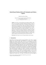
Fig. 6 - Still image from the title sequence of 'Spill + Gush' 

Watercolour effect rendered by InkPlay. 

5.2 'Spill + Gush' 

A main goal for InkPlay was to provide ink spill effects 

for Ngan-Sum Tse's masters animation project. 

She was very pleased with the final result and used many 

InkPlay-created effects in her masters animation project 

5.3 Future Work 

5.3.1 Support for random numbers 

InkPlay currently does not support any random values 

for configuration file parameters. 

This was deliberate to allow for reproducible effects. Yet 

in certain instances a more random approach might be 

desirable. 

5.3.2 Normal render support 

Any velocity currently applied to a TIFF image is 

applied as a one directional vector to the whole image. It 

might be desirable to have a more topologically accurate 

velocity vector, which matches the object depicted. 

With 3D animation normal renders could provide the 

directional information required. But an initial test only 

resulted in unwanted, radial artefacts where normal 

vectors are too close to each other. More testing would 

be needed to find a good application for normal renders. 

Perhaps applying only the rim vectors might work better. 

Figure 7 gives an example of an early normal test render. 

Fig. 7 - Initial test: using a normal render 

Radial artefacts appearing when applying the X and Y vector 

coordinates of a normal image as velocity vectors to the 

simulation. 

5.3.3 Individual advection for each C, M and Y pigment 

Currently all colour pigments are advected at the same 

rate and therefore pigments will never 'split' to blend into 

new colours. Potentially great looking effects could be 

created if CMY pigments would be allowed to advect 

individually. 



As a drawback, the memory footprint would almost 

triple as each pigment will require its own LBM 

simulation. 

Likely the Kubelka-Monk model would have to be used 

to perform the optical compositing of glazing CMY 

layers. 

At that point it might be useful to consider switching the 

colour model to CMYK instead of CMY for added 

effects. 

Acknowledgements 

I would like to thank Prof. John Vince, Dr. Ian 

Stephenson and Dr. Stephen Bell for many helpful 

discussions; James Whitworth for pointing me towards 

useful C++ techniques; and Ngan-Sum Tse for making 

watercolour effects created with my application an 

integral part of her animation masters project. 

References 

ANON, 2005. Wikipedia [online]. Available from: 

http://en.wikipedia.org/wiki/Main_Page 

[accessed on 3 September 2005] 

BENZI, R. et al., 1992. The Lattice Boltzmann Equation: 

Theory and Applications. Physics Reports (Review 

Section of the Physics Letters), 222 (No. 3), 145-197. 

CHU, N. S.-H. and TAI C.-L., 2005. MoXi: Real-Time 

Ink Dispersion in Absorbent Paper. Proceedings of ACM 

SIGGRAPH 2005 [online]. Available from: 

http://doi.acm.org/10.1145/1073204.1073221 


CURTIS, C. J. et al., 1997. Computer-Generated Watercolour. 

Proceedings of the 24th Annual Conference on 

Computer Graphics and Interactive Techniques [online]. 

Available from: 



EBERT, D. S. et al., Texturing & Modeling A 

Procedural Approach. 3 rd ed. San Francisco, California: 

Morgan Kaufmann Publishers. 

GOOCH, B. and GOOCH, A., 2001. Non-Photorealistic 

Rendering. Natick, Massachusetts: A K Peters, Ltd. 

HE, X. and LUO, L.-S., 1997. Lattice Boltzmann Model 

for the Incompressible Navier-Stokes Equation. Journal 

of Statistical Physics, 88, 927-944. 

LANGLANDS, A., 2003. Simulating Watercolour 

Painting. NCCA Bournemouth University Archive, BA 

Computer Visualisation and Animation Research Paper. 

[copy provided by Dr. Stephen Bell.] 

MCNAMARA, G. R. and ZANETTI, G., 1988. Use of 

the Boltzmann Equation to Simulate Lattice-Gas 

Automata. Physical Review Letters, 61 (20), 2332-2335. 

MIDDLETON, M., 2003. Computer Generated Ink with 

Frame to Frame Coherency for Animation. NCCA 

Bournemouth University Archive, BA Computer Visual- 

isation and Animation Research Paper. [copy provided 

by Dr. Stephen Bell.] 

POHL, T. et al., 2004. Performance Evaluation of 

Parallel Large-Scale Lattice Boltzmann Applications on 

Three Supercomputing Architectures. Proceedings of the 

ACM/IEEE SC2004 Conference 2004 [online]. 

Available from: 

http://ieeexplore.ieee.org/iel5/9595/30315/01392951.pdf 

?isnumber=30315&arnumber=1392951 

Digital Object Identifier 10.1109/SC.2004.37 


RAABE, D., 2005. Overview on the Lattice Boltzmann 

Method for Nano- and Microscale Fluid Dynamics in 

Materials Science and Engineering. Max-Planck-Institut 

für Eisenforschung GmbH [online]. Available from: 

http://www.mpie-duesseldorf.mpg.de/forschungProjekte/ 

ProjekteGesamtMU/boltzmann/ 


STILL, M. 2002. Graphics Programming with libtiff. 

IBM developerWorks [online]. Available from: 

http://www-128.ibm.com/developerworks/linux/library/ 

l-libtiff/ 


STOCKMAN, H. W. et al., 2002. Practical Application 

of Lattice-Gas and Lattice Boltzmann Methods to 

Dispersion Problems. Sandia National Laboratories 

[online]. Available from: 

http://www.sandia.gov/eesector/gs/gc/hws/saltfing.htm 


STROHOTTE, T. and SCHLECHTWEG, S., 2002. Non- 

Photorealistic Computer Graphics. San Francisco, 

California: Morgan Kaufmann Publishers. 

SUCCI, S. et al., 1989. Simulations of Three-Dimensional 

Flows with the Lattice Boltzmann Equation on the 

IBM 3090/VF. Proceedings of the 3rd International 

Conference on Supercomputing [online]. Available from: 



TREAVETT, S. M. F. and CHEN, M., 1997. Statistical 

Techniques for the Automated Synthesis of Non- 

Photorealistic Images. Proceedings of the 15th Eurographics 

UK Conference. Norwich, 201-210. 

WEI, X. et al., 2004. Lattice-Based Flow Field 

Modeling. IEEE Transactions on Visualization and 

Computer Graphics, 10 (6), 719-729. 

Also available from: 

http://ieeexplore.ieee.org/iel5/2945/29445/01333669.pdf 

?tp=&arnumber=1333669&isnumber=29445 

Digital Object Identifier 10.1109/TVCG.2004.48 


YU, D. et al., 2003. Viscous flow computations with the 

method of lattice Boltzmann equation. Progress in 

Aerospace Sciences, 39 (2003), 329-367.

InkPlay: Watercolour Simulation using the Lattice Boltzmann Method ...

Create successful ePaper yourself

Delete template?

Save as template?