Observations and Modelling of Fronts and Frontogenesis

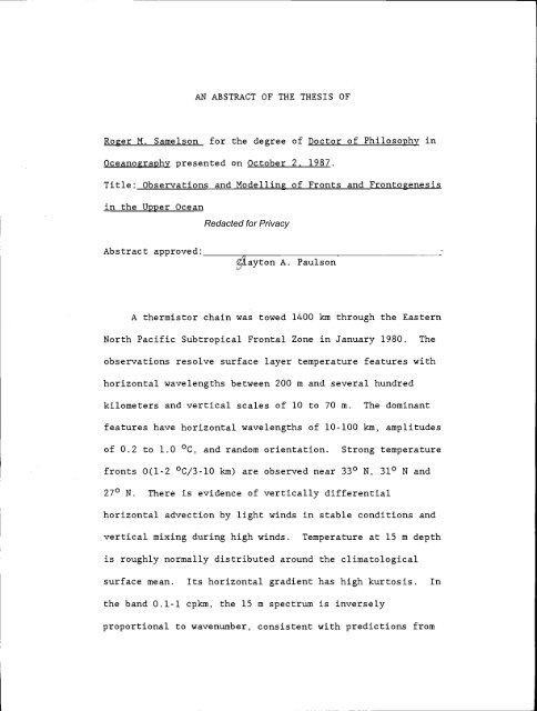
AN ABSTRACT OF THE THESIS OF
Roger M. Samelson for the degree of Doctor of Philosophy in
Oceanography presented on October 2. 1987.
Title: Observations and Modelling of Fronts and Frontogenesis
in the Upper Ocean
Abstract approved:
Redacted for Privacy
ayton A. Paulson
A thermistor chain was towed 1400 km through the Eastern
North Pacific Subtropical Frontal Zone in January 1980. The
observations resolve surface layer temperature features with
horizontal wavelengths between 200 m and several hundred
kilometers and vertical scales of 10 to 70 m. The dominant
features have horizontal wavelengths of 10-100 kin, amplitudes
of 0.2 to 1.0 °C, and random orientation. Strong temperature
fronts 0(1-2 °C/3-lO km) are observed near 330 N, 310 N and
270 N. There is evidence of vertically differential
horizontal advection by light winds in stable conditions and
vertical mixing during high winds. Temperature at 15 m depth
is roughly normally distributed around the climatological
surface mean. Its horizontal gradient has high kurtosis. In
the band 0.1-1 cpkm, the 15 m spectrum is inversely
proportional to wavenumber, consistent with predictions from

the theory of geostrophic turbulence, while the 70 m spectrum
has additional variance consistent with Garrett-Munk internal
wave displacements.
We formulate analytically and solve numerically a
semigeostrophic model for wind-driven thermocline upwelling.
The model has a variable-density entraining mixed layer and
two homogeneous interior layers. All variables are uniform
alongshore. A modified Ekman balance is prescribed far
offshore, and the normal-to-shore velocity field responds on
the scales of the local internal deformation radii, which
adjust dynamically. Sustained upwelling results in a step-
like horizontal profile of mixed layer density, as the layer
interfaces "surface" and are advected offshore. The upwelled
horizontal profile of mixed layer density scales with the
initial internal deformation radii. Around the fronts,
surface layer divergence occurs that is equal in magnitude to
the divergence in the upwelling zone adjacent to the coast,
but its depth penetration is inhibited by the stratification.

Observations and Modelling of Fronts and Frontogenesis
in the Upper Ocean
by
Roger M. Samelson
A THESIS
submitted to
Oregon State University
in partial fulfillment of
the requirements for the
degree of
Doctor of Philosophy
Completed October 2, 1987
Commencement June 1988

APPROVED:
Redacted for Privacy
Professqr of Oceanography in charge of major
Redacted for Privacy
Deane College of Oceanaphy
Redacted for Privacy
Dean of Graduth School
Date thesis is presented October 2. 1987
Typed by researcher for Roger M. Samelson

To my parents, Hans and Nancy Samelson

ACKNOWLEDGEMENTS
I thank my advisor Clayton Paulson and the members of my
committee for their support, guidance, and friendship.
Clayton generously gave me the opportunity to explore a
variety of projects. I owe him a debt of gratitude for his
unwavering personal support. The first half of this thesis
is based on his data; he guided me through its analysis.
Roland de Szoeke suggested the upwelling problem that makes
up the second half of this thesis, and patiently guided me
through it. John Allen invited my cooperation on a separate
project. Doug Caidwell supported me during my first quarter.
Rick Baumann's assistance during the analysis of the
thermistor chain data went far beyond the call of duty. I am
grateful to Jim Richman for conversations concerning the
upwelling problem. Eric Beals and Steve Card provided
comradeship in the trenches while the bits were flying.
Erika Francis, John Leland, Jeff Paduan and others kept me
from going (entirely) off the deep end. Harry Belier taught
me much about the musical routes to chaos. I thank the
scientists and crew of the R/V Wecoma, TH 87 Leg 2, for not
throwing me to the sharks when they had the motive and the
opportunity. Thanks to all those over the years who have
helped me to appreciate that the ocean is more than an analog
device for the solution of certain partial differential
equations of mathematical physics.

This research was supported by ONR under contracts
N00014-87-K-0009 and N00014-84-C-0218 and by NSF under grant
OCE-8541635. Computations for Chapter III were carried out
on the Cray-i at NCAR.

What in water did Bloom, waterlover, drawer of
water, watercarrier returning to the range, admire?
Its universality. . . its vehicular ramifications
in continental lakecontained streams and confluent
oceanflowing rivers with their tributaries and
transoceanic currents: gulfstream, north and south
equatorial courses: its violence in seaquakes,
waterspouts, artesian wells, eruptions, torrents,
eddies, freshets, spates, groundswells, watersheds,
waterpartings, geysers, cataracts, whirlpools,
maelstroms, inundations, deluges, cloudbursts: its
vast circumterrestrial ahorizontal curve: its
secrecy in springs.
James Joyce, Ulysses
Know ye, now, Bulkington? Glimpses do ye seem to
see of that mortally intolerable truth; that all deep
earnest thinking is but the intrepid effort of the soul
to keep the open independence of her sea.. .?
Herman Melville, Moby Dick
Verandahs, where the pages of the sea
are a book left open by an absent master
in the middle of another life.
Derek Walcott, Another Life

TABLE OF CONTENTS
I. INTRODUCTION 1
II. TOWED THERMISTOR CHAIN OBSERVATIONS OF UPPER
OCEAN FRONTS IN THE SUBTROPICAL NORTH PACIFIC 3
Abstract 3
11.1 Introduction 4
11.2 Instrumentation and data collection 6
11.3 Observations 8
11.4 Analysis 14
II.4.a Statistics 14
II.4.b Spectra 16
11.5 Geostrophic turbulence 21
11.6 Summary 26
11.7 References 44
III. SEMIGEOSTROPHIC WIND-DRIVEN THERMOCLINE UPWELLING
AT A COASTAL BOUNDARY 46
Abstract 46
111.1 Introduction 47
111.2 Model formulation 49
III.2.a Equations 49
III.2.b Matching conditions 56
III.2.c Nondimensionalization 60
III.2.d Outline of numerical method 62
111.3 Thermocline upwelling: numerical results
and discussion 65
111.4 Summary 72
111.5 References 82
BIBLIOGRAPHY 83
APPENDIX A: DYNAMICAL DERIVATION OF A MATCHING CONDITION 86
APPENDIX B: NIJMERICAL METHOD 89

LIST OF FIGURES
Fizure Page
11.1 Tow tracks 29
11.2 Hourly sea surface temperature vs. salinity
from on-board CTD during 16-28 Jan., with
contours of 30
11.3 Hourly sea surface temperature, salinity and
from on-board CTD vs. latitude 31
t
11.4 Nominal 15 m (solid) and 70 m (dashed)
thermistor temperature (horizontal 500 m
means) vs. distance along tow tracks 32
11.5 Examples of fronts shown by isotherm crosssections
(interpolated from horizontal 100 m
mean thermistor temperatures) vs. depth and
distance along tow tracks 33
11.6 Probability density of difference of 15 m
temperature from climatological surface
temperature 34
11.7 Probability density of 15 m horizontal
temperature gradient 35
11.8 Horizontal wavenuniber spectrum of horizontal
temperature gradient from Tows 1, 2a, 2b, 3a,
and 4, ensemble averaged and band averaged
to 5 bands per decade 36
11.9 Horizontal wavenuniber spectra of horizontal
temperature gradient from Tows 1, 2a, 2b, 3a,
and 4, band averaged to 10 bands per decade 37
11.10 Horizontal wavenumber spectra of 15 m and 70 m
temperature for Tows 1, 2a, 2b, 3a, and 4,
ensemble averaged and band averaged to 5
bands per decade 38
11.11 Estimated 70 m internal wave vertical
displacement spectra from difference of 70 m
and 15 m power spectra, band averaged to 10
bands per decade (solid lines: x -- Tow 2a,
+ Tow 2b, X -- Tow 4) 39

Figure
LIST OF FIGURES (continued)
Page
11.12 Horizontal wavenuniber spectra and coherence,
ensemble averaged and band averaged to 5 bands
per decade 40
111.1 Model geometry 77
111.2 Nondimensional mixed layer density, layer
depths, and normal-to-shore transport vs.
offshore distance at times t/t* = 8.1 (a-c),
16.0 (d-f), 21.0 (g-i), 25.4 (j-l) 78
111.3 Nondiinensional alongshore geostrophic
velocities at time t/t* 25.4 79
111.4 Nondimensional positions of fronts' vs. time
for Cases 1 (a), 2 (b), and 3 (c) 80
111.5 Nondimensional characteristic curves vs. time
for Case 1 in layers 1 (a), 2 (b), and 3 (c) 81

LIST OF TABLES
Table Page
11.1 Tow start and finish positions and times 41
11.2 Winds and surface fluxes 42
11.3 Climatological sea surface temperature (°C),
averaged over 150-155° W 43

OBSERVATIONS AND MODELLING OF FRONTS AND FRONTOGENESIS
IN THE UPPER OCEAN
I. INTRODUCTION
This thesis comprises two separate projects. The common
theme is fronts and frontogenesis in the upper ocean.
Fronts, regions of unusually large horizontal gradients
in fluid properties, are an important form of physical
oceanographic variability. Though they have received
considerable attention from oceanographers (the recent
monograph The Physical Nature and Structure of Oceanic Fronts
(Fedorov, 1986) contains 279 references), a full
understanding of their role in the ocean still awaits us.
In Chapter II, we present an analysis of upper ocean
temperature data collected near the North Pacific Subtropical
Frontal Zone. In this region of the North Pacific, the
large-scale meridional gradients of temperature, salinity,
and density are intensified in a Frontal Zone. Wind-driven
convergence is the probable primary cause of this
intensification (Roden, 1975). Many small scale fronts are
evident in the data. Baroclinic instability is likely
important in the development of these smaller scale features.
In Chapter III, we present a model for wind-driven
therniocline upwelling at a coastal boundary. In this case,
the action of the wind on the ocean is again frontogenetic.

Here, however, a divergence drives the frontogenesis, as
fluid is drawn up at the boundary to produce horizontal
gradients from vertical stratification.
The basic physics of the upwelling process analyzed in
Chapter III should essentially apply (with appropriate
rescaling and some additional dynamics) to wind-driven
upwelling in the Subarctic gyre north of the Subtropical
Frontal Zone. Since the meridional gradient in surface layer
properties may be partially maintained by this upwelling,
further investigations may eventually link the ideas and
observations of these two Chapters in an unexpected and
relatively direct manner.
2

II. TOWED THERMISTOR CHAIN OBSERVATIONS OF FRONTS
IN THE SUBTROPICAL NORTH PACIFIC
Abstract
A thermistor chain was towed 1400 km through the Eastern
North Pacific Subtropical Frontal Zone in January 1980. The
observations resolve surface layer temperature features with
horizontal wavelengths between 200 m and several hundred
kilometers and vertical scales of 10 to 70 m. The dominant
features have horizontal wavelengths of 10-100 km, amplitudes
of 0.2 to 1.0 °C, and random orientation. Associated with
them is a plateau below 0.1 cpkm in the horizontal
temperature gradient spectrum that is coherent between 15 and
70 m depths. They likely arise from baroclinic instability.
Strong temperature fronts 0(1-2 °C/3-10 km) are observed near
330 N, 31° N and 27° N. Temperature variability is partially
density compensated by salinity, with the fraction of
compensation increasing northward. There is evidence of
vertically differential horizontal advection by light winds
in stable conditions, vertical mixing during high winds, and
shallow convection caused by wind-driven advection of denser
water over less dense water. Temperature at 15 m depth is
roughly normally distributed around the climatological
surface mean, with a standard deviation of approximately 0.7
°C, while its horizontal gradient has high kurtosis and
3

maximum values in excess of 0.25 °C/l00 m. In the band 0.1-1
cpkm, the 15 m spectrum is very nearly inversely proportional
to wavenumber, consistent with predictions from geostrophic
turbulence theory, while the spectrum at 70 m depth has
additional variance that is consistent with Garrett-Munk
internal wave displacements.
11.1 Introduction
The North Pacific Subtropical Frontal Zone is a band of
relatively large mean meridional upper ocean temperature and
salinity gradient centered near 30° N (Roden, 1973). Its
existence is generally attributed to wind-driven surface
convergence and large-scale variations in air-sea heat and
water fluxes (Roden, 1975). A recent attempt has been made
to determine the associated large-scale geostrophic flow
(Niiler and Reynolds, 1984), and hydrographic surveys (Roden,
1981) of the Subtropical Frontal Zone have revealed energetic
mesoscale eddy fields. However, little is known about the
dynamics of the local mesoscale circulation or the detailed
structure, generation, and dissipation of individual frontal
features.
Here we report on an investigation of the upper ocean
thermal structure of fronts in the North Pacific Subtropical
Frontal Zone. We use the term "Frontal Zone" rather than
"Front" because these wintertime measurements show randomly
4

oriented multiple surface fronts up to 2 °C in magnitude and
less than 10 km in width. Observations were made in January
1980 with a towed thermistor chain that measured temperature
at 12 to 21 depths in the upper 100 m of the water column.
The thermistor chain was towed a distance of 1400 km in an
area of the Pacific bounded by 26° and 340 N, 1500 and 158°
W. The observations resolve surface layer temperature
features with horizontal wavelengths between 200 m and
several hundred km and vertical scales of 10 to 70 m. The
towed thermistor chain and data collection procedure are
described in Section 11.2. Section 11.3 is devoted to a
description of the fronts, their magnitude and horizontal
scales, temperature-salinity compensation, vertical
stratification, and response to wind. Probability densities
of surface (15 m) temperature (with the climatological mean
removed) and surface temperature gradient are presented in
Section II.4.a. Horizontal wavenumber spectra of temperature
and temperature gradient at several depths between 15 and 70
m are presented in Section II.4.b. In Section 11.5, the high
wavenumber tail of the temperature spectrum is compared with
the predictions of the theory of geostrophic turbulence
(Charney, 1971). Section 11.6 contains a summary.
5

11.2 Instrumentation and data collection
The thermistor chain tows were made during FRONTS 80, a
multi-investigator endeavor focused on the Subtropical
Frontal Zone near 310 N, 155° W, in January 1980. Other
measurements by other investigators included CTD surveys
(Roden, 1981), remotely sensed infrared radiation (Van
Woert, 1982), XCP velocity profiles (Kunze and Sanford,
1984), and drifting buoy tracks (Niiler and Reynolds, 1984).
The thermistor chain has been described in Paulson et
(1980). The chain was 120 m long, with a 450 kg lead
depressor to maintain a near vertical alignment while it was
towed behind the ship. Sensors were located at approximately
4 m intervals over the lower 82 m. These sensors included 27
Thermometrics P-85 thermistors and three pressure
transducers. The thermistors have a response time of 0.1 s,
relative accuracy of better than iO3 °C, and absolute
accuracy of roughly 10-2 °C. Data were recorded at a
sampling frequency of 10 Hz. For this analysis, individual
thermistor data records were averaged to values at 100 m
intervals using ship speed from two-hourly positions
interpolated from satellite fixes. Since this speed varied
(from 2 to 6 m s1-), the averaged values contain a variable
number of data points (from 166 to 502). The averaging
removes the effects of ship roll and pitch and surface

gravity waves. A maximum of 21 and a minimum of 12
thermistors functioned for entire tows. Thermistor depths
were obtained from the ship's log speed and a model of the
towed chain configuration calibrated by data from the
pressure transducers. Temperature measurements were obtained
at maximum and minimum depths of 95 m and 4 m.
The tow tracks are displayed in Figure 11.1. The four
tows are labeled by number in chronological order. Since the
tracks for Tows 2 and 3 overlap, the track for Tow 3, which
took place on 25 January, is displayed separately, overlaid
on a contour of temperature at 20 m from the Roden CTD survey
during 24-30 January. Tows 2 and 3 are each divided into
sections, labeled a and b, by course changes. The tow start
and finish positions and times are given in Table 11.1.
During 19-26 January, the ship remained within the rectangle
indicated by dashed lines in Figure 11.1.
Surface salinity was determined from temperature and
conductivity measured by a Bisset Berman CTD located in the
ship's wet lab, to which water was pumped from a sea chest at
approximately 5 m depth. The cycle time for the fluid in
this system was roughly 5-10 minutes during most of the
experiment. The CTD temperature, corrected for
(approximately 1 °C) intake warming by comparison with data
from the uppermost thermistor, was used to obtain surface
density. CTD conductivity and temperature were recorded
7

hourly (once every 10-20 km at typical tow speeds), as were
surface wind speed and direction (from an anemometer at 34.4
m height), dry and wet bulb air temperatures, and incident
solar radiation.
11.3 Observations
Sea surface temperature and salinity from ship-board CTD
measurements during 16-28 January are displayed with contours
of at (density) in Figure 11.2. The data range over 7 °C in
temperature (T) and 1 ppt in salinity (S). Though
temperature may vary by 1 °C at constant salinity, most of
the data approximately obey a single identifiable T-S
relation, with the exception of four points with T > 20.5 °C,
S . 35.1
ppt, which occurred after the encounter of a strong
front at the southern end of Tow 4. Salinity tends to
compensate temperature, so the density variations are small,
but relative temperature still tends to indicate relative
density (warmer, more saline, water is typically less dense).
Surface temperature, salinity, and at are displayed
versus latitude in Figure 11.3. Scales have been chosen
using the equation of state so that a unit distance change in
temperature (salinity) at constant salinity (temperature)
corresponds approximately to a unit distance change in at.
Temperature and salinity tend to decrease toward higher
latitudes. The corresponding density gradient is relatively

small, since the large-scale temperature and salinity
gradients are density-compensating. Features with smaller
horizontal scales also show compensation. A front near 300 N
was crossed several times during 19-27 January and appears as
a noisy step-like, partially compensated, feature. (Its
apparent sharpness is exaggerated by a set of measurements
taken during frontal transects at constant latitude.) The
large temperature feature near 330 N is roughly 70%
compensated by salinity. In contrast, the 2 °C front near
27° N has negligible salinity variation. There appears to be
a density feature with roughly 300 km wavelength between 310
N and 34° N.
For each of the tows, Figure 11.4 displays traces of 500
m horizontal averages of nominal 15 m (solid line) and 70 m
(dashed line) thermistor temperature. These are respectively
the shallowest and deepest depths at which thermistor
measurements were made during all four tows. The dominant
temperature features have horizontal wavelengths of 10 to 100
km, amplitudes of 0.2 to 1.0 °C, and no apparent preferred
orientation with respect to the large-scale (climatological)
temperature gradient. Satellite imagery of the Subtropical
Frontal Zone in January and February 1980 (Van Woert, 1981,
1982), some of which is precisely simultaneous with the tows,
shows a sea surface temperature field composed of highly
distorted isotherms, such as result from advection of a

tracer by a strain field, rather than a collection of
isolated patches of random temperature. The thermistor chain
tows are cross-sections of this field. On horizontal scales
of hundreds of kilometers, several large fronts, across which
the temperature change (roughly 1 °C or more) has the same
sign as the large-scale gradient, give a step-like appearance
to the temperature record.
The salinity-compensated temperature structure that
dominates Tow 1 is visible near 33° N in Figure 11.3.
Measured horizontal temperature gradients exceeded 0.25
°C/lOOm in the front near 110 km, the largest observed during
the experiment.
In Tow 2a, a large front was encountered at 200 km, near
300 N. The feature in Tow 2b near 70 km appears to be a
meander of the same front. This meander is visible in
infrared satellite imagery from 17 January 1980 (Figure 2a,
Van Woert, 1982).
Tow 3, made on 25 January, was contained in the region
covered by a CTD survey (Roden, 1981) during 24-31 January.
The tow is roughly perpendicular to the isotherms of the
surveyed front (Figure II.lb). The mean temperature gradient
is large over this entire tow. The sharp frontal boundary
near 18 °C observed a week earlier at the same location
during Tow 2a, does not appear in Tow 3. A tongue of warm
water was crossed at the southern end of the tow, with a
10

front at about 18.5 °C. There is frontal structure near 60
kin, at about 17.5 0C, in both Tows 3a and 3b. Note the
similarity of Tows 3a and 3b, which were made on the same
track (in opposing directions) but several hours apart.
The largest temperature front encountered during the
experiment, with horizontal gradient reaching 1.5 °C/3 km and
a temperature change of roughly 2 °C over 10 kin, occurred
near 27° N at 350 km in Tow 4. The salinity change across
this feature is small and in fact enhances the density
change, which is approximately 0.5 kg m3 over 10 km, most of
it occurring over 3 km. This is larger than the density
variability observed over the entire remainder of the
experiment. Isotherm cross-sections of this front are shown
in Figure II.5a. The geostrophic vertical shear across the
front is roughly 10-2 s- at the surface. Large amplitude
internal wave vertical displacements of the seasonal
thermocline are visible.
The vertical temperature gradient between 15 m and 70 m
was generally weak except in regions near frontal features.
During Tow 1, appreciable vertical gradients appear only
within 10-15 km of the fronts. During Tow 2, some vertical
gradients occur up to 25-30 km from fronts (though there may
be closer fronts that lie off the tow track). The upper 70 m
are nearly homogeneous in temperature over most of Tow 3a. A
small amount of stratification is evident near features
11

etween 50 and 75 km and in the warm tongue near 110 km.
These features and the associated vertical gradients are
evident as well in Tow 3b, which followed the same track on
the opposite course. In Tow 4, as in Tows 1 and 2, vertical
gradients are found consistently near frontal features.
Often the upper sections of individual fronts appear
displaced horizontally by several kilometers from the lower
sections. During Tow 2, particularly over the interval
125-300 km, 15 m temperatures have traces that are similar to
the 70 in temperatures but offset to the north. Winds (Table
11.2) during 17 January were from the south, and may have
displaced a shallow layer northward and eastward. Isotherm
cross-sections of the feature near 135 kin are shown in Figure
II.5b. (Note that the presence of a temperature inversion
implies an anomalous local T-S relation, according to which
the warmer, more saline water is denser.) The displacement
can only be estimated, since the angle of incidence of the
tow track across the front is unknown, but it appears to be a
few kilometers. This is an appropriate value for Ekman layer
flow in response to light winds whose direction varies on a
2-5 day time scale, and is typical of such features in the
data, most of which occurred after periods of light winds.
Estimates of daily average buoyancy flux, made from hourly
bulk estimates of surface fluxes, are shown in Table 2, and
Monin-Obukhov depths calculated from the flux estimates are
12

given in the stable cases (downward buoyancy flux). The
uncertainty in the flux estimates is roughly 20%. The
Monin-Obukhov depth for 17 January, the date of the
observations shown in Figure II.5b, is 62 m. This is
comparable to the depth of the displaced upper section.
Convection in the mixed layer may have prevented a similar
structure from forming as wind stress forced denser fluid
over less dense fluid at the right-hand front in Figure 5b.
Vertical gradients in the surface layer are negligible
over the last 70 kin of Tow 2 in spite of horizontal gradients
as large as those over the first 540 km. During this last
period of Tow 2b, local wind speeds rose from 5-10 m s to
20 m sfl-, where they remained until after the tow was
terminated. (Table 11.2 gives daily vector averaged hourly
winds; daily average magnitudes are larger.) The surface
layer is nearly uniform in temperature to 70 m depth over
most of Tow 3 as well. Maximum wind speeds of 20 m s were
attained in this region two days prior to Tow 3. The absence
of vertical gradients during these two periods is likely due
to vertical mixing in response to the high winds. Tow 3 was
taken along part of the line covered by Tow 2a and runs
between the locations of hydrographic stations occupied by
the CTD survey (Roden, 1981). The surface temperature in
this region decreased by approximately 1 °C between Tows 2a
and 3. Roden (1981) interprets this decrease as southward
13

advection of a tongue of cold water in a frontal meander, but
cooling by entrainment may also have contributed. Large
(1986) present evidence for large entrainment events in
the North Pacific during the fall season. These appear to be
shear mixing events driven by the near-inertial response to
storms.
A 0.7 °C temperature inversion, roughly 5 kin wide,
occurred at 100 kin, near the well-compensated front
encountered during Tow 1. Isotherm cross-sections of this
feature are displayed in Figure II,5c. The presence of an
inversion implies an anomalous local T-S relation, according
to which the warmer, more saline water is denser. The warm,
dense water most likely originated from the warm side of the
front, with which it may be contiguous. The wind record
(Table 11.2) suggests an Ekman flow to the southeast, nearly
normal to the tow track, so that the cooler surface water may
have been advected over the warmer water from the northwest.
II.4.a Statistics
11.4 Analysis
To characterize the temperature variability
statistically, we have calculated probability densities of
temperature gradient and temperature deviation from
climatology. Table 11.3 lists climatological surface
14

temperatures for January and February from 100 years of ship
observations and 27 years of hydrocasts (Robinson, 1976).
Figure 11.6 shows the probability density of the deviation of
15 m temperatures from a fit, linear in latitude in the
intervals 253O0 N and 30-35° N, to the January climatology.
As noted by Roden (1981), the surface layer temperatures are
colder on average than the climatological means. The
apparent bimodality is probably due to poor statistics. The
standard deviation is roughly 0.5 °C. Relative to the
climatological gradient, this would correspond to an
adiabatic meridional displacement of 80-100 km. From
drifters deployed near 30° N, 150° W, Niiler and Reynolds
(1984) compute a mean northward surface velocity of 1-2 cm
s1- during 27 January through 30 April 1980. From infrared
imagery, Van Woert (1982) estimates an e-folding time of 60
days for a large frontal meander near 30 N during January and
February 1980. The meridional displacement scale is
comparable to the product of these velocity and time scales.
Standard mixing-length arguments yield an eddy diffusivity
(as velocity times length or length squared divided by time)
of 1-2 x l0 m2 s1-. This is an order of magnitude smaller
than typical values used in numerical models (e.g., Lativ,
1987)
Horizontal 100 m mean temperature gradients were
calculated from differences of adjacent 15 m temperatures.
15

Figure 11.7 displays the probability density of these
gradients. The dotted line represents a Gaussian
distribution with the observed mean and standard deviation.
The observed kurtosis is 76, much larger than the Gaussian
value of 3. This suggests the presence of a velocity field
that strains the temperature gradients to small scales. The
large kurtosis is characteristic of processes with sharp
transitions between small and large values. It measures the
front-like nature of the surface temperature field, which is
dominated by intermittent large gradients separated by
regions of small gradients. Qualitatively similar
distributions of temperature and velocity gradients occur at
small scales in three-dimensional turbulence (Monin and
Yaglom, 1975). Calculations of the kurtosis for
distributions of average horizontal gradient over distances
from 100 m to 100 km show that the kurtosis increases sharply
below scales of 10 km, with an evident but irregular change
in dependence at a few hundred meters, roughly the vertical
scales of the surface boundary layer.
II.4.b Spectra
Figure 11.8 displays the ensemble averaged horizontal
wavenumber spectrum of 15 m horizontal temperature gradient,
band averaged to 5 bands per decade. The variability between
10 and 100 km wavelengths that is evident in the time series
16

dominates the spectrum. At these wavenumbers and at
wavenumbers above 1 cpkm, the spectrum is approximately
constant. Between 0.1 cpkm and 1 cpkm, the spectrum is very
nearly proportional to k1-, where k is wavenumber.
We associate the low wavenumber plateau with the
mesoscale eddy field, the likely source of the dominant
temperature features. The constant spectral level is a
typical signature of an eddy production range, which may be
driven by baroclinic instability. This instability generally
prefers the scale of the internal deformation radius. The
first local internal deformation radius, calculated using a
FRONTS 80 CTD station for the upper 1500 m supplemented by
deep data from a 1984 meridional transect, is 40 km, which
lies within the energetic plateau, toward its less resolved
low wavenumber end. The break in slope at the high
wavenumber end of the plateau occurs near 0.1 cpkm, at
roughly the fifth internal deformation radius. The constant
spectral level at wavenumbers above 1 cpkm is likely due to
temperature gradient production in the surface boundary
layer.
Figure 11.9 displays horizontal wavenumber spectra of 15
m horizontal temperature gradient from each individual tow,
band averaged to 10 bands per decade. The spectral levels
vary by roughly half a decade. The spectral shapes are
nearly uniform, despite the apparent difference in the
17

qualitative nature of the records noted in Section 11.3
(e.g., the single large feature in Tow 1 versus the myriad
smaller features in Tows 2a, 2b). Each spectrum has a broad
peak or plateau at low wavenumber, a break in slope near 10
km, and is approximately proportional to k1- between 10 km
and 1 km. A minimum occurs between 1 km and 350 m
wavelengths in three of the five spectra. A secondary peak
appears near 350 m in these three spectra, followed by a
decrease toward the Nyquist wavelength (200 m). The spectra
appear to fall off slightly toward wavelengths larger than 50
km. In this region however the number of data points is
small and the 95% confidence intervals large. The spectrum
from Tow 3b is not shown. At the 95% confidence level, it is
essentially indistinguishable from the Tow 3a spectrum.
Because of the close time and space scales, we interpret this
as a lack of independence between the two spectral estimates
from Tow 3, and have only included the estimate from Tow 3a
in the ensemble average.
Figure 11.10 displays ensemble averaged horizontal
wavenumber spectra of 15 m and 70 m temperature, band
averaged to 5 bands per decade. We interpret the difference
between the spectral levels at 15 m and 70 m in the bands
above 0.1 cpkm as internal wave vertical displacements at 70
m. Since the average vertical temperature gradients are
small at 15 m (less than l0 0C ma-; at 70 m they are
18

typically iO-2iO3 °c m1-), and since the vertical internal
wave velocities must vanish at the surface, temperature
variance from internal wave isotherm displacements will be
small at 15 m. If the 70 m spectrum is composed of the sum
of an internal wave vertical displacement spectrum that is
uncorrelated with the 15 m spectrum and a spectrum (due to
other processes) equal in variance to the 15 m spectrum at
each wavenumber, the 70 m internal wave spectrum will be the
difference of the power spectra at 70 m and 15 m.
(Differencing the series leads to an overestimate of the
internal wave variance, as incoherent parts not due to
internal waves will contribute to the power spectrum of the
differenced series.) Using average vertical temperature
gradients at 70 m from entire tow means of surrounding
thermistors to estimate displacements and the local buoyancy
frequency, we obtain for Tows 2 and 4 the internal wave
energy spectral estimates shown in Figure 11.11. The
empirical Garrett-Munk prediction (Eq. Al2, Katz and Briscoe,
1979; Garrett and Munk, 1972), with Desaubies (1976)
parameters r 320 m2 h1- and t = 4 x l0 cph cpm-, is
plotted for comparison. The spectral levels are mostly
within 2 to 3 times the predicted values, and the spectral
slopes show excellent agreement. A large temperature
inversion and small vertical gradients prevented reliable
calculations for Tows 1 and 3. Even in Tows 2 and 4, average
19

temperature differences of surrounding thermistors are not
far from the noise level of the calibrations, so these
estimates have limited value as measurements of internal wave
energy. They are however consistent with the assumption that
the difference in the 70 m and 15 m spectral levels in the
0.1-1 cpkm band is due to internal waves, and that the
variance in the 15 m spectrum in this band is due to other
processes. Below 0.1 cpkm, where the break in slope in the
15 m spectrum occurs, the internal wave energy appears to
fall off. This apparently fortuitous correspondence gives
the 70 m spectrum a nearly uniform slope (Figure 11.10).
Figure 11.12 displays ensemble averaged spectra of
horizontal temperature gradients at 15, 23, 31, 50, and 70 m,
as well as ensemble averaged coherence from cross-spectra
between the 15 m record and the others, all band averaged to
5 bands per decade. There is significant vertical coherence
in the 0.1-1 cpkm band over most of the surface layer. Where
the internal wave variance raises the spectral levels above
the 15 m values, coherence is rapidly destroyed. This occurs
at successively shorter wavelengths as the vertical
separation decreases, presumably since only short wavelength
internal waves may exist on infrequent shallow patches of
vertical gradient.
20

11.5 Geostrophic turbulence
We have interpreted the low wavenumber plateau in the 15
m horizontal temperature gradient spectrum (Figure 11.8) as
the signature of the mesoscale eddy field and a probable
baroclinic production range, and the high wavenumber plateau
as a surface boundary layer production range. At wavenumbers
above 0.1 cpkm, internal waves consistently account for the
difference between the 70 m and .15 m spectra (Figures 11.10
and 11.11). It remains to identify the source of the
additional temperature variance in the 0.1-1 cpkm wavenuniber
band. In this band, the temperature gradient spectrum has
95%-significant vertical coherence and is very nearly
proportional to k1- (Figures 11.8 and 11.9). Charney (1971)
predicted a k3 subrange in the potential energy spectrum
above a baroclinic production range. If the potential energy
spectrum has the same slope as the temperature spectrum in
the 0.1-1 cpkm band, the observations will be consistent with
this prediction, since the temperature spectrum (Figure
11.10) is proportional to times the temperature gradient
spectrum.
Charney (1971) discovered a formal analogy that holds
under certain conditions between the spectral energy
evolution equations associated with the two-dimensional
Navier-Stokes equations and the quasigeostrophic potential
21

vorticity ('pseudo-potential vorticity') equation, and
inferred the existence and spectral form of an inertial
subrange in quasigeostrophic motion from the results of
Kraichnan (1967) on two dimensional Navier-Stokes turbulence.
In this subrange, enstrophy (half-squared vorticity) is
cascaded to small scales, rather than energy as in
three-dimensional turbulence. Charney (1971) introduced the
phrase 'geostrophic turbulence' to describe the energetic,
low frequency, high wavenumber, three-dimensional,
near-geostrophic motions to which this theory applies. The
phrase is now also used more generally to describe the
'chaotic, nonlinear motion of fluids that are near to a state
of geostrophic and hydrostatic balance' (Rhines, 1979) but in
which anisotropic waves (e.g., Rossby waves) may also
propagate.
In the predicted inertial subrange, the energy spectrum
E(k) has the form
E(k) = c ,2/3 k3,
where C is a universal constant, r is the enstrophy cascade
rate, and k is an isotropic wavenumber. Total energy is
equally distributed between the potential energy and each of
the two components of kinetic energy. For a spatially
oriented wavenumber (e.g., wavenuniber along a tow track), the
power law dependence is unchanged, but the transverse
velocity kinetic energy component contains three times the
22

energy of each of the longitudinal component and the
potential energy component, so the total energy is five times
the potential energy (Charney, 1971).
The potential energy may be expressed in terms of the
density, using the hydrostatic balance and a local value of
the buoyancy frequency N:
(Potential energy) (g/N)2((p
where g is gravitational acceleration, p is density, and p
is a constant reference density. Temperature and salinity
data (Figure 11.2) indicate that relative temperature tends
to determine relative density, at least on the 10-15 km
scales of the salinity data. We have used linear regression
T-S relations from these data to convert 15 m temperature to
density. For Tow 1, a single linear T-S relation was used,
for Tow 2, three relations, for Tow 3, a single relation, and
for Tow 4, three relations. The change in spectral shape
from this conversion was minimal. The spectral levels were
altered, with Tows 2 and 3 nearly equal and Tow 1 roughly
half, Tow 4 roughly three times as large as Tows 2 and 3.
(The large front near 260 N is intensified by the conversion
to density and was excluded from the density spectra, as it
imparts a strong k2 signal to the spectrum and appears to
beldng to a dynamical regime different from that of the
remainder of the observations.)
23

A relatively large uncertainty is associated with the
choice of a value of N for the conversion from density to
potential energy. The Charney theory requires use of the
local N, which is assumed to be slowly varying. In the mixed
layer, N may be arbitrarily small, and at the mixed layer
base, N is not slowly varying. We use a moderate value of 2
cph. Within the 95% confidence intervals, the resulting
ensemble averaged potential energy spectrum may be obtained
directly by multiplying the 15 m temperature spectrum in
Figure 11.10 by lO cm s2 oC2. The variance in the 0.1-1
cpkm band is roughly 3 cm2 s2, the corresponding predicted
kinetic energy 12 cm2 s2. A velocity scale U formed from
the square root of twice the kinetic energy is 5 cm sfl-,
which yields a Rossby number (Uk/f = 0.05 at k 0.1 cpkm)
that is appropriate for quasigeostrophic theory. Assuming
the universal constant C is equal to one, we estimate the
potential enstrophy transfer (dissipation) rate as 2xl0-6
s3. This lies between atmospheric estimates of 10-15 s3
(Charney, 1971; Leith, 1971) and numerical ocean model values
of 5xl0-9 s3 (McWilliams and Chow, 1981).
The interpretation of the 0.1-1 cpkm band as a
geostrophically turbulent inertial subrange appears to be
consistent with the theory. There is considerable
uncertainty in the conversion of temperature to density and
potential energy. The predictive theory requires a slowly
24

varying N and a flow isolated from boundary effects; these
conditions may not apply here, but it is not evident that
they are essential to the dynamics.
The rins temperature
amplitude (square root of the variance) in the band is
roughly 0.05 °C. This is 50 times the thermistor noise
level, but it is a small physical signal that could be
created by relative meridional displacements of five to ten
kilometers in the mean field. Some possible alternative
mechanisms are:
(1) Internal waves. At 15 m depth, horizontal
displacements by high frequency internal waves should be
small. Lagrangian motion due to near-inertial waves and
wind-driven surface currents, which will depend strongly on
the horizontal structure of the velocity fields, is not well
understood and may contribute to the observed variance.
(2) Variations in air-sea fluxes and entrainment. At
horizontal scales below 10 km, variations in air-sea fluxes
should not be sufficient to create 0.05 °C features in a
mixed layer of 75-125 m depth. (This would require a
differential heat flux of 200 W m2 over a day.) Note that
variations in mixed layer depth may produce temperature
variations in response to even a spatially constant heat
flux. Variations in entrainment, such as those observed by
Large (1986), similarly may produce mixed layer
25

temperature variations, but again presumably mostly on scales
larger than 10 km.
Over 900-km space and two-week time scales and despite
variable atmospheric conditions, the spectral shapes were
roughly constant. This suggests that processes that
contribute substantially to the variance must be
statistically homogeneous over these scales. Near-inertial
currents, which respond strongly to storms, would appear not
to meet this criterion.
Finally, we note that the -3 power law temperature
spectrum differs from that predicted for a passively advected
scalar in a turbulent flow. In that case the scalar
spectrum, not the gradient spectrum, is inversely
proportional to wavenumber (atchelor, 1959).
11.6 Summary
The thermistor tows yield a detailed two-dimensional
description of surface layer temperature along 1400 km of tow
tracks in the Eastern North Pacific Subtropical Frontal Zone
during January 1980. In brief, we find:
(1) The dominant features have wavelengths of 10-100 km,
amplitudes of 0.2 to 1.0 °C, and no preferred orientation
with respect to the mean meridional gradient (Figure 11.4).
These features, which could be created from the
climatological mean sea surface temperature field by
26

adiabatic meridional displacements of roughly 100 km, likely
arise from baroclinic instability of the geostrophic upper
ocean flow. They form a plateau in the temperature gradient
spectrum at wavelengths above 10 km (Figure 11.8).
(2) Strong temperature fronts are observed near 330 N, 310
N and 27° N, with density compensation by salinity increasing
northward (Figures 11.3,4). Maximum horizontal near-surface
gradients exceed 0.25 °C/l00 m (Figure 11.7). There is
evidence of vertically differential horizontal advection in
the surface layer by light winds (Figure II.5b), enhanced
vertical mixing during periods of strong winds, and shallow
(100-200 m depth) convection caused by wind-driven advection
of a dense layer over a deep less-dense layer.
(3) Temperature is roughly normally distributed around the
climatological mean (Figure 11.6). The near-surface
horizontal temperature gradient has high kurtosis (Figure
II . 7)
(4) The high horizontal wavenumber (0.1-1 cpkm) tail of the
near-surface temperature spectrum has the -3 power law form
(Figures 11.8,10) predicted by Charney (1971) for energetic
high wavenumber near-geostrophic motion above a baroclinic
production range. Horizontal temperature gradients have
significant vertical coherence over the upper 50 m at all
wavelengths and over the upper 70 m at wavelengths greater
than 5 km (Figure 11.12).
27

(5)
The departure at 70 m depth of the temperature spectrum
from the -3 power law can be ascribed to internal wave
vertical displacements that are consistent with the Garrett-
Munk model of the internal wave spectrum (Figure 11.11).
28

z0
34
32
V
v 30
a
-J
28
26
a)
- 2b$'
4
2a
I I I
156 154 152 150
Longitude (°w)
-
z0
V
0
111
4-,
0
-J 30
41
b)
/ 30
I I
154 153
Longitude (°W)
Figure 11.1 Tow tracks. + -- two-hourly positions. (Table
1 lists start and finish positions and times.)
a) Tows 1, 2a, 2b, and 4. Ship remained
within dashed rectangle during 19-26 Jan.
b) Tows 3a and 3b. Isotherms at 20 m from CTD
survey (Roden, 1981).
N-)

00
22
20
16
14
34.0 34.5 35.0 35.5
Solinity (ppt)
Figure 11.2 Hourly sea surface temperature vs. salinity
from on-board CTD during 16-28 Jan., with
contours of
30

U0
V
L
0
L
V
20
E 16
V
12
p
;
t *,
S
:,,, ,,
T
* N
.isø U
I ..IpS p
1
26 28 30 iZ
Latitude (°N)
Figure 11.3 Hourly sea surface temperature, salinity and at
from on-board CTD vs. latitude.
at
K
L)
I-

20
19
18
18
17
16
15
0 50 100 150
Tow 1 (16 Jon 80)
0 50 100 150 200 250 300 350 400
Tow 2c (17-18 Jan 80)
18
0 50 100 150 200 0 50 100 0 50
km km km
22
21
20
Figure 11.4
low 2b (18-10 Jon 80) Tom 3o (25 Jon 80) low 3b (25 Jon 80)
0 50 100 150 200 250 300 350 400
Tom 4 (27-28 Jon 80)
Nominal 15 m (solid) and 70 m (dashed)
thermistor temperature (horizontal 500 m means)
vs. distance along tow tracks. The large
fronts in Tow 1 near 125 kin, Tow 2a near 200
km, and Tow 4 near 350 km are visible in Figure
3 near 33° N, 310 N, and 27° N, respectively.
32

30
E 50
-c
a-
I,
0
70
90
300 360 370 380
Distance (i

0
I..
0
1.20
0.80
0.40
3.0 2.0 1.0 0.0 1.0
Figure 11.6
T (°c)
Probability density of difference of 15 m
temperature from climatological surface
temperature. Area under curve Is fraction of
occurrence. Dashed line: Gaussian
distribution with same mean and standard
deviation.
34

10
10°
10-2
1 0
-3.0 -2.0 -1.0 0.0 1.0 2.0 3.0
AT/Ax (°C
_1)
Ax = 100 m
Figure 11.7 Probability density of 15 m horizontal
temperature gradient. Area under curve is
fraction of occurrence. Dashed line: Gaussian
distribution with same mean and standard
deviation.
35

00
100
.-, 3
10
0
io 102 10I 100 101
k (cpkm)
Figure 11.8 Horizontal wavenumber spectrum of horizontal
temperature gradient from Tows 1, 2a, 2b, 3a,
and 4, ensemble averaged and band averaged to 5
bands per decade. Slope of -1 power law
indicated. Dashed lines: 95% confidence
intervals.
36

1 o
1
102
101
- 0
LU
00
x
I.-
- -1
10
0
102
I 11121111 2 1211111 11211111
I 1111111 I I 1111111 1112111
10 10 10_I 100 101
k (cpkm)
Figure 11.9 Horizontal wavenuinber spectra of horizontal
temperature gradient from Tows 1, 2a, 2b, 3a,
and 4, band averaged to 10 bands per decade.
Successive spectra are offset by one decade.
Slope of -1 power law indicated. Dashed lines:
95% confidence intervals for shortest (Tow 3a)
and longest (Tow 2a) records.
37

1
1
10
1
1 o
1
1
t
100
1
6
10 10-2 10-1 100 101
k (cpkm)
Figure 11.10 Horizontal wavenumber spectra of 15 m and 70 m
temperature for Tows 1, 2a, 2b, 3a, and 4,
ensemble averaged and band averaged to 5 bands
per decade. Slope of -2 and -3 power laws are
indicated. Dashed lines: 95% confidence
intervals.
38

E
(I)
a.
z
106
1 o5
102
101
100 1O
k (cpkm)
Figure 11.11 Estimated 70 m internal wave vertical
displacement spectra from difference of 70 m
and 15 m power spectra, band averaged
to 10 bands per decade (solid lines: x -- Tow
2a, + -- Tow 2b, X -- Tow 4). 95% confidence
intervals (long dashes); Garrett-Munk canonical
internal wave spectrum with r = 320 m2 ha-, =
4 x io cph cpm1 (short dashes).

V
0
V
I...
V
c.4
E
0.
0
C-)
0
0.80
0.40
0.00
101
E 102
x
I,
C/)
a-
1 ü-
b)
I I IIIIIIt
a)
I I
I IjIIIII I
.'iL . -
\ '
' \..
I I II iiiI I
N N N
\
\
\ \ _\ N
\\
\\ \_-\
\__
'
tt
\-
11111
23m
-s N 31 m -
\___ 50 m
70 m
10'l 10° 101
I I 111111 I 111111 II IIIII_
I I I lull1 I I
I I
IIIIIJ
IIIII
102 10 10° 101
k (cpkm)
Figure 11.12 Horizontal wavenumber spectra and coherence,
ensemble averaged and band averaged to 5 bands
per decade, a) Spectra of horizontal
temperature gradient at 15, 23, 31, 50, and 70
m. (95% confidence intervals as in Figure 8)
b) Dashed lines: Coherence from cross-spectra
between 15 rn and 23, 31, 50, and 70 m
horizontal temperature gradients. Solid line:
95% significance level for non-zero coherence.
40

Table 11.1 Tow start and finish positions and times.
Tow Time (GMT) N. Latitude W. Longitude
1 0040 16 Jan 33° 51' 150° 05'
1600 16 Jan 32° 44' 1510 12'
2a 0520 17 Jan 310 54' 152° 05'
b 1655 18 Jan 29° 00' 155° 03'
0245 19 Jan 300 28' 154° 38'
3a 0700 25 Jan 300 34' 153° 12'
b 1312 25 Jan 29° 53' 154° 05'
1700 25 Jan 30° 19' 153° 38'
4 1900 27 Jan 29° 38' 154° 24'
1650 28 Jan 26° 07' 155° 45'
41

Table 11.2 Winds and surface fluxes. Winds are daily vector
averages of hourly observations.
positive downward.
Fluxes are
Day
(Jan 1980)
Wind Heat Buoyancy Monin-Obukhov
Spd. Dir. Flux Flux Depth
(m
i 0) (W m2) (10-8 m2 s3) (m)
16 9 250 95 5.2 69
17 10 200 82 4.7 62
18 9 260 -25 -2.6
19 13 310 -69 -6.2
20 8 230 -19 -1.9 (rain, half day)
21 7 260 92 4.8 54
22 11 340 (no radiation measurement)
23 10 340 -27 -3.2
24 6 000 6 -0.9
25 6 020 43 1.5 77
26 4 240 -14 -1.6 (rain, half day)
27 5 330 75 3.5 24
28* 8 120 70 3.1 77
*Lt observation at 1700 28 January.
42

Table 11.3 Climatological sea surface temperature (°C),
averaged over 150-155° W.
Month
N. Latitude
25° 300 35°
January 22.6 19.8 16.0
February 22.3 19.3 15.4
43

11.7 References
Batchelor, G. K. , 1959. Small-scale variation of convected
quantities like temperature in a turbulent fluid, part 1.
J. Fluid Mechanics, :ll3-l39
Charney, J. G., 1971. Geostrophic Turbulence, J. Atmos. Sci.,
2..: 1087-1095
Desaubies, Y. J. F., 1976. Analytical Representation of
Internal Wave Spectra, J. Phys. Oceanogr., :976-98l
Garrett, C. and W. Munk, 1972. Space-Time Scales of Internal
Waves, Geophys. Fluid Dyn., 2:225-264
Katz, E. J. and M. C. Briscoe, 1979. Vertical Coherence of
the Internal Wave Field from Towed Sensors, J. Phys.
Oceanogr. , :518-530
Kraichnan, R. H., 1967. Inertial Ranges in Two-Dimensional
Turbulence, Phys. Fluids, 10:1417-1423
Kunze, E. and T. B. Sanford, 1984. Observations of Near-
Inertial Waves in a Front, J. Phys. Oceanogr., 14:566-581
Large, W. C., J. C. McWilliams, and P. P. Niiler, 1986.
Upper Ocean Thermal Response to Strong Autumnal Forcing of
the Northeast Pacific, J. Phys. Oceanogr., 16:1524-1550
Lativ, M., 1987. Tropical Ocean Circulation Experiments,
J. Phys. Oceanogr., 17:246-263
Leith, C. E., 1971. Atmospheric Predictability and Two-
Dimensional Turbulence, J. Atmos. Sci., :145-16l
McWilliams, J. C. and J. H. S. Chow, 1981. Equilibrium
Geostrophic Turbulence I: A Reference Solution in a
Beta-Plane Channel, J. Phys. Oceanogr., 11:921-949
Monin, A. S. and A. M. Yaglom, 1975. Statistical Fluid
Mechanics, Vol. 2, MIT Press, Cambridge
Niiler, P. P., and R. W. Reynolds, 1984. The Three-
Dimensional Circulation near the Eastern North Pacific
Subtropical Front, J. Phys. Oceanogr., j:2l7-23O
44

Paulson, C. A., R. J. Baumann, L. M. deWitt, T. J. Spoering,
and J. D. Wagner, 1980: Towed Thermistor Chain Observations
in FRONTS 80, Oregon State University School of
Oceanography Data Report 85, Reference 80-18.
Rhines, P. B., 1979: Geostrophic Turbulence, Ann. Rev. Fluid.
Mech., 11:401-441
Robinson, M. K., 1976: Atlas of North Pacific Ocean Monthly
Mean Temperatures and Mean Salinities of the Surface
Layer, Naval Oceanographic Office Reference Publication 2.
Roden, G. I., 1973: Thermohaline Structure, Fronts, and Sea-
Air Exchange of the Trade Wind Region east of Hawaii,
J. Phys. Oceanogr., 4:168-182
Roden, C. I., 1975: On North Pacific Temperature, Salinity,
Sound Velocity and Density Fronts and their Relation to the
Wind and Energy Flux Fields, J. Phys. Oceanogr., 5:557-571
Roden, G. I. , 1981: Mesoscale Thermohaline, Sound Velocity
and Baroclinic Flow Structure of the Pacific Subtropical
Front During the Winter of 1980, J. Phys. Oceanogr.,
11:658-675
Van Woert, M., 1981: Satellite Observations in FRONTS 80,
SlO Reference No. 81-38.
Van Woert, M., 1982: The Subtropical Front: Satellite
Observations During FRONTS 80, J. GeoDhys. Res.,
.iQ: 9523-9536
45

III.
SEMIGEOSTROPHIC WIND-DRIVEN THERMOCLINE UPWELLING
AT A COASTAL BOUNDARY
Abstract
We formulate analytically and solve numerically a
semigeostrophic model for wind-driven thermocline upwelling.
The model has a variable-density entraining mixed layer and
two homogeneous interior layers. All variables are uniform
alongshore. The wind stress and surface heating are
constant. The system is started from rest, with constant
layer depths and density differences. A modified Ekman
balance is prescribed far offshore, and the normal-to-shore
velocity field responds on the scales of the effective local
internal deformation radii, which themselves adust in
response to changes in layer depths, interior geostrophic
vorticity, and mixed layer density. Sustained upwelling
results in a step-like horizontal profile of mixed layer
density, as the layer interfaces "surface" and are advected
offshore. The upwelled horizontal profile of mixed layer
density scales with the initial internal deformation radii.
Around the fronts, surface layer divergence occurs that is
equal in magnitude to the divergence in the upwelling zone
adjacent to the coast, but its depth penetration is inhibited
by the stratification.
46

111.1 Introduction
In this chapter we combine a simple representation of a
stratified interior with a previously-developed theory for
strong horizontal gradients in a surface mixed layer (de
Szoeke and Richman, 1984) to develop a model for the wind-
driven upwelling of a stratified fluid. We apply the model
to the case of coastal upwelling. The interior consists of
two homogeneous layers of differing density. The mixed layer
resolves the fronts that form as layer interfaces "surface"
at the coast and are advected offshore. Combining these
elements allows the modelling of the upwelling and
entrainment into the surface layer of deep, dense interior
fluid that is initially separated from the surface layer by
an intermediate layer of less-dense fluid.
We employ two principal analytical simplifications: we
specify that all flow variables be uniform in the alongshore
direction, and that semigeostrophic dynamics apply.
These semigeostrophic equations are similar to those
developed by Hoskins and Bretherton (1972) for the study of
atmospheric frontogenesis (subsequently generalized to three
dimensions by Hoskins (1975)). They were used by Pedlosky
(1978) in an adiabatic model of the onset of upwelling driven
by a mass sink at the coast and an alongshore pressure
gradient.
47

The present model includes an entraining, diabatic
surface mixed layer with variable density. The flow is
driven by an alongshore wind stress and surface heating. A
modified Ekman balance forces surface layer fluid offshore
and interior fluid onshore, causing a surface divergence and
upwelling of isopycnals near the coastal boundary. The
horizontal scale of this divergence is allowed to adjust
dynamically by careful consideration of the normal-to-shore
momentum balance. The model is inviscid (except for the
viscosity implicit in the vertical mixing in the surface
layer).
We solve the reduced equations numerically. Initially,
the layer depths and surface layer density are constant, and
the horizontal scale of the surface divergence is determined
by a single internal deformation radius. After the mixed
layer base "surfaces" near the coast and the upwelled front
propagates offshore, there are two zones of surface layer
transport divergence. One of these is associated with the
coastal boundary, the other with the upwelled front.
The surface divergence has comparable magnitude in these
two zones. At the front, the divergence is associated only
with deformations of the mixed layer base, and does not
penetrate beyond the uppermost interior layer. At the
boundary, the divergence is associated with upwelling of both
48

interior layers, on the horizontal scale of the local
internal deformation radius.
The uppermost interior layer eventually becomes
entrained completely into the surface layer in the upwelling
region, leaving only two layers there. We derive matching
conditions to join the two-layer region with the three-layer
region. Sustained upwelling results in a step-like
horizontal profile of surface layer density, as the interior
layer interface "surfaces" and is advected offshore as a
front in the surface layer. The upwelled horizontal density
profile scales with an internal deformation radius calculated
from the initial fields.
III.2.a Equations
111.2 Model formulation
Figure 111.1 displays the model geometry. We use a
right-handed Cartesian coordinate system with origin at the
surface on the coastal boundary, x alongshore, y positive
offshore, and z vertical. We specify that all flow variables
be uniform in the alongshore direction and take the flow to
be governed by the semigeostrophic equations (e.g. , Pedlosky,
1979, Sec. 8.4): the geostrophic balance holds normal to
shore, while the alongshore acceleration is retained at
lowest order. The main effect of imposing semigeostrophy is
L9

to remove the inertio-gravity waves. The momentum and
continuity equations are, in the surface mixed layer (layer
1),
ult + Viuly - fv1 TZ/P0 = (TX re)/pOhl, (la)
fu1 = /POi (lb)
Plz = - gp(y,t),
vly + wlz = 0,
and in the interior layers (layers 2 and 3),
(ic)
(ld)
uit + ViUiy fv 0, (2a)
fui Piy/P0 (2b)
Pjz = gpj. (2c)
Viy + = 0, i=2,3. (2d)
Here (ui,vi,wi) are the (x,y,z) components of velocity and Pj
is density in layer i, i = 1,2,3, p is pressure, h1 is the
depth of the mixed layer, P0 is a constant reference density,
f is the Coriolis parameter, and g is the acceleration of
gravity. Subscripts x, y, and z denote partial
differentiation. The upper layer density p is allowed to
vary with y and t, while the interior layer densities are
constant. The angle brackets around the upper layer pressure
gradient denotes a vertical average through the mixed layer.
This allows the neglect of the vertical shear that is
associated with horizontal density gradients through the
thermal wind relation. (This procedure can be justified as
in de Szoeke and Richman (1984) by an expansion in orthogonal
50

polynomials in z.) The vertical momentum balance is
hydrostatic. The alongshore geostrophic velocity in the
mixed layer is accelerated inertially and by the wind stress
rX and decelerated by the entrainment stress Te
A small
layer immediately below the mixed layer, in which fluid being
entrained from the interior is accelerated and through which
the stress falls smoothly to zero, has been neglected (see
Niiler, 1975). The interior geostrophic velocities are
accelerated inertially.
The variable upper layer density satisfies the
thermodynamic equation,
Plt + viPly = [-aQ/c + (i P1)weI/hl (3)
where Q is net heating, c is specific heat, and a is thermal
expansibility. The subscript I indicates an interior layer
variable that is evaluated immediately below the base of the
mixed layer. (Under certain conditions layer 3 may come in
contact with the mixed layer, so that i will not always be
p2) The effect of salinity on density could easily be
included also, but we neglect it for simplicity.
The entrainment velocity We 15 obtained by the energy
argument of Kraus and Turner (1967). This balances the
energy input from the wind, minus the potential energy
removed by surface heating, with the potential energy created
by entrainment of dense interior fluid into the mixed layer:
m0p0u*3 (l/2)gh1aQ/c = (l/2)wg(p - p1)h1. (4)
51

The energy input from wind stirring is taken as proportional
to the cube of the friction velocity u*, with mo an empirical
proportionality constant of order one. For simplicity, we
neglect shear- driven deepening. Negative entrainment
velocities and detrainnient are not allowed, so the expression
for We
we = max ( (2m0p0u*3 - gh1aQ/c)[g(p1 - p1)h1], 0 ). (5)
Since water being entrained into the mixed layer from
the interior must be accelerated to the velocity of the mixed
layer, an entrainment stress 1e arises. This stress is the
flux of momentum deficit into the mixed layer,
Te p0(u1 uI)we. (6)
In keeping with the assumption that geostrophic velocities
are large relative to ageostrophic velocities, the
ageostrophic momentum deficit flux is neglected.
The small horizontal scales to be considered (see
Section III.2c) justify the rigid lid approximation, so the
layer depths satisfy,
h1+h2+h3=H, (7)
where H is the constant total fluid depth.
Integration of the continuity equations (ld) and (2d),
with the requirements that normal velocity be continuous at
layer interfaces and vertical velocity vanish at the top and
bottom boundaries, yields prognostic equations for the layer
depths,
52

hit + (hivi) = We, (8a)
h2t + (h2v2) We, (8b)
h3t + (h3v3)y 0. (8c)
If layer 2 vanishes in a region, so that layer 3 comes in
contact with the mixed layer, the entrainment velocity must
be subtracted from the layer 3 depth evolution equation. In
this case the layer depth evolution equations are,
hit + (hlvl)y We, (9a)
h3t + (h3v3)y We. (9b)
Note that the base of the mixed layer is not a material
surface; fluid may pass (upward) through it. De Szoeke
(1981) gives a careful discussion of the form of these
equations. Addition of (8a-c) and integration from the
coastal boundary, where normal velocities must vanish, yields
the condition of no net offshore mass flux,
h1v1 + h2v2 + h3v3 = 0. (10)
This holds as well if h2 is equal to zero.
When layer 3 is isolated from the mixed layer, potential
vorticity in layer 3 is conserved following the motion, that
is,
where
3t + v3P3y = 0,
(ila)
P3 = (f u3y)/h3 (llb)
is the potential vorticity in layer 3. This may be verified
by direct differentiation and the use of (2a) and (8c). It
53

follows from (2a) and (8b) that the potential vorticity in
layer 2,
P2 (f u2y)/h2 (12a)
obeys the equation,
2t + V2P2y wP2/h2. (12b)
Similarly, when layer 3 is in contact with the mixed layer,
so that (9b) holds instead of (8c), P3 obeys,
instead of (ha).
3t + V3P3y weP3/h3, (13)
Vertical integration of the hydrostatic equations
yields, in the three-layer domain,
P1 p0(y,t) gzp1(y,t), (l4a)
P2 = p0(y,t) g[p - p1(y,t)]h1(y,t) (14b)
p3 = p0(y,t) gp3 - p1(y,t)]h1(y,t)
g(p3 - p2)h2(y,t) - gpz, (14c)
where p(y,t) is surface pressure. In the two-layer domain,
(14c) holds with h2 0, and (14b) is neglected. Inserting
(14) into the geostrophic relations (la) and (2a) yields the
thermal wind relations,
p0f(u1 u2) g[(p Pl)hly + (l/2)h1(p2 Pl)y] ' (iSa)
p0f(u2 - u3) = g(p3 - p2)(h1 + h2)y
or, in the two-layer domain,
= g(p3 - 2)h3, (15b)
p0f(u1 - u3) g[(p3 - pi)hi + (l/2)h1(p3 Pi)yIl (15c)
54

Equations (la) and (2a) are dynamic equations for the
geostrophic momentum in each layer. Equation (3) is a
thermodynamic equation for the mixed layer density.
Equations (8) or (9) are kinematic equations for the layer
depths. These evolution equations all depend on the
ageostrophic velocities vj. However, there is no evolution
equation for the v, since their time derivatives have been
eliminated by the semigeostrophic approximation. Since the
geostrophic shear (15) depends only on the layer depths and
densities, the rate of change of the geostrophic shear may be
calculated in two different ways: either directly, from the
momentum equations (la) and (2a), or indirectly, from the
kinematic and thermodynamic equations (3) and (8) or (9) for
the layer depths and mixed layer density. This calculation
yields consistency relations that the ageostrophic velocities
v must satisfy at each time in lieu of the missing evolution
equations. These relations take the form of differential
equations in y. In the three-layer domain, taking a time
derivative of (l5a,b) and substituting (la), (2a), (3), (6),
and (8) yields,
g(p0f)[(p2 Pl)hl2hllyly h1(f u2y)(Vl - v2)
TX/p0 + g(2p0fY-{h1[czQ/c + (P2 Pl)we])y, (l6a)
g(pof)(p3 - p2)(h3v3)
+ (f u2y)v2 - (f u3y)v3 = 0. (16b)
55

In the two-layer region, the single resulting equation is,
g(pf)[(p3 Pl)hl2vly]y h1(f u3y)(vl - v3)
+ (2p0f)(h1[aQ/c + (P3 Pl)we])y. (16c)
These equations are supplemented by the boundary conditions
v1.v2v3O, y=O, (l7a)
vly v2y V3y 0 as y .
(l7b)
These correspond to conditions of no normal flow at the
coastal wall (l7a) and uniform flow far offshore (17b), since
we assume all other variables to be uniform far offshore as
well.
The equations (16) have only parametric time dependence,
so they must hold instantaneously at each time. This
suggests the numerical method of solution: for given layer
depths, upper layer density, and interior geostrophic
velocities, (16) with (17) may be solved for the ageostrophic
velocities, and new layer depths, geostrophic velocities, and
density obtained by time-stepping the evolution equations
(2a), (3), and (8) or (9). This process may be repeated
indefinitely. We outline the numerical method more fully in
Section III.2.d, and give details in Appendix A.
III.2.b Matching conditions
During sustained upwelling, enough fluid from layer 2
may be entrained into the mixed layer that layer 2 vanishes
in the upwelling region. In this case the domain will be
56

subdivided into subdomains with differing numbers of layers.
In these subdomains, (16a,b) or (16c) must be solved
according to the number of nonvanishing layers. In order to
close the problem, the boundary conditions (17) must be
supplemented by three matching conditions at the juncture of
these subdomains, the point where the interface between the
two interior layers meets the base of the mixed layer. In
addition, there is an evolution equation for the location of
the juncture.
We assume in the following that adjacent to the coast
there is a single two-layer subdomain of finite width,
offshore of which lies a semi-infinite three-layer subdomain.
This assumption is not necessary, but it simplifies the
notation, and it holds for all the numerical results reported
here.
Let y2(t) denote the location of the juncture of the two
subdomains, so that for 0 < y < y2(t), there are two
nonvariishing layers, while for y(t) < y < ,
nonvanishing layers. Then y2(t) satisfies,
there
are three
h2[y2(t),tJ = 0. (18)
Differentiating (18) with respect to t, evaluating (8b) at y
y2(t), and eliminating h(y,t) yields an evolution
equation for y2(t):
dy2/dt = v2[y2(t),t} + we[y2(t),tJ/h2y[y2(t),t}. (19)
57

We assume that the depths of layers 1 and 3 are
continuous across the juncture. This assumption should be
appropriate initially, when the uppermost interior layer
first vanishes, and will remain so if the derived conditions
maintain continuity of the solutions.
We require that ageostrophic (that is, cross-interface)
momentum in each layer be continuous across the juncture.
Since layer depths are continuous, this implies continuity of
velocity:
[v] = [v3] 0, y y. (20)
where for any function ji,
[]
(2la)
= urn [(y y, y < y2) 1, (2lb)
lim [(y y > y2) ]. (21c)
Because (10) holds at y y, (20) represents only one
independent condition.
We have assumed that the layer depths are continuous at
y(t). In order that they remain so, we must have,
d[h1]/dt d[h3]t/dt 0. (22)
Using (8) and (21), (22) becomes,
[(huvl)yit = [we] + [hlylidy2/dt. (23a)
[(h3v3)y] (We'1 + [h3y]1dy2/dt. (23b)
Here We' We in the two-layer region, but We' = 0 in the
three-layer region, where layer 3 is not in contact with the
58

mixed layer. As is the case with (20), only one of (23) is
an independent condition, since (10) and (19) hold.
The condition (23) may appear artificial at first sight,
but in a simplified form it can be motivated by consideration
of the dynamics. If h3y = h3y, (23b) becomes,
(h3V3)y+ (h3v3)y we (23c)
This form of the condition may be derived by formulating an
equation similar to (16) that is valid for a composite upper
layer that includes both the mixed layer and layer 2, and
then letting the width of the transition in the composite
layer between the mixed layer and layer 2 approach zero. We
give the details of this derivation in Appendix A. It may
also be argued that since a discontinuity in layer depths at
i
would necessitate an unphysical infinite geostrophic shear
by the thermal wind relation, the only dynamically consistent
condition must be exactly that which maintains continuity of
the layer depths.
The third condition is a regularity condition. Using
(10) and expanding terms, (l6b) may be written as,
g(p0f)1(p3 p2)[h2v2 + 2h2yv2y + h2v2 + (h1v1)]
(f u2y)v2 + (f - u3y)v3 0. (24)
A point where h2 - 0 is a singular point of (24), and thus of
the coupled set (16), since the coefficient of the highest
derivative of v2 vanishes there. Solution of (16) by power
series shows that three regular solutions and one singular
59

solution exist in the neighborhood of such a point. In order
to remove the singular solution, we impose the regularity
condition,
g(pf)(p3 - p2)[2h2v2 + h2v2 + (h1v1)I
- (f u2y)v2 + (f - u3y)v3 = 0. (25)
This may be derived either by power series solution of (16)
or by inspection of (24), requiring that v2 be bounded at
Y Y2-
The three conditions (20), (23), and (25), applied at
any juncture of two- and three-layer subdomains, close the
problem for the equations (16), with the boundary conditions
(17), when layer 2 vanishes in any portion of the domain.
III .2 . c Nondimensionalization
We nondimensionalize the equations by dimensional
quantities related to the forcing. In this subsection,
primes will denote nondimensional variables. Typical
dimensional values will be given in brackets. The basic
scales are the friction velocity u* [1 cm s] and the
heating Q* [75 W m2], in terms of which the forcing may be
written,
= pou*2r' [0.1 N m2], Q = Q*Q'.
The nondimensional variables and dimensional scales (with
0.5 (Davis et al., l981a, l981b), P0 = l0 kg m3,
g = 9.8 m 2, = i0 sfl-, specific heat of water at
(26a)

constant pressure c = 4.1x103 J K1- kg1-, and thermal
expansibility a = l.7xl04 K-) are,
x Ax'
= (g(p*/p0)h*)l/2/f = 2m0u*/f [100 m], (26b)
t = t*tl, t* = [3300 s = 55 mm], (26c)
(h1,h2,h3,H) =h*(h11,h2',h3',H'),
h* = 2m0u*3/(agQ*/cp) [33 m], (26d)
(ul,u2,u3)=U*(ui',u2',u3'),
(v1,v2,v3) =
(P3 Pl,P3 P2P2 P1) =
= fA* [1 cm s'-], (26e)
u*2/th* [3 cm 1.j,
(26f)
*(aQ*/c)(f/u*2) [3x104 kg m3]. (26g)
The vertical scale h is the Monin-Obukhov length. The
ageostrophic velocity scale V* results from the balance of
Coriolis force and vertical stress divergence, and the
geostrophic velocity scale U* from the inertial balance of
Coriolis force and acceleration. The time scale t,i- is chosen
to balance temporal and advective rates of change. The
density scale p* is suggested by the balance of local or
advective heating and surface heat flux. The horizontal
length scale * is the internal deformation radius formed
from h* and p*. Note that the density and horizontal length
scales are small. Much larger density differences and
horizontal scales 0(1 kg m3, 50 kin) characterize the initial
61

fields before an upwelling event wipes out the pycnocline at
the mixed layer base.
III.2.d Outline of numerical method
We outline the numerical method here, giving the details
in Appendix B. All variables are nondimensional in this sub-
section (i.e. , primes on nondimensional variables have been
dropped).
We prescribe, on a grid of points, the initial
distribution of density, layer depths, and geostrophic
velocities:
2l(Y,0) 2lo;
h(y,O) = ho, Ui(Y,O) uiO, i=l,2,3. (27)
In the cases we consider here, these will all be constant.
The constant density difference 32
between layers 2 and 3
must also be specified. The initial conditions must satisfy
the thermal wind relations (15).
We then solve the boundary value problem for the
ageostrophic velocities, (16) and (17), by finite difference
methods. In nondimensional form, these equations are,
(2l11l27ly)y h1(l u2y)(vl - v2)
= r + (l/2)[h1(Q + 2lWe)Jy (28a)
32th3hT3)yy + (1 u2y)v2 - (1 u3y)v3 = 0. (28b)
The nondimensional boundary conditions are identical to the
dimensional conditions (17).
62

When (28) have been solved for the velocities vi, we
time-step the evolution equations for the layer depths, upper
layer density, and geostrophic velocities along
characteristic curves in the respective layers. We then
solve the boundary value problem for the vi with the new
depths, density, and velocities. We repeat this process
indefinitely. In a region where layer 2 vanishes, the
nondimensional form of (l6c), which may be read off from
(28a) by replacing each subscript 2 with a subscript 3,
replaces (28). The nondimensional matching conditions (20)
and (23) are identical to the dimensional conditions, while
the regularity condition (25) becomes,
32{21'2y'2y + h2v2 + (h1v1)}
- (1 u2y)v2 + (1 - u3y)v3 0. (29)
The differential equations for the characteristic curves
i(t,y) in layer i, i=l,2,3, are,
d/dt vi, i(O,iO) iO' i=l,2,3. (30)
Along the interior layer characteristic curves, the
interior layer momentum equations (2a) satisfy,
du(y,t)/dt = v(y,t), i = 2,3, (31)
so the geostrophic interior velocities may be evaluated
without any additional integration as,
uj(t,t) = ujO(7iO) + (t,710) iO' i=2,3. (32)
63

Along the mixed layer characteristic curves, the
evolution equations for h1 and the mixed layer mass deficit
(relative to layer 3 density) h131 are,
dh1/dt - vlyhl + We,
(33a)
d(h1i31)/dt = -vlyhlL3l Q + (P3 PI)We. (33b)
The last term in (33b) is nonzero only if the interior layer
fluid being entrained into the mixed layer has a density
different from p.
In the three-layer subdomain, h3 may be obtained by
conservation of potential vorticity as,
(1 u3y)h3o. (34)
Then the remaining layer depth, h2 in the three-layer
subdomain or h3 in the two-layer subdomain, may be evaluated
by (7) as the difference of the total depth H and the known
layer depths.
Our method differs from that employed by De Szoeke and
Richman (1984) in that we integrate the evolution equations
for the geostrophic velocities in layers 2 and 3 and then
differentiate with respect to y in order to obtain the
geostrophic vorticities needed for the solution of (28). De
Szoeke and Richman (1984) solved instead for the interior
potential vorticity. This fails in our case because the
layer 2 potential vorticity becomes very large as h2 becomes
small, and in fact is singular when h2 vanishes during
sustained upwelling. (An exceptional case, which does not
64

occur with the initial conditions we consider, is that the
layer 2 potential vorticity vanishes identically.) An
essentially equivalent alternative to our method is to
integrate the equations for the interior vorticities
themselves.
We note also that in principle u2 could be calculated
from u3 and h3 and the thermal wind relation (15b). However,
since the vorticity 1 U2y that appears in (28) may become
large, it is preferable for numerical reasons to integrate u2
directly, rather than use the second derivative of h3 to
evaluate the vorticity 1 U2y.
111.3 Thermocline upwelling: numerical results and discussion
Far offshore (y co), the boundary conditions (17) may
be invoked, and (28) with (10) reduce to a system of three
linear algebraic equations with solution,
V1 = - r(h1 - 111), v2 = = r/H. (35)
This is the classical Ekman layer (Pedlosky, 1979) modified
by the no mass flux condition (10). (If, instead of (10), we
were to impose
we would get,
h1v1 + h2v2 + h3v3 r/h1, (36)
v1 - r/h1, v2 = v3 = 0, (37)
the classical Ekman layer.) 3y virtue of the boundary
conditions (17), the mass flux (35) causes transport
65

divergence in the mixed layer and convergence in the
interior, resulting in upwelling of isopycnals near the
coast. The horizontal scale over which this upwelling occurs
adjusts dynamically according to (28).
were,
The initial conditions for the cases reported on here
h10 - 0.5 [17m] , h20 = 1.0 [33 ml,
ulO=u20=u30=O,
with total depth H = 10 [330 m] and density differences,
Case 1: 2l - 1000 [0.3 kg m3],
(38)
32 - 100 [0.03 kg m3] , (39a)
Case 2: 2l = 5000 [1.5 kg m3],
'32 = 500 [0.15 kg m3] , (39b)
Case 3: 2l 10000 [3 kg m3],
32 = 1000 [0.3 kg m3]. (39c)
In all cases, the forcing was constant,
r = - 1 [0.1 N m2], Q 1 [75 W m2], (40)
and the total depth H 10 [330 ml. In the following
discussion, we focus on Case 1. When dimensional values
depend on the density differences, we give only the
dimensional values corresponding to Case 1.
Initially, when the layer depths and density differences
are independent of y and the geostrophic velocities vanish
identically, the system (28) with (17) may be solved

analytically. Let Al2 and A23 be the internal deformation
radii associated with the two interfaces,
Al2 [21h1h2/(h1 + h2)]-/2 18 [1.8 kin], (41a)
A23 = [t32h2h3/(h2 + h3)]-/2 = 9.5 [0.95 kin], (4lb)
where the variables take their initial values (39a). Then
the solution of (28) with (17) is
where
and
v v0[l - (A1
- A2)l(A1eY/A2 - A2eY/Al)],
i=l,2,3, (42)
v0 r(h1- - H-) = 1.9 [5.7 cm sd], (43a)
A1,2 = [A ± (A2 - B)-/2]1/2 = 9, 23 [0.9, 2.3 kin], (44a)
A (A122 + A232)/2, B H/(2132h1h2h3), (44b)
and A1 (A2) corresponds to the plus (minus) sign in (44a).
(It is not hard to show that A2 > B > 0 for nonzero layer
depths and density differences.)
The expressions for A1,2 do not yield to convenient
simplification, so as a characteristic horizontal scale for
the initial motion we take instead the deformation radius
Al2. Following De Szoeke and Richman
estimate of the vertical velocity W ii i the upwelling zone by
balancing the offshore transport with
in an upwelling zone of width Al2: W
yields an estimate for the time t1 of
upper interface,
(1984), we obtain an
the vertical mass flux
= v10h10/Al2. This
"surfacing" of the
67

h/W = )12/v10 9.5 [8.7 hr]. (45)
A similar estimate for the time t2 of surfacing of the lower
interface is,
t2 t1 + h20/(x12W/.X23) t1 + h20).23/v10h10
- 19.5 [17.9 hr}.
The main sequence of events during the numerical
integration of Case 1 is depicted in Figure 111.2, which
shows the evolution of 13l (normalized by 32; Fig.
III.2a,d,g,j), the layer depths h1 and h2 (Fig.
III.2b,e,h,k), and the normal-to-shore transport
i=l,2,3 (Fig. III.2c,f,i,l). The dashed lines in Figs.
(46)
III.2a and III.2e indicate the initial conditions 31 1100,
h1 0.5, h 1.0. By time t 8.1 [7.3 hr], somewhat
earlier than the estimate (45), the base of the mixed layer
has nearly surfaced at the coastal boundary (Fig. III.2b).
Enhanced entrainment driven by the shallowing has decreased
3l near the boundary. For y > 60 [6 km], the transport
(Fig. III.2c) is nearly independent of y and accurately given
by the modified Ekman balance (35). For y < 5 [0.5 km],
layer 2 supplies more onshore transport than layer 3, despite
being roughly one-eighth as thick. The small density
difference between layers 2 and 3 inhibits the near-shore
intensification of the surface divergence from penetrating
into the deep interior flow.

Shortly after t = 8.1, the mixed layer deepens abruptly
adjacent to the boundary. This process occurs essentially as
in the two-layer model, where it has previously been analyzed
in detail (De Szoeke and Richnian, 1984). A front of width
O(u*/f [100 ml) forms in the mixed layer. Offshore of the
front, the mixed layer is shallow and has nearly its original
density. Inshore it is deep and has nearly the density of
layer 2.
By time t = 16.0 [14.4 hr], this front has been advected
offshore to y 20 [2 kin] (Fig III.2d). A relative minimum
in mixed layer depth is associated with the front (Fig.
III.2e). Just offshore of the front, there is a transport
divergence in the mixed layer that is nearly balanced by
convergence in layer 2 (Fig. III.2f). Just inshore of it,
mixed layer convergence is nearly balanced by layer 2
divergence. The stratification prevents the divergence from
penetrating into layer 3. The main effect of the divergence
and convergence around the front is the propagation with the
moving front of a deformation in mixed layer depth.
In each layer, the transport is nearly equal on either
side of the front (Fig. III.2f). Inshore of the front (y
15 [1.5 km]), the modified Ekman balance holds roughly as it
does far offshore (y 80 [8 km]), although the layer depths
are not constant locally. This transport drives a divergence
adjacent to the coast precisely as it would in the absence of

an offshore front. The divergence brings layer 3 to the
surface. At t 16.0 [14.4 hr], the interface between layers
2 and 3 meets the base of the mixed layer at the coast (Fig.
III. 2e)
By time t = 21.0 [19.2 hr], slightly later than the
estimate (46), the mixed layer has shallowed near the coast.
Enhanced entrainment again decreases 3l (Fig. III.2g,h) and
a second front forms. The first front has been advected
offshore with negligible change in its shape except a slight
deepening of the associated relative minimum in the mixed
layer depth. The point y, where layer 2 vanishes, has moved
offshore to y 5 [0.5 km]. There is a small divergence in
the mixed layer just offshore of y that balances the
convergence in layer 2, so that the convergence in layer 3 is
essentially continuous across y y (Fig. III.2i). This
continuity is the result of imposing (23): the entrainment
velocity (5) is small just inshore of y because 3l is
0(100) and h1 is 0(1).
By time t 25.4 [23.3 hr], the second front has formed
and been advected offshore to y 5 [0.5 kmj (Fig. III.2j).
This front forms in an analogous manner to the first front,
though the density contrast is smaller. Since the interior
is unstratified inshore of y y, the depth penetration of
the divergence around the second front is not limited (Fig.
111.21). The divergence has a structure that is similar to
LIJ

that around the offshore front, except that it extends
deeper.
The geostrophic (alongshore) velocities in each layer at
t 25.4 are shown in Figure 111.3. There are jets at the
upwelled fronts at y 5 [0.5 kin], y 45 [4.5 kin], with
maximum velocities of 15, 50 [15, 50 cm s1] respectively.
The asymmetry in mixed layer depth and density gradients
across the front results in asymmetry in the jets: the
trailing edge is sharper.
The leading edge of the inshore front moves offshore
faster than the point Y2 As a result, it overtakes Y2 soon
after t = 25.4 [23.3 hr], and convective instability occurs.
Fluid originating in layer 3 that has been entrained into
layer 1 is advected in the mixed layer over layer 2, causing
an unstable density profile. The numerical integration was
halted at this point.
The positions of the two fronts versus time are shown in
Figure III.4a. The fronts move offshore with velocities that
decrease slightly with time. Figures III.4b and III.4c show
the positions of the two fronts for Cases 2 and 3,
respectively. The three cases are similar, quantitatively as
well as qualitatively. The time of upwelling of each
interface and the position of each front scale with the
initial internal deformation radii: the times and positions
for Cases 2 and 3 may be obtained from Case 1 by multiplying
71

y 51/2 and io1/2, respectively. The distance between the
two fronts is roughly l.5Al2 or 3X23 in each case.
Upper layer characteristics for Case 1 are displayed in
Figure III.5a. The fronts move along these characteristics
with very little change in form. The velocity v1(y,t) is
just the inverse slope of the characteristics in Figure
III.5a. The increase in offshore velocity near the coast
associated with the upwelling event at t 8.1 is visible as
a decrease in slope of the characteristics. As the front
propagates offshore, the spreading of characteristics on its
inshore side illustrates the divergence in the mixed layer.
The characteristics may be interpreted as the y-components of
particle paths. The x-components must be obtained by time-
integrating the geostrophic velocities.
The characteristics in layer 2 are shown in Fig III.5b.
They bend slightly as the front passes over them and the
local divergence momentarily alters the layer 2 velocity near
the front. They are drawn toward y with increasing rapidity
as they approach The characteristics in layer 3 are
shown in Figure III.5c. They show a nearly uniform
convergence toward the coastal boundary.
111.4 Summary
We have formulated analytically a semigeostrophic model
for thermocline upwelling at a coastal boundary and solved
72

the reduced equations numerically. The model combines a
two-layer stratified interior with a mixed layer capable of
handling strong horizontal gradients. This combination
allows the modelling of the process of upwelling and
entrainment into the surface layer of deep, dense interior
fluid that is initially isolated from the surface layer by an
intermediate layer of less-dense fluid.
We employ two principal analytical simplifications: all
flow variables are uniform in the alongshore direction, and
semigeostrophic dynamics apply. Though these are
idealizations, the equations retain the essential dynamics of
wind-driven upwelling. The reduction to one horizontal
dimension allows the efficient resolution of a wide range of
scales (100 m - 25 km) that are crucial to the proper
understanding of upwelling dynamics. The semigeostrophic
approximation filters out inertio-gravity waves. The
resulting equations are numerically stable with no lateral
friction, so that the horizontal scales result solely from
the dynamics of the model.
We solve the reduced equations numerically. The flow is
driven by an alongshore wind stress and surface heating. A
modified Ekman balance forces surface layer fluid offshore,
causing a surface divergence and upwelling of isopycnals near
the coastal boundary. The horizontal scale of this
73

divergence is allowed to adjust dynamically by careful
consideration of the normal-to-shore momentum balance.
The initial deformation of the interfaces occurs on the
scale of the local internal deformation radii. When a layer
interface surfaces, intense frontogenetic entrainment events
occur as in the simple two-layer model (De Szoeke and
Richman, 1984). The interior stratification inhibits the
depth penetration of the local divergence and convergence
around the initial upwelled front as it forms and is advected
offshore.
The intermediate layer eventually becomes entrained
completely into the surface layer in the upwelling region. We
derive matching conditions to join the resulting two-layer
subdomain with the three-layer subdomain. (An algorithm for
treating outcropping isopycnals in a similar physical
situation has been given by Bleck (1978) for a three-
dimensional shallow water model with a much coarser grid. In
the present paper, the semigeostrophic approximation and the
inclusion of a time-dependent mixed layer alter the
mathematical problem considerably.)
Sustained upwelling results in a step-like horizontal
profile of surface layer density, as the layer interfaces
"surface" and are advected offshore. Two simple results
follow from examination of the numerical solutions:
74

(1) The upwelled horizontal profiles of surface layer
density scale with the initial internal deformation radii.
The upwelling process (in this simple model) rotates the
vertical density profile to the horizontal and stretches it
by a factor of the order of an initial deformation radius.
(2) There is surface transport divergence around the
upwelling fronts of the same magnitude as the divergence in
the upwelling zone adjacent to the coastal boundary. (The
magnitude is roughly the offshore Ekman transport divided by
the local internal deformation radius associated with the
mixed layer base.) However, this divergence is associated
only with the deformation of the mixed layer base near the
moving fronts. Interior stratification inhibits the depth
penetration of the local divergence around the offshore
front, and upwelling of the deep interior occurs only at the
coastal boundary.
The model retains the essential physics of wind-driven
thermocline upwelling. However, it has limitations. Any
attempt to directly model specific oceanic conditions must
take alongshore variability into account. The neglect of
inertio-gravity waves forces the instantaneous establishment
of the modified Ekman balance far offshore and shortens the
upwelling time scales. The inclusion of shear mixing in the
entrainment parameterization would lead to reduced velocities
in the geostrophic jets.
75

Finally, we note that the surface layer divergence may
be forced by a wind stress curl rather than the presence of a
coastal boundary without altering the essential dynamics of
the process. Thus, with suitable rescaling and inclusion of
the a-effect, a version of this model may be applicable to
the study of wind-driven thermocline upwelling in the great
subarctic gyres of the open ocean.
76

Figure 111.1 Model geometry.
zO
z
z
z-H
-h,-h2

-S
.5
12.
6.
4
0.
2 0.0
-0.5
-l.0
-1.5
0
>
0
-2.0
C
-. 0.
r 0a
-I.
12.
8.
4.
0.
0. 40. 80. 0. 40. 80. 0. 40. 80. 0.
0.0
-0.5
-1 .0
-1.5
-2.0
0. 40. 80. 0. 40. 80. 0. 40. 80. 0.
1.
0.
-I.
12.
8.
4.
0.
0,0
-0.5
-1.0
-1.5
-2.0
1.
0.
-I.
12.
8.
4.
0.
0.0
-0.5
-1.0
-1.5
-2.0
1.
0.
-1.
40. 80.
40. 80.
0. 40. 80. 0. 40. 60. 0. 40. 60. 0. 40. 60.
y/A. y/X. y/)..
(1000.100) (/L - 8.1 (1000.100) (/1. - 16.0 (1000.100) t/, - 21.0 (1000.100) (IL - 25.4
Figure 111.2 Nondimensional mixed layer density, layer
depths, and normal-to-shore transport vs.
offshore distance at times t/t* 8.1 (a-c),
16.0 (d-f), 21.0 (g-i), 25.4 (j-1).
Typical dimensional scales are given by (26).
h2v2
Ii,
'2

*
j
0.
-20.
>\
- -40.
0
>
.0
0. 40. 80.
y/X
Figure 111.3 Nondimensional alongshore geostrophic
velocities at time t/t* 25.4.
'0

20.
1 0.
0.
a)
60. 4-
40.
20.
1 b)
0. -F----
0.
20.
y/X
(1000,100)
50.
y/X,
(5000,500)
I
40.
20.
0.
c)
40. 0. 50. 100
Figure 111.4
y/X
(10000,1000)
150.
Nondimensional positions of fronts vs. time
for Cases 1 (a), 2 (b), and 3 (c).

4)
20.
10.
0.
20.
1 0.
0.
0
y/X
0. 20. 40.
y/X
Figure 111.5
20. 40.
y/X,
Nondimensional characteristic curves vs. time
for Case I in layers 1 (a) 2 (b) and 3 (c)
co

111.5 References
Bleck, R., 1978: Simulation of Coastal Upwelling
Frontogenesis With an Isopycnic Coordinate Model,
J. Geophys. Res., :6l63-6l72
Davis, R. E., R. de Szoeke, D. Halpern, and P. Niiler, l981a:
Variability in the upper ocean during MILE. Part I: The
heat and momentum balances. Deep Sea Res., 28:1427-1451
Davis, R. E., R. de Szoeke, and P. Niiler, 1981b:
Variability in the upper ocean during MILE. Part II:
Modeling the mixed layer response. Deer Sea Res.
2: 1453-1475
de Szoeke, R. A. , 1980: On the Effects of Horizontal
Variability of Wind Stress on the Dynamics of the Ocean
Mixed Layer. J. Phys. Oceanogr. ,1O:1439-1454
de Szoeke, R. A., and J. G. Richman, 1984: On Wind-Driven
Mixed Layers with Strong Horizontal Gradients - A Theory
with Application to Coastal Upwelling. J. Phys. Oceanogr.,
j: 364-377
Hoskins, B. J., and F. P. Bretherton, 1972: Atmospheric
frontogenesis models: mathematical formulation and
solution. J. Atmos. Sci., Z.:ll-37
Hoskins, B. J., 1975: The geostrophic momentum approximation
and the semigeostrophic equations. J. Atmos. Sci.
: 233-242
Kraus, E. B., and J. S. Turner, 1967: A one-dimensional
model of the seasonal thermocline: II The general theory
and its consequences. Tellus, 19:98-106
Niiler, P. P. , 1975: Deepening of the wind-mixed layer,
J. Mar. Res., 4O5-422
Pedlosky, J. , 1978: A Nonlinear Model of the Onset of
Upwelling. J. Phys. Oceanogr., 8:178-187
Pedlosky, J., 1979: Geophysical Fluid Dynamics. Springer-
Verlag, 624 pp.
82

BIBLIOGRAPHY
Batchelor, G. K. , 1959: Small-scale variation of convected
quantities like temperature in a turbulent fluid, part 1.
J. Fluid Mechanics, :ll3-l39
Bleck, R., 1978: Simulation of Coastal Tlpwelling
Frontogenesis With an Isopycnic Coordinate Model,
J. Geophys. Res., :6l63-6l72
Charney, J. C., 1971: Geostrophic Turbulence, J. Atmos. Sci.
2.: 1087-1095
Davis, R. E., R. de Szoeke, D. Halpern, and P. Niiler, 1981a:
Variability in the upper ocean during MILE. Part I: The
heat and momentum balances. Deep Sea Res., 28:1427-1451
Davis, R. E. , R. de Szoeke,
Variability in the upper
Modeling the mixed layer
2: 1453-1475
and P. Niiler, 198lb:
ocean during MILE. Part II:
response. Deep Sea Res.
Desaubies, Y. J. F., 1976. Analytical Representation of
Internal Wave Spectra, J. Phys. Oceanogr., :976-98l
de Szoeke, R. A., 1980: On the Effects of Horizontal
Variability of Wind Stress on the Dynamics of the Ocean
Mixed Layer. J. Phys. Oceanogr.,Q:l439-l454
de Szoeke, R. A., and J. G. Richman, 1984: On Wind-Driven
Mixed Layers with Strong Horizontal Gradients A Theory
with Application to Coastal Tipwelling. J. Phys. Oceanogr.,
14:364-377
Fedorov, K. N., 1986: The Physical Nature and Structure of
Oceanic Fronts. Springer-Verlag, 333 pp. (Russian
original, Gidrometeoizdat, 1983.)
Garrett, C. and W. Munk, 1972: Space-Time Scales of Internal
Waves, Geophys. Fluid Dyn., Z:225-264
Hoskins, B. J., and F. P. Bretherton, 1972: Atmospheric
frontogenesis models: mathematical formulation and
solution. J. Atmos. Sci., :ll-37
Hoskins, B. J., 1975: The geostrophic momentum approximation
and the semigeostrophic equations. J. Atmos. Sci.,
32:233-242
83

Katz, E. J. and M. G. Briscoe, 1979: Vertical Coherence of
the Internal Wave Field from Towed Sensors, J. Phys.
Oceanogr., :5l8-530
Kraichnan, R. H., 1967: Inertial Ranges in Two-Dimensional
Turbulence, Phys. Fluids, 10:1417-1423
Kraus, E. B., and J. S. Turner, 1967: A one-dimensional
model of the seasonal thermocline: II The general theory
and its consequences. Tellus, 19:98-106
Kunze, E. and T. B. Sanford, 1984: Observations of Near-
Inertial Waves in a Front, J. Phys. Oceanogr., 14:566-581
Large, W. C., J. C. McWilliams, and P. P. Niiler, 1986:
Upper Ocean Thermal Response to Strong Autumnal Forcing of
the Northeast Pacific, J. Phys. Oceanogr., 16:1524-1550
Lativ, M., 1987: Tropical Ocean Circulation Experiments,
J. Phys. Oceanogr., fl:246-263
Leith, C. E., 1971: Atmospheric Predictability and Two-
Dimensional Turbulence, J. Atmos. Sci., 28:145-161
McWilliams, J. C. and J. H. S. Chow, 1981: Equilibrium
Ceostrophic Turbulence I: A Reference Solution in a
Beta-Plane Channel, J. Phys. Oceanogr., fl:92l-949
Monin, A. S. and A. M. Yaglom, 1975: Statistical Fluid
Mechanics, Vol. 2, MIT Press, Cambridge
Niiler, P. P., 1975: Deepening of the wind-mixed layer,
J. Mar. Res., 4O5-422
Niiler, P. P., and R. W. Reynolds, 1984: The Three-
Dimensional Circulation near the Eastern North Pacific
Subtropical Front, J. Phys. Oceanogr. , :217-230
Paulson, C. A., R. J. Baumann, L. M. deWitt, T. J. Spoering,
and J. D. Wagner, 1980: Towed Thermistor Chain Observations
in FRONTS 80, Oregon State University School of
Oceanography Data Report 85, Reference 80-18.
Pedlosky, J. , 1978: A Nonlinear Model of the Onset of
Upwelling. J. Phys. Oceanogr., :l78-l87
Pedlosky, J., 1979: Ceothysical Fluid Dynamics. Springer-
Verlag, 624 pp.

Rhines, P. B., 1979: Geostrophic Turbulence, Ann. Rev. Fluid.
Mech., 11:401-441
Robinson, M. K., 1976: Atlas of North Pacific Ocean Monthly
Mean Temperatures and Mean Salinities of the Surface
Layer, Naval Oceanographic Office Reference Publication 2.
Roden, G. I., 1973: Thermohaline Structure, Fronts, and Sea-
Air Exchange of the Trade Wind Region east of Hawaii,
J. Phys. Oceanogr., :l68-l82
Roden, C. I., 1975: On North Pacific Temperature, Salinity,
Sound Velocity and Density Fronts and their Relation to the
Wind and Energy Flux Fields, J. Phys. Oceanozr., :557-57l
Roden, C. I., 1981: Mesoscale Thermohaline, Sound Velocity
and Baroclinic Flow Structure of the Pacific Subtropical
Front During the Winter of 1980, J. Phys. Oceanogr.,
11:658-675
Van Woert, M., 1981: Satellite Observations in FRONTS 80,
SIO Reference No. 81-38.
Van Woert, M., 1982: The Subtropical Front: Satellite
Observations During FRONTS 80, J. Ceophys. Res.,
jQ: 9523-9536
85

APPENDICES

APPENDIX A:
DYNAMICAL DERIVATION OF A MATCHING CONDITION
The matching condition (23) was derived kinematically in
section III.2.b by requiring that the motion maintain
continuity of the layer depths at the juncture y(t) of the
two- and three-layer subdomains.
Here we derive it
dynamically, in the simplified form (23c), by formulating an
equation similar to (16) that is valid for a continuously
stratified composite upper layer. Then we may consistently
estimate effects due to the discontinuous change at the
interface between the two layers by passing to the limit as
the upper and lower parts of the composite layer approach
layers 1 and 2 of the model.
y
Consider the schematic geometry of Figure 111.1. Near
y, the density of layers 1 and 2 will be nearly equal,
since layer 1 is composed in that region almost entirely of
water that has been entrained from layer 2 and surface
heating has little effect on the upwelling time scale.
Consider a composite upper layer constructed to contain both
layer 1 and layer 2. If the composite upper layer were
entirely homogeneous, one might expect the divergence of
ageostrophic mass transport in each layer to be continuous at
y y (as it should be elsewhere, since the layer depths and
velocities are smooth elsewhere). The condition derived below
describes how that divergence is modified slightly by the
departure of the composite layer from homogeneity. For the

continuously stratified case (with distributions of stress
divergence and heating constrained to match those of the
original layer 1), the equations analogous to (1) and (3)
Ut + vuy + wu - fv (rX(z) 7e(Z))/hl, (Al)
fu Py/PO'
(A2)
Pz -gp, (A3)
vy+wzO
(A4)
Pt + VPy + WPz [-aQ(z)/c + (i Pl)e(z)]/hl. (A5)
Here u, v, w, p, and p are functions of y, z, and t. The
advective terms wu and WPz must be retained because of the
vertical dependence of u and p. Layer 3 still obeys the
equations (2) with i 3. For reference, we note the
identities,
(B)y (y)B zBhy (B)t (t)B zB't (A6)
where is any dependent variable in the composite layer, h =
h1 + h2 is the depth of the composite layer, and subscript B
means evaluation at z = -h(y,t), the base of the composite
layer.
gives,
Integrating the hydrostatic equation (2c) vertically
P3 PB - gp3(z + h). (A7)
Then the use of (20) yields the thermal wind relation,
POf(UB - u3) = [(Py)B P3yI - B(P3 PBThy (A8)
87

In a manner exactly analogous to that leading to (16), making
careful use of (A6), an equation for the ageostrophic
velocities may be obtained:
g(pofY1(p3 pB)[(h3v3) vBh3TjI + (f u3y)(vB - v3)
g(p0f)[(p3 PB) We] y
This may be rewritten as
re(z) [ Q + (PB p)w(z)Jy)
g(pf)((p3 PB)(h3v3)yy + [(P3 PB)e]y
g(pfY1-(p3 pB)vBh3 (f U3y)(V - v3)
- (poh1)(rX(z) Te(z)
(A9)
[- Q + (PB - p)w(z)]y). (AlO)
Then (AlO) may be integrated across the interval (y2 6'Y2 +
6), in which the transition layer between the two homogeneous
parts of the composite layer meet the surface of layer 3, and
the width 26 of this region allowed to approach zero. If we
assume that h3 is twice differentiable at y2(t), none of the
terms on the right hand side of (AlO) will be singular in the
limit as 5 0, so their integral across this region will
vanish in that limit. Since layer 1 consists primarily of
fluid that has been entrained from layer 2, the variation in
PB is very small. If it is neglected altogether, the left
hand side of (AlO) may be integrated exactly across the
transition region. The result is (23c).

APPENDIX B: NUMERICAL METHOD
The equations solved numerically were (28), (30), and
(33), with the boundary conditions (17) and the matching
conditions (20),(23), and (29) when appropriate, along with
the evaluations (32) and (34). The initial data (27) were
given on a grid of 150 points, logarithmically spaced for
small y and linearly spaced for large y. Upper layer
characteristics were followed continuously, with new points
added both adjacent to the boundary and in the interior when
divergence in the mixed layer separated grid points. De
Szoeke and Richman (1984) successfully integrated the
interior layer potential vorticity "backward" (with respect
to the interior layer characteristic curves) along the mixed
layer characteristic curves. It was necessary to maintain
accuracy over longer time scales in the present study, so
this approach was abandoned in favor of integrating the
interior layer variables along their appropriate
characteristic curves. Because grid points moved at
different speeds and in different directions along the
characteristic curves in the different layers, the values of
the interior layer variables were interpolated onto the layer
1 grid for solution of the diagnostic equations (28), and the
resulting interior velocities v2 and v3 interpolated back
onto the interior layer grids for time-stepping. A local
quadratic interpolation proved sufficient to maintain

smoothness. The large vorticities that arose in the boundary
layer at the coast made spline interpolation impractical.
The interior layer grids, which converged toward the coast,
were reset regularly, each time the third interior point
passed inshore of the second layer 1 point (the first points
in each layer were fixed to the coast). The boundary value
problem (28) was solved by inverting the five-diagonal matrix
finite difference form of (28). Two extra upper diagonals
were included to ensure numerical stability in the
implementation of the regularity condition (29) at the
juncture of the two- and three-layer subdomains.
We were unable to obtain a stable numerical estimate of
dy2/dt for integration of the evolution equation (19) for the
location of the juncture between the two- and three-layer
subdomains. This was apparently due to the effect of
numerical noise, which became appreciable near the point y
because of the small layer depths h2. Consequently, the
location y had to be determined implicitly at each time.
This was achieved in two steps. First, h2 was required to
vanish on any layer 2 characteristic curve on which it had
vanished at any previous time. Second, because by (11) and
(13) the layer 3 potential vorticity P3 was never less than
the value it retained as long as layer 3 remained isolated
from the mixed layer, the layer depth h3 calculated from the
known geostrophic vorticity and conservation of potential

vorticity was always greater than or equal to the actual
layer depth h3. Thus, h3 could be calculated everywhere from
conservation of potential vorticity, and then replaced with
H - h1 in that region where the initial estimate yielded
h1 + h3 > H. The point y was taken to be the farthest
offshore point where this replacement was made. It proved
useful to place a lower bound of lO on nonzero values of h2
and to require 1v21 < 5 where h2 < io2. This has no
significant dynamical effects but substantially improves
numerical stability.
A fourth-order Runge-Kutta time-stepping scheme was
used. Convergence was tested by halving the time step on a
subset of the numerical integrations. Computations were
carried out on the Cray lA at NCAR. Much of the code was
vectorized. A typical integration required several minutes
of CPU time.
91