Observations and Modelling of Fronts and Frontogenesis
Observations and Modelling of Fronts and Frontogenesis
Observations and Modelling of Fronts and Frontogenesis

Create successful ePaper yourself
Turn your PDF publications into a flip-book with our unique Google optimized e-Paper software.
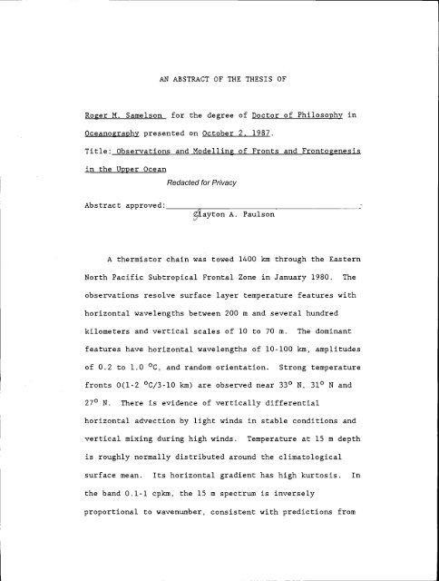
AN ABSTRACT OF THE THESIS OF<br />
Roger M. Samelson for the degree <strong>of</strong> Doctor <strong>of</strong> Philosophy in<br />
Oceanography presented on October 2. 1987.<br />
Title: <strong>Observations</strong> <strong>and</strong> <strong>Modelling</strong> <strong>of</strong> <strong>Fronts</strong> <strong>and</strong> <strong>Frontogenesis</strong><br />
in the Upper Ocean<br />
Abstract approved:<br />
Redacted for Privacy<br />
ayton A. Paulson<br />
A thermistor chain was towed 1400 km through the Eastern<br />
North Pacific Subtropical Frontal Zone in January 1980. The<br />
observations resolve surface layer temperature features with<br />
horizontal wavelengths between 200 m <strong>and</strong> several hundred<br />
kilometers <strong>and</strong> vertical scales <strong>of</strong> 10 to 70 m. The dominant<br />
features have horizontal wavelengths <strong>of</strong> 10-100 kin, amplitudes<br />
<strong>of</strong> 0.2 to 1.0 °C, <strong>and</strong> r<strong>and</strong>om orientation. Strong temperature<br />
fronts 0(1-2 °C/3-lO km) are observed near 330 N, 310 N <strong>and</strong><br />
270 N. There is evidence <strong>of</strong> vertically differential<br />
horizontal advection by light winds in stable conditions <strong>and</strong><br />
vertical mixing during high winds. Temperature at 15 m depth<br />
is roughly normally distributed around the climatological<br />
surface mean. Its horizontal gradient has high kurtosis. In<br />
the b<strong>and</strong> 0.1-1 cpkm, the 15 m spectrum is inversely<br />
proportional to wavenumber, consistent with predictions from
the theory <strong>of</strong> geostrophic turbulence, while the 70 m spectrum<br />
has additional variance consistent with Garrett-Munk internal<br />
wave displacements.<br />
We formulate analytically <strong>and</strong> solve numerically a<br />
semigeostrophic model for wind-driven thermocline upwelling.<br />
The model has a variable-density entraining mixed layer <strong>and</strong><br />
two homogeneous interior layers. All variables are uniform<br />
alongshore. A modified Ekman balance is prescribed far<br />
<strong>of</strong>fshore, <strong>and</strong> the normal-to-shore velocity field responds on<br />
the scales <strong>of</strong> the local internal deformation radii, which<br />
adjust dynamically. Sustained upwelling results in a step-<br />
like horizontal pr<strong>of</strong>ile <strong>of</strong> mixed layer density, as the layer<br />
interfaces "surface" <strong>and</strong> are advected <strong>of</strong>fshore. The upwelled<br />
horizontal pr<strong>of</strong>ile <strong>of</strong> mixed layer density scales with the<br />
initial internal deformation radii. Around the fronts,<br />
surface layer divergence occurs that is equal in magnitude to<br />
the divergence in the upwelling zone adjacent to the coast,<br />
but its depth penetration is inhibited by the stratification.
<strong>Observations</strong> <strong>and</strong> <strong>Modelling</strong> <strong>of</strong> <strong>Fronts</strong> <strong>and</strong> <strong>Frontogenesis</strong><br />
in the Upper Ocean<br />
by<br />
Roger M. Samelson<br />
A THESIS<br />
submitted to<br />
Oregon State University<br />
in partial fulfillment <strong>of</strong><br />
the requirements for the<br />
degree <strong>of</strong><br />
Doctor <strong>of</strong> Philosophy<br />
Completed October 2, 1987<br />
Commencement June 1988
APPROVED:<br />
Redacted for Privacy<br />
Pr<strong>of</strong>essqr <strong>of</strong> Oceanography in charge <strong>of</strong> major<br />
Redacted for Privacy<br />
Deane College <strong>of</strong> Oceanaphy<br />
Redacted for Privacy<br />
Dean <strong>of</strong> Graduth School<br />
Date thesis is presented October 2. 1987<br />
Typed by researcher for Roger M. Samelson
To my parents, Hans <strong>and</strong> Nancy Samelson
ACKNOWLEDGEMENTS<br />
I thank my advisor Clayton Paulson <strong>and</strong> the members <strong>of</strong> my<br />
committee for their support, guidance, <strong>and</strong> friendship.<br />
Clayton generously gave me the opportunity to explore a<br />
variety <strong>of</strong> projects. I owe him a debt <strong>of</strong> gratitude for his<br />
unwavering personal support. The first half <strong>of</strong> this thesis<br />
is based on his data; he guided me through its analysis.<br />
Rol<strong>and</strong> de Szoeke suggested the upwelling problem that makes<br />
up the second half <strong>of</strong> this thesis, <strong>and</strong> patiently guided me<br />
through it. John Allen invited my cooperation on a separate<br />
project. Doug Caidwell supported me during my first quarter.<br />
Rick Baumann's assistance during the analysis <strong>of</strong> the<br />
thermistor chain data went far beyond the call <strong>of</strong> duty. I am<br />
grateful to Jim Richman for conversations concerning the<br />
upwelling problem. Eric Beals <strong>and</strong> Steve Card provided<br />
comradeship in the trenches while the bits were flying.<br />
Erika Francis, John Lel<strong>and</strong>, Jeff Paduan <strong>and</strong> others kept me<br />
from going (entirely) <strong>of</strong>f the deep end. Harry Belier taught<br />
me much about the musical routes to chaos. I thank the<br />
scientists <strong>and</strong> crew <strong>of</strong> the R/V Wecoma, TH 87 Leg 2, for not<br />
throwing me to the sharks when they had the motive <strong>and</strong> the<br />
opportunity. Thanks to all those over the years who have<br />
helped me to appreciate that the ocean is more than an analog<br />
device for the solution <strong>of</strong> certain partial differential<br />
equations <strong>of</strong> mathematical physics.
This research was supported by ONR under contracts<br />
N00014-87-K-0009 <strong>and</strong> N00014-84-C-0218 <strong>and</strong> by NSF under grant<br />
OCE-8541635. Computations for Chapter III were carried out<br />
on the Cray-i at NCAR.
What in water did Bloom, waterlover, drawer <strong>of</strong><br />
water, watercarrier returning to the range, admire?<br />
Its universality. . . its vehicular ramifications<br />
in continental lakecontained streams <strong>and</strong> confluent<br />
oceanflowing rivers with their tributaries <strong>and</strong><br />
transoceanic currents: gulfstream, north <strong>and</strong> south<br />
equatorial courses: its violence in seaquakes,<br />
waterspouts, artesian wells, eruptions, torrents,<br />
eddies, freshets, spates, groundswells, watersheds,<br />
waterpartings, geysers, cataracts, whirlpools,<br />
maelstroms, inundations, deluges, cloudbursts: its<br />
vast circumterrestrial ahorizontal curve: its<br />
secrecy in springs.<br />
James Joyce, Ulysses<br />
Know ye, now, Bulkington? Glimpses do ye seem to<br />
see <strong>of</strong> that mortally intolerable truth; that all deep<br />
earnest thinking is but the intrepid effort <strong>of</strong> the soul<br />
to keep the open independence <strong>of</strong> her sea.. .?<br />
Herman Melville, Moby Dick<br />
Ver<strong>and</strong>ahs, where the pages <strong>of</strong> the sea<br />
are a book left open by an absent master<br />
in the middle <strong>of</strong> another life.<br />
Derek Walcott, Another Life
TABLE OF CONTENTS<br />
I. INTRODUCTION 1<br />
II. TOWED THERMISTOR CHAIN OBSERVATIONS OF UPPER<br />
OCEAN FRONTS IN THE SUBTROPICAL NORTH PACIFIC 3<br />
Abstract 3<br />
11.1 Introduction 4<br />
11.2 Instrumentation <strong>and</strong> data collection 6<br />
11.3 <strong>Observations</strong> 8<br />
11.4 Analysis 14<br />
II.4.a Statistics 14<br />
II.4.b Spectra 16<br />
11.5 Geostrophic turbulence 21<br />
11.6 Summary 26<br />
11.7 References 44<br />
III. SEMIGEOSTROPHIC WIND-DRIVEN THERMOCLINE UPWELLING<br />
AT A COASTAL BOUNDARY 46<br />
Abstract 46<br />
111.1 Introduction 47<br />
111.2 Model formulation 49<br />
III.2.a Equations 49<br />
III.2.b Matching conditions 56<br />
III.2.c Nondimensionalization 60<br />
III.2.d Outline <strong>of</strong> numerical method 62<br />
111.3 Thermocline upwelling: numerical results<br />
<strong>and</strong> discussion 65<br />
111.4 Summary 72<br />
111.5 References 82<br />
BIBLIOGRAPHY 83<br />
APPENDIX A: DYNAMICAL DERIVATION OF A MATCHING CONDITION 86<br />
APPENDIX B: NIJMERICAL METHOD 89
LIST OF FIGURES<br />
Fizure Page<br />
11.1 Tow tracks 29<br />
11.2 Hourly sea surface temperature vs. salinity<br />
from on-board CTD during 16-28 Jan., with<br />
contours <strong>of</strong> 30<br />
11.3 Hourly sea surface temperature, salinity <strong>and</strong><br />
from on-board CTD vs. latitude 31<br />
t<br />
11.4 Nominal 15 m (solid) <strong>and</strong> 70 m (dashed)<br />
thermistor temperature (horizontal 500 m<br />
means) vs. distance along tow tracks 32<br />
11.5 Examples <strong>of</strong> fronts shown by isotherm crosssections<br />
(interpolated from horizontal 100 m<br />
mean thermistor temperatures) vs. depth <strong>and</strong><br />
distance along tow tracks 33<br />
11.6 Probability density <strong>of</strong> difference <strong>of</strong> 15 m<br />
temperature from climatological surface<br />
temperature 34<br />
11.7 Probability density <strong>of</strong> 15 m horizontal<br />
temperature gradient 35<br />
11.8 Horizontal wavenuniber spectrum <strong>of</strong> horizontal<br />
temperature gradient from Tows 1, 2a, 2b, 3a,<br />
<strong>and</strong> 4, ensemble averaged <strong>and</strong> b<strong>and</strong> averaged<br />
to 5 b<strong>and</strong>s per decade 36<br />
11.9 Horizontal wavenuniber spectra <strong>of</strong> horizontal<br />
temperature gradient from Tows 1, 2a, 2b, 3a,<br />
<strong>and</strong> 4, b<strong>and</strong> averaged to 10 b<strong>and</strong>s per decade 37<br />
11.10 Horizontal wavenumber spectra <strong>of</strong> 15 m <strong>and</strong> 70 m<br />
temperature for Tows 1, 2a, 2b, 3a, <strong>and</strong> 4,<br />
ensemble averaged <strong>and</strong> b<strong>and</strong> averaged to 5<br />
b<strong>and</strong>s per decade 38<br />
11.11 Estimated 70 m internal wave vertical<br />
displacement spectra from difference <strong>of</strong> 70 m<br />
<strong>and</strong> 15 m power spectra, b<strong>and</strong> averaged to 10<br />
b<strong>and</strong>s per decade (solid lines: x -- Tow 2a,<br />
+ Tow 2b, X -- Tow 4) 39
Figure<br />
LIST OF FIGURES (continued)<br />
Page<br />
11.12 Horizontal wavenuniber spectra <strong>and</strong> coherence,<br />
ensemble averaged <strong>and</strong> b<strong>and</strong> averaged to 5 b<strong>and</strong>s<br />
per decade 40<br />
111.1 Model geometry 77<br />
111.2 Nondimensional mixed layer density, layer<br />
depths, <strong>and</strong> normal-to-shore transport vs.<br />
<strong>of</strong>fshore distance at times t/t* = 8.1 (a-c),<br />
16.0 (d-f), 21.0 (g-i), 25.4 (j-l) 78<br />
111.3 Nondiinensional alongshore geostrophic<br />
velocities at time t/t* 25.4 79<br />
111.4 Nondimensional positions <strong>of</strong> fronts' vs. time<br />
for Cases 1 (a), 2 (b), <strong>and</strong> 3 (c) 80<br />
111.5 Nondimensional characteristic curves vs. time<br />
for Case 1 in layers 1 (a), 2 (b), <strong>and</strong> 3 (c) 81
LIST OF TABLES<br />
Table Page<br />
11.1 Tow start <strong>and</strong> finish positions <strong>and</strong> times 41<br />
11.2 Winds <strong>and</strong> surface fluxes 42<br />
11.3 Climatological sea surface temperature (°C),<br />
averaged over 150-155° W 43
OBSERVATIONS AND MODELLING OF FRONTS AND FRONTOGENESIS<br />
IN THE UPPER OCEAN<br />
I. INTRODUCTION<br />
This thesis comprises two separate projects. The common<br />
theme is fronts <strong>and</strong> frontogenesis in the upper ocean.<br />
<strong>Fronts</strong>, regions <strong>of</strong> unusually large horizontal gradients<br />
in fluid properties, are an important form <strong>of</strong> physical<br />
oceanographic variability. Though they have received<br />
considerable attention from oceanographers (the recent<br />
monograph The Physical Nature <strong>and</strong> Structure <strong>of</strong> Oceanic <strong>Fronts</strong><br />
(Fedorov, 1986) contains 279 references), a full<br />
underst<strong>and</strong>ing <strong>of</strong> their role in the ocean still awaits us.<br />
In Chapter II, we present an analysis <strong>of</strong> upper ocean<br />
temperature data collected near the North Pacific Subtropical<br />
Frontal Zone. In this region <strong>of</strong> the North Pacific, the<br />
large-scale meridional gradients <strong>of</strong> temperature, salinity,<br />
<strong>and</strong> density are intensified in a Frontal Zone. Wind-driven<br />
convergence is the probable primary cause <strong>of</strong> this<br />
intensification (Roden, 1975). Many small scale fronts are<br />
evident in the data. Baroclinic instability is likely<br />
important in the development <strong>of</strong> these smaller scale features.<br />
In Chapter III, we present a model for wind-driven<br />
therniocline upwelling at a coastal boundary. In this case,<br />
the action <strong>of</strong> the wind on the ocean is again frontogenetic.
Here, however, a divergence drives the frontogenesis, as<br />
fluid is drawn up at the boundary to produce horizontal<br />
gradients from vertical stratification.<br />
The basic physics <strong>of</strong> the upwelling process analyzed in<br />
Chapter III should essentially apply (with appropriate<br />
rescaling <strong>and</strong> some additional dynamics) to wind-driven<br />
upwelling in the Subarctic gyre north <strong>of</strong> the Subtropical<br />
Frontal Zone. Since the meridional gradient in surface layer<br />
properties may be partially maintained by this upwelling,<br />
further investigations may eventually link the ideas <strong>and</strong><br />
observations <strong>of</strong> these two Chapters in an unexpected <strong>and</strong><br />
relatively direct manner.<br />
2
II. TOWED THERMISTOR CHAIN OBSERVATIONS OF FRONTS<br />
IN THE SUBTROPICAL NORTH PACIFIC<br />
Abstract<br />
A thermistor chain was towed 1400 km through the Eastern<br />
North Pacific Subtropical Frontal Zone in January 1980. The<br />
observations resolve surface layer temperature features with<br />
horizontal wavelengths between 200 m <strong>and</strong> several hundred<br />
kilometers <strong>and</strong> vertical scales <strong>of</strong> 10 to 70 m. The dominant<br />
features have horizontal wavelengths <strong>of</strong> 10-100 km, amplitudes<br />
<strong>of</strong> 0.2 to 1.0 °C, <strong>and</strong> r<strong>and</strong>om orientation. Associated with<br />
them is a plateau below 0.1 cpkm in the horizontal<br />
temperature gradient spectrum that is coherent between 15 <strong>and</strong><br />
70 m depths. They likely arise from baroclinic instability.<br />
Strong temperature fronts 0(1-2 °C/3-10 km) are observed near<br />
330 N, 31° N <strong>and</strong> 27° N. Temperature variability is partially<br />
density compensated by salinity, with the fraction <strong>of</strong><br />
compensation increasing northward. There is evidence <strong>of</strong><br />
vertically differential horizontal advection by light winds<br />
in stable conditions, vertical mixing during high winds, <strong>and</strong><br />
shallow convection caused by wind-driven advection <strong>of</strong> denser<br />
water over less dense water. Temperature at 15 m depth is<br />
roughly normally distributed around the climatological<br />
surface mean, with a st<strong>and</strong>ard deviation <strong>of</strong> approximately 0.7<br />
°C, while its horizontal gradient has high kurtosis <strong>and</strong><br />
3
maximum values in excess <strong>of</strong> 0.25 °C/l00 m. In the b<strong>and</strong> 0.1-1<br />
cpkm, the 15 m spectrum is very nearly inversely proportional<br />
to wavenumber, consistent with predictions from geostrophic<br />
turbulence theory, while the spectrum at 70 m depth has<br />
additional variance that is consistent with Garrett-Munk<br />
internal wave displacements.<br />
11.1 Introduction<br />
The North Pacific Subtropical Frontal Zone is a b<strong>and</strong> <strong>of</strong><br />
relatively large mean meridional upper ocean temperature <strong>and</strong><br />
salinity gradient centered near 30° N (Roden, 1973). Its<br />
existence is generally attributed to wind-driven surface<br />
convergence <strong>and</strong> large-scale variations in air-sea heat <strong>and</strong><br />
water fluxes (Roden, 1975). A recent attempt has been made<br />
to determine the associated large-scale geostrophic flow<br />
(Niiler <strong>and</strong> Reynolds, 1984), <strong>and</strong> hydrographic surveys (Roden,<br />
1981) <strong>of</strong> the Subtropical Frontal Zone have revealed energetic<br />
mesoscale eddy fields. However, little is known about the<br />
dynamics <strong>of</strong> the local mesoscale circulation or the detailed<br />
structure, generation, <strong>and</strong> dissipation <strong>of</strong> individual frontal<br />
features.<br />
Here we report on an investigation <strong>of</strong> the upper ocean<br />
thermal structure <strong>of</strong> fronts in the North Pacific Subtropical<br />
Frontal Zone. We use the term "Frontal Zone" rather than<br />
"Front" because these wintertime measurements show r<strong>and</strong>omly<br />
4
oriented multiple surface fronts up to 2 °C in magnitude <strong>and</strong><br />
less than 10 km in width. <strong>Observations</strong> were made in January<br />
1980 with a towed thermistor chain that measured temperature<br />
at 12 to 21 depths in the upper 100 m <strong>of</strong> the water column.<br />
The thermistor chain was towed a distance <strong>of</strong> 1400 km in an<br />
area <strong>of</strong> the Pacific bounded by 26° <strong>and</strong> 340 N, 1500 <strong>and</strong> 158°<br />
W. The observations resolve surface layer temperature<br />
features with horizontal wavelengths between 200 m <strong>and</strong><br />
several hundred km <strong>and</strong> vertical scales <strong>of</strong> 10 to 70 m. The<br />
towed thermistor chain <strong>and</strong> data collection procedure are<br />
described in Section 11.2. Section 11.3 is devoted to a<br />
description <strong>of</strong> the fronts, their magnitude <strong>and</strong> horizontal<br />
scales, temperature-salinity compensation, vertical<br />
stratification, <strong>and</strong> response to wind. Probability densities<br />
<strong>of</strong> surface (15 m) temperature (with the climatological mean<br />
removed) <strong>and</strong> surface temperature gradient are presented in<br />
Section II.4.a. Horizontal wavenumber spectra <strong>of</strong> temperature<br />
<strong>and</strong> temperature gradient at several depths between 15 <strong>and</strong> 70<br />
m are presented in Section II.4.b. In Section 11.5, the high<br />
wavenumber tail <strong>of</strong> the temperature spectrum is compared with<br />
the predictions <strong>of</strong> the theory <strong>of</strong> geostrophic turbulence<br />
(Charney, 1971). Section 11.6 contains a summary.<br />
5
11.2 Instrumentation <strong>and</strong> data collection<br />
The thermistor chain tows were made during FRONTS 80, a<br />
multi-investigator endeavor focused on the Subtropical<br />
Frontal Zone near 310 N, 155° W, in January 1980. Other<br />
measurements by other investigators included CTD surveys<br />
(Roden, 1981), remotely sensed infrared radiation (Van<br />
Woert, 1982), XCP velocity pr<strong>of</strong>iles (Kunze <strong>and</strong> Sanford,<br />
1984), <strong>and</strong> drifting buoy tracks (Niiler <strong>and</strong> Reynolds, 1984).<br />
The thermistor chain has been described in Paulson et<br />
(1980). The chain was 120 m long, with a 450 kg lead<br />
depressor to maintain a near vertical alignment while it was<br />
towed behind the ship. Sensors were located at approximately<br />
4 m intervals over the lower 82 m. These sensors included 27<br />
Thermometrics P-85 thermistors <strong>and</strong> three pressure<br />
transducers. The thermistors have a response time <strong>of</strong> 0.1 s,<br />
relative accuracy <strong>of</strong> better than iO3 °C, <strong>and</strong> absolute<br />
accuracy <strong>of</strong> roughly 10-2 °C. Data were recorded at a<br />
sampling frequency <strong>of</strong> 10 Hz. For this analysis, individual<br />
thermistor data records were averaged to values at 100 m<br />
intervals using ship speed from two-hourly positions<br />
interpolated from satellite fixes. Since this speed varied<br />
(from 2 to 6 m s1-), the averaged values contain a variable<br />
number <strong>of</strong> data points (from 166 to 502). The averaging<br />
removes the effects <strong>of</strong> ship roll <strong>and</strong> pitch <strong>and</strong> surface
gravity waves. A maximum <strong>of</strong> 21 <strong>and</strong> a minimum <strong>of</strong> 12<br />
thermistors functioned for entire tows. Thermistor depths<br />
were obtained from the ship's log speed <strong>and</strong> a model <strong>of</strong> the<br />
towed chain configuration calibrated by data from the<br />
pressure transducers. Temperature measurements were obtained<br />
at maximum <strong>and</strong> minimum depths <strong>of</strong> 95 m <strong>and</strong> 4 m.<br />
The tow tracks are displayed in Figure 11.1. The four<br />
tows are labeled by number in chronological order. Since the<br />
tracks for Tows 2 <strong>and</strong> 3 overlap, the track for Tow 3, which<br />
took place on 25 January, is displayed separately, overlaid<br />
on a contour <strong>of</strong> temperature at 20 m from the Roden CTD survey<br />
during 24-30 January. Tows 2 <strong>and</strong> 3 are each divided into<br />
sections, labeled a <strong>and</strong> b, by course changes. The tow start<br />
<strong>and</strong> finish positions <strong>and</strong> times are given in Table 11.1.<br />
During 19-26 January, the ship remained within the rectangle<br />
indicated by dashed lines in Figure 11.1.<br />
Surface salinity was determined from temperature <strong>and</strong><br />
conductivity measured by a Bisset Berman CTD located in the<br />
ship's wet lab, to which water was pumped from a sea chest at<br />
approximately 5 m depth. The cycle time for the fluid in<br />
this system was roughly 5-10 minutes during most <strong>of</strong> the<br />
experiment. The CTD temperature, corrected for<br />
(approximately 1 °C) intake warming by comparison with data<br />
from the uppermost thermistor, was used to obtain surface<br />
density. CTD conductivity <strong>and</strong> temperature were recorded<br />
7
hourly (once every 10-20 km at typical tow speeds), as were<br />
surface wind speed <strong>and</strong> direction (from an anemometer at 34.4<br />
m height), dry <strong>and</strong> wet bulb air temperatures, <strong>and</strong> incident<br />
solar radiation.<br />
11.3 <strong>Observations</strong><br />
Sea surface temperature <strong>and</strong> salinity from ship-board CTD<br />
measurements during 16-28 January are displayed with contours<br />
<strong>of</strong> at (density) in Figure 11.2. The data range over 7 °C in<br />
temperature (T) <strong>and</strong> 1 ppt in salinity (S). Though<br />
temperature may vary by 1 °C at constant salinity, most <strong>of</strong><br />
the data approximately obey a single identifiable T-S<br />
relation, with the exception <strong>of</strong> four points with T > 20.5 °C,<br />
S . 35.1<br />
ppt, which occurred after the encounter <strong>of</strong> a strong<br />
front at the southern end <strong>of</strong> Tow 4. Salinity tends to<br />
compensate temperature, so the density variations are small,<br />
but relative temperature still tends to indicate relative<br />
density (warmer, more saline, water is typically less dense).<br />
Surface temperature, salinity, <strong>and</strong> at are displayed<br />
versus latitude in Figure 11.3. Scales have been chosen<br />
using the equation <strong>of</strong> state so that a unit distance change in<br />
temperature (salinity) at constant salinity (temperature)<br />
corresponds approximately to a unit distance change in at.<br />
Temperature <strong>and</strong> salinity tend to decrease toward higher<br />
latitudes. The corresponding density gradient is relatively
small, since the large-scale temperature <strong>and</strong> salinity<br />
gradients are density-compensating. Features with smaller<br />
horizontal scales also show compensation. A front near 300 N<br />
was crossed several times during 19-27 January <strong>and</strong> appears as<br />
a noisy step-like, partially compensated, feature. (Its<br />
apparent sharpness is exaggerated by a set <strong>of</strong> measurements<br />
taken during frontal transects at constant latitude.) The<br />
large temperature feature near 330 N is roughly 70%<br />
compensated by salinity. In contrast, the 2 °C front near<br />
27° N has negligible salinity variation. There appears to be<br />
a density feature with roughly 300 km wavelength between 310<br />
N <strong>and</strong> 34° N.<br />
For each <strong>of</strong> the tows, Figure 11.4 displays traces <strong>of</strong> 500<br />
m horizontal averages <strong>of</strong> nominal 15 m (solid line) <strong>and</strong> 70 m<br />
(dashed line) thermistor temperature. These are respectively<br />
the shallowest <strong>and</strong> deepest depths at which thermistor<br />
measurements were made during all four tows. The dominant<br />
temperature features have horizontal wavelengths <strong>of</strong> 10 to 100<br />
km, amplitudes <strong>of</strong> 0.2 to 1.0 °C, <strong>and</strong> no apparent preferred<br />
orientation with respect to the large-scale (climatological)<br />
temperature gradient. Satellite imagery <strong>of</strong> the Subtropical<br />
Frontal Zone in January <strong>and</strong> February 1980 (Van Woert, 1981,<br />
1982), some <strong>of</strong> which is precisely simultaneous with the tows,<br />
shows a sea surface temperature field composed <strong>of</strong> highly<br />
distorted isotherms, such as result from advection <strong>of</strong> a
tracer by a strain field, rather than a collection <strong>of</strong><br />
isolated patches <strong>of</strong> r<strong>and</strong>om temperature. The thermistor chain<br />
tows are cross-sections <strong>of</strong> this field. On horizontal scales<br />
<strong>of</strong> hundreds <strong>of</strong> kilometers, several large fronts, across which<br />
the temperature change (roughly 1 °C or more) has the same<br />
sign as the large-scale gradient, give a step-like appearance<br />
to the temperature record.<br />
The salinity-compensated temperature structure that<br />
dominates Tow 1 is visible near 33° N in Figure 11.3.<br />
Measured horizontal temperature gradients exceeded 0.25<br />
°C/lOOm in the front near 110 km, the largest observed during<br />
the experiment.<br />
In Tow 2a, a large front was encountered at 200 km, near<br />
300 N. The feature in Tow 2b near 70 km appears to be a<br />
me<strong>and</strong>er <strong>of</strong> the same front. This me<strong>and</strong>er is visible in<br />
infrared satellite imagery from 17 January 1980 (Figure 2a,<br />
Van Woert, 1982).<br />
Tow 3, made on 25 January, was contained in the region<br />
covered by a CTD survey (Roden, 1981) during 24-31 January.<br />
The tow is roughly perpendicular to the isotherms <strong>of</strong> the<br />
surveyed front (Figure II.lb). The mean temperature gradient<br />
is large over this entire tow. The sharp frontal boundary<br />
near 18 °C observed a week earlier at the same location<br />
during Tow 2a, does not appear in Tow 3. A tongue <strong>of</strong> warm<br />
water was crossed at the southern end <strong>of</strong> the tow, with a<br />
10
front at about 18.5 °C. There is frontal structure near 60<br />
kin, at about 17.5 0C, in both Tows 3a <strong>and</strong> 3b. Note the<br />
similarity <strong>of</strong> Tows 3a <strong>and</strong> 3b, which were made on the same<br />
track (in opposing directions) but several hours apart.<br />
The largest temperature front encountered during the<br />
experiment, with horizontal gradient reaching 1.5 °C/3 km <strong>and</strong><br />
a temperature change <strong>of</strong> roughly 2 °C over 10 kin, occurred<br />
near 27° N at 350 km in Tow 4. The salinity change across<br />
this feature is small <strong>and</strong> in fact enhances the density<br />
change, which is approximately 0.5 kg m3 over 10 km, most <strong>of</strong><br />
it occurring over 3 km. This is larger than the density<br />
variability observed over the entire remainder <strong>of</strong> the<br />
experiment. Isotherm cross-sections <strong>of</strong> this front are shown<br />
in Figure II.5a. The geostrophic vertical shear across the<br />
front is roughly 10-2 s- at the surface. Large amplitude<br />
internal wave vertical displacements <strong>of</strong> the seasonal<br />
thermocline are visible.<br />
The vertical temperature gradient between 15 m <strong>and</strong> 70 m<br />
was generally weak except in regions near frontal features.<br />
During Tow 1, appreciable vertical gradients appear only<br />
within 10-15 km <strong>of</strong> the fronts. During Tow 2, some vertical<br />
gradients occur up to 25-30 km from fronts (though there may<br />
be closer fronts that lie <strong>of</strong>f the tow track). The upper 70 m<br />
are nearly homogeneous in temperature over most <strong>of</strong> Tow 3a. A<br />
small amount <strong>of</strong> stratification is evident near features<br />
11
etween 50 <strong>and</strong> 75 km <strong>and</strong> in the warm tongue near 110 km.<br />
These features <strong>and</strong> the associated vertical gradients are<br />
evident as well in Tow 3b, which followed the same track on<br />
the opposite course. In Tow 4, as in Tows 1 <strong>and</strong> 2, vertical<br />
gradients are found consistently near frontal features.<br />
Often the upper sections <strong>of</strong> individual fronts appear<br />
displaced horizontally by several kilometers from the lower<br />
sections. During Tow 2, particularly over the interval<br />
125-300 km, 15 m temperatures have traces that are similar to<br />
the 70 in temperatures but <strong>of</strong>fset to the north. Winds (Table<br />
11.2) during 17 January were from the south, <strong>and</strong> may have<br />
displaced a shallow layer northward <strong>and</strong> eastward. Isotherm<br />
cross-sections <strong>of</strong> the feature near 135 kin are shown in Figure<br />
II.5b. (Note that the presence <strong>of</strong> a temperature inversion<br />
implies an anomalous local T-S relation, according to which<br />
the warmer, more saline water is denser.) The displacement<br />
can only be estimated, since the angle <strong>of</strong> incidence <strong>of</strong> the<br />
tow track across the front is unknown, but it appears to be a<br />
few kilometers. This is an appropriate value for Ekman layer<br />
flow in response to light winds whose direction varies on a<br />
2-5 day time scale, <strong>and</strong> is typical <strong>of</strong> such features in the<br />
data, most <strong>of</strong> which occurred after periods <strong>of</strong> light winds.<br />
Estimates <strong>of</strong> daily average buoyancy flux, made from hourly<br />
bulk estimates <strong>of</strong> surface fluxes, are shown in Table 2, <strong>and</strong><br />
Monin-Obukhov depths calculated from the flux estimates are<br />
12
given in the stable cases (downward buoyancy flux). The<br />
uncertainty in the flux estimates is roughly 20%. The<br />
Monin-Obukhov depth for 17 January, the date <strong>of</strong> the<br />
observations shown in Figure II.5b, is 62 m. This is<br />
comparable to the depth <strong>of</strong> the displaced upper section.<br />
Convection in the mixed layer may have prevented a similar<br />
structure from forming as wind stress forced denser fluid<br />
over less dense fluid at the right-h<strong>and</strong> front in Figure 5b.<br />
Vertical gradients in the surface layer are negligible<br />
over the last 70 kin <strong>of</strong> Tow 2 in spite <strong>of</strong> horizontal gradients<br />
as large as those over the first 540 km. During this last<br />
period <strong>of</strong> Tow 2b, local wind speeds rose from 5-10 m s to<br />
20 m sfl-, where they remained until after the tow was<br />
terminated. (Table 11.2 gives daily vector averaged hourly<br />
winds; daily average magnitudes are larger.) The surface<br />
layer is nearly uniform in temperature to 70 m depth over<br />
most <strong>of</strong> Tow 3 as well. Maximum wind speeds <strong>of</strong> 20 m s were<br />
attained in this region two days prior to Tow 3. The absence<br />
<strong>of</strong> vertical gradients during these two periods is likely due<br />
to vertical mixing in response to the high winds. Tow 3 was<br />
taken along part <strong>of</strong> the line covered by Tow 2a <strong>and</strong> runs<br />
between the locations <strong>of</strong> hydrographic stations occupied by<br />
the CTD survey (Roden, 1981). The surface temperature in<br />
this region decreased by approximately 1 °C between Tows 2a<br />
<strong>and</strong> 3. Roden (1981) interprets this decrease as southward<br />
13
advection <strong>of</strong> a tongue <strong>of</strong> cold water in a frontal me<strong>and</strong>er, but<br />
cooling by entrainment may also have contributed. Large<br />
(1986) present evidence for large entrainment events in<br />
the North Pacific during the fall season. These appear to be<br />
shear mixing events driven by the near-inertial response to<br />
storms.<br />
A 0.7 °C temperature inversion, roughly 5 kin wide,<br />
occurred at 100 kin, near the well-compensated front<br />
encountered during Tow 1. Isotherm cross-sections <strong>of</strong> this<br />
feature are displayed in Figure II,5c. The presence <strong>of</strong> an<br />
inversion implies an anomalous local T-S relation, according<br />
to which the warmer, more saline water is denser. The warm,<br />
dense water most likely originated from the warm side <strong>of</strong> the<br />
front, with which it may be contiguous. The wind record<br />
(Table 11.2) suggests an Ekman flow to the southeast, nearly<br />
normal to the tow track, so that the cooler surface water may<br />
have been advected over the warmer water from the northwest.<br />
II.4.a Statistics<br />
11.4 Analysis<br />
To characterize the temperature variability<br />
statistically, we have calculated probability densities <strong>of</strong><br />
temperature gradient <strong>and</strong> temperature deviation from<br />
climatology. Table 11.3 lists climatological surface<br />
14
temperatures for January <strong>and</strong> February from 100 years <strong>of</strong> ship<br />
observations <strong>and</strong> 27 years <strong>of</strong> hydrocasts (Robinson, 1976).<br />
Figure 11.6 shows the probability density <strong>of</strong> the deviation <strong>of</strong><br />
15 m temperatures from a fit, linear in latitude in the<br />
intervals 253O0 N <strong>and</strong> 30-35° N, to the January climatology.<br />
As noted by Roden (1981), the surface layer temperatures are<br />
colder on average than the climatological means. The<br />
apparent bimodality is probably due to poor statistics. The<br />
st<strong>and</strong>ard deviation is roughly 0.5 °C. Relative to the<br />
climatological gradient, this would correspond to an<br />
adiabatic meridional displacement <strong>of</strong> 80-100 km. From<br />
drifters deployed near 30° N, 150° W, Niiler <strong>and</strong> Reynolds<br />
(1984) compute a mean northward surface velocity <strong>of</strong> 1-2 cm<br />
s1- during 27 January through 30 April 1980. From infrared<br />
imagery, Van Woert (1982) estimates an e-folding time <strong>of</strong> 60<br />
days for a large frontal me<strong>and</strong>er near 30 N during January <strong>and</strong><br />
February 1980. The meridional displacement scale is<br />
comparable to the product <strong>of</strong> these velocity <strong>and</strong> time scales.<br />
St<strong>and</strong>ard mixing-length arguments yield an eddy diffusivity<br />
(as velocity times length or length squared divided by time)<br />
<strong>of</strong> 1-2 x l0 m2 s1-. This is an order <strong>of</strong> magnitude smaller<br />
than typical values used in numerical models (e.g., Lativ,<br />
1987)<br />
Horizontal 100 m mean temperature gradients were<br />
calculated from differences <strong>of</strong> adjacent 15 m temperatures.<br />
15
Figure 11.7 displays the probability density <strong>of</strong> these<br />
gradients. The dotted line represents a Gaussian<br />
distribution with the observed mean <strong>and</strong> st<strong>and</strong>ard deviation.<br />
The observed kurtosis is 76, much larger than the Gaussian<br />
value <strong>of</strong> 3. This suggests the presence <strong>of</strong> a velocity field<br />
that strains the temperature gradients to small scales. The<br />
large kurtosis is characteristic <strong>of</strong> processes with sharp<br />
transitions between small <strong>and</strong> large values. It measures the<br />
front-like nature <strong>of</strong> the surface temperature field, which is<br />
dominated by intermittent large gradients separated by<br />
regions <strong>of</strong> small gradients. Qualitatively similar<br />
distributions <strong>of</strong> temperature <strong>and</strong> velocity gradients occur at<br />
small scales in three-dimensional turbulence (Monin <strong>and</strong><br />
Yaglom, 1975). Calculations <strong>of</strong> the kurtosis for<br />
distributions <strong>of</strong> average horizontal gradient over distances<br />
from 100 m to 100 km show that the kurtosis increases sharply<br />
below scales <strong>of</strong> 10 km, with an evident but irregular change<br />
in dependence at a few hundred meters, roughly the vertical<br />
scales <strong>of</strong> the surface boundary layer.<br />
II.4.b Spectra<br />
Figure 11.8 displays the ensemble averaged horizontal<br />
wavenumber spectrum <strong>of</strong> 15 m horizontal temperature gradient,<br />
b<strong>and</strong> averaged to 5 b<strong>and</strong>s per decade. The variability between<br />
10 <strong>and</strong> 100 km wavelengths that is evident in the time series<br />
16
dominates the spectrum. At these wavenumbers <strong>and</strong> at<br />
wavenumbers above 1 cpkm, the spectrum is approximately<br />
constant. Between 0.1 cpkm <strong>and</strong> 1 cpkm, the spectrum is very<br />
nearly proportional to k1-, where k is wavenumber.<br />
We associate the low wavenumber plateau with the<br />
mesoscale eddy field, the likely source <strong>of</strong> the dominant<br />
temperature features. The constant spectral level is a<br />
typical signature <strong>of</strong> an eddy production range, which may be<br />
driven by baroclinic instability. This instability generally<br />
prefers the scale <strong>of</strong> the internal deformation radius. The<br />
first local internal deformation radius, calculated using a<br />
FRONTS 80 CTD station for the upper 1500 m supplemented by<br />
deep data from a 1984 meridional transect, is 40 km, which<br />
lies within the energetic plateau, toward its less resolved<br />
low wavenumber end. The break in slope at the high<br />
wavenumber end <strong>of</strong> the plateau occurs near 0.1 cpkm, at<br />
roughly the fifth internal deformation radius. The constant<br />
spectral level at wavenumbers above 1 cpkm is likely due to<br />
temperature gradient production in the surface boundary<br />
layer.<br />
Figure 11.9 displays horizontal wavenumber spectra <strong>of</strong> 15<br />
m horizontal temperature gradient from each individual tow,<br />
b<strong>and</strong> averaged to 10 b<strong>and</strong>s per decade. The spectral levels<br />
vary by roughly half a decade. The spectral shapes are<br />
nearly uniform, despite the apparent difference in the<br />
17
qualitative nature <strong>of</strong> the records noted in Section 11.3<br />
(e.g., the single large feature in Tow 1 versus the myriad<br />
smaller features in Tows 2a, 2b). Each spectrum has a broad<br />
peak or plateau at low wavenumber, a break in slope near 10<br />
km, <strong>and</strong> is approximately proportional to k1- between 10 km<br />
<strong>and</strong> 1 km. A minimum occurs between 1 km <strong>and</strong> 350 m<br />
wavelengths in three <strong>of</strong> the five spectra. A secondary peak<br />
appears near 350 m in these three spectra, followed by a<br />
decrease toward the Nyquist wavelength (200 m). The spectra<br />
appear to fall <strong>of</strong>f slightly toward wavelengths larger than 50<br />
km. In this region however the number <strong>of</strong> data points is<br />
small <strong>and</strong> the 95% confidence intervals large. The spectrum<br />
from Tow 3b is not shown. At the 95% confidence level, it is<br />
essentially indistinguishable from the Tow 3a spectrum.<br />
Because <strong>of</strong> the close time <strong>and</strong> space scales, we interpret this<br />
as a lack <strong>of</strong> independence between the two spectral estimates<br />
from Tow 3, <strong>and</strong> have only included the estimate from Tow 3a<br />
in the ensemble average.<br />
Figure 11.10 displays ensemble averaged horizontal<br />
wavenumber spectra <strong>of</strong> 15 m <strong>and</strong> 70 m temperature, b<strong>and</strong><br />
averaged to 5 b<strong>and</strong>s per decade. We interpret the difference<br />
between the spectral levels at 15 m <strong>and</strong> 70 m in the b<strong>and</strong>s<br />
above 0.1 cpkm as internal wave vertical displacements at 70<br />
m. Since the average vertical temperature gradients are<br />
small at 15 m (less than l0 0C ma-; at 70 m they are<br />
18
typically iO-2iO3 °c m1-), <strong>and</strong> since the vertical internal<br />
wave velocities must vanish at the surface, temperature<br />
variance from internal wave isotherm displacements will be<br />
small at 15 m. If the 70 m spectrum is composed <strong>of</strong> the sum<br />
<strong>of</strong> an internal wave vertical displacement spectrum that is<br />
uncorrelated with the 15 m spectrum <strong>and</strong> a spectrum (due to<br />
other processes) equal in variance to the 15 m spectrum at<br />
each wavenumber, the 70 m internal wave spectrum will be the<br />
difference <strong>of</strong> the power spectra at 70 m <strong>and</strong> 15 m.<br />
(Differencing the series leads to an overestimate <strong>of</strong> the<br />
internal wave variance, as incoherent parts not due to<br />
internal waves will contribute to the power spectrum <strong>of</strong> the<br />
differenced series.) Using average vertical temperature<br />
gradients at 70 m from entire tow means <strong>of</strong> surrounding<br />
thermistors to estimate displacements <strong>and</strong> the local buoyancy<br />
frequency, we obtain for Tows 2 <strong>and</strong> 4 the internal wave<br />
energy spectral estimates shown in Figure 11.11. The<br />
empirical Garrett-Munk prediction (Eq. Al2, Katz <strong>and</strong> Briscoe,<br />
1979; Garrett <strong>and</strong> Munk, 1972), with Desaubies (1976)<br />
parameters r 320 m2 h1- <strong>and</strong> t = 4 x l0 cph cpm-, is<br />
plotted for comparison. The spectral levels are mostly<br />
within 2 to 3 times the predicted values, <strong>and</strong> the spectral<br />
slopes show excellent agreement. A large temperature<br />
inversion <strong>and</strong> small vertical gradients prevented reliable<br />
calculations for Tows 1 <strong>and</strong> 3. Even in Tows 2 <strong>and</strong> 4, average<br />
19
temperature differences <strong>of</strong> surrounding thermistors are not<br />
far from the noise level <strong>of</strong> the calibrations, so these<br />
estimates have limited value as measurements <strong>of</strong> internal wave<br />
energy. They are however consistent with the assumption that<br />
the difference in the 70 m <strong>and</strong> 15 m spectral levels in the<br />
0.1-1 cpkm b<strong>and</strong> is due to internal waves, <strong>and</strong> that the<br />
variance in the 15 m spectrum in this b<strong>and</strong> is due to other<br />
processes. Below 0.1 cpkm, where the break in slope in the<br />
15 m spectrum occurs, the internal wave energy appears to<br />
fall <strong>of</strong>f. This apparently fortuitous correspondence gives<br />
the 70 m spectrum a nearly uniform slope (Figure 11.10).<br />
Figure 11.12 displays ensemble averaged spectra <strong>of</strong><br />
horizontal temperature gradients at 15, 23, 31, 50, <strong>and</strong> 70 m,<br />
as well as ensemble averaged coherence from cross-spectra<br />
between the 15 m record <strong>and</strong> the others, all b<strong>and</strong> averaged to<br />
5 b<strong>and</strong>s per decade. There is significant vertical coherence<br />
in the 0.1-1 cpkm b<strong>and</strong> over most <strong>of</strong> the surface layer. Where<br />
the internal wave variance raises the spectral levels above<br />
the 15 m values, coherence is rapidly destroyed. This occurs<br />
at successively shorter wavelengths as the vertical<br />
separation decreases, presumably since only short wavelength<br />
internal waves may exist on infrequent shallow patches <strong>of</strong><br />
vertical gradient.<br />
20
11.5 Geostrophic turbulence<br />
We have interpreted the low wavenumber plateau in the 15<br />
m horizontal temperature gradient spectrum (Figure 11.8) as<br />
the signature <strong>of</strong> the mesoscale eddy field <strong>and</strong> a probable<br />
baroclinic production range, <strong>and</strong> the high wavenumber plateau<br />
as a surface boundary layer production range. At wavenumbers<br />
above 0.1 cpkm, internal waves consistently account for the<br />
difference between the 70 m <strong>and</strong> .15 m spectra (Figures 11.10<br />
<strong>and</strong> 11.11). It remains to identify the source <strong>of</strong> the<br />
additional temperature variance in the 0.1-1 cpkm wavenuniber<br />
b<strong>and</strong>. In this b<strong>and</strong>, the temperature gradient spectrum has<br />
95%-significant vertical coherence <strong>and</strong> is very nearly<br />
proportional to k1- (Figures 11.8 <strong>and</strong> 11.9). Charney (1971)<br />
predicted a k3 subrange in the potential energy spectrum<br />
above a baroclinic production range. If the potential energy<br />
spectrum has the same slope as the temperature spectrum in<br />
the 0.1-1 cpkm b<strong>and</strong>, the observations will be consistent with<br />
this prediction, since the temperature spectrum (Figure<br />
11.10) is proportional to times the temperature gradient<br />
spectrum.<br />
Charney (1971) discovered a formal analogy that holds<br />
under certain conditions between the spectral energy<br />
evolution equations associated with the two-dimensional<br />
Navier-Stokes equations <strong>and</strong> the quasigeostrophic potential<br />
21
vorticity ('pseudo-potential vorticity') equation, <strong>and</strong><br />
inferred the existence <strong>and</strong> spectral form <strong>of</strong> an inertial<br />
subrange in quasigeostrophic motion from the results <strong>of</strong><br />
Kraichnan (1967) on two dimensional Navier-Stokes turbulence.<br />
In this subrange, enstrophy (half-squared vorticity) is<br />
cascaded to small scales, rather than energy as in<br />
three-dimensional turbulence. Charney (1971) introduced the<br />
phrase 'geostrophic turbulence' to describe the energetic,<br />
low frequency, high wavenumber, three-dimensional,<br />
near-geostrophic motions to which this theory applies. The<br />
phrase is now also used more generally to describe the<br />
'chaotic, nonlinear motion <strong>of</strong> fluids that are near to a state<br />
<strong>of</strong> geostrophic <strong>and</strong> hydrostatic balance' (Rhines, 1979) but in<br />
which anisotropic waves (e.g., Rossby waves) may also<br />
propagate.<br />
In the predicted inertial subrange, the energy spectrum<br />
E(k) has the form<br />
E(k) = c ,2/3 k3,<br />
where C is a universal constant, r is the enstrophy cascade<br />
rate, <strong>and</strong> k is an isotropic wavenumber. Total energy is<br />
equally distributed between the potential energy <strong>and</strong> each <strong>of</strong><br />
the two components <strong>of</strong> kinetic energy. For a spatially<br />
oriented wavenumber (e.g., wavenuniber along a tow track), the<br />
power law dependence is unchanged, but the transverse<br />
velocity kinetic energy component contains three times the<br />
22
energy <strong>of</strong> each <strong>of</strong> the longitudinal component <strong>and</strong> the<br />
potential energy component, so the total energy is five times<br />
the potential energy (Charney, 1971).<br />
The potential energy may be expressed in terms <strong>of</strong> the<br />
density, using the hydrostatic balance <strong>and</strong> a local value <strong>of</strong><br />
the buoyancy frequency N:<br />
(Potential energy) (g/N)2((p<br />
where g is gravitational acceleration, p is density, <strong>and</strong> p<br />
is a constant reference density. Temperature <strong>and</strong> salinity<br />
data (Figure 11.2) indicate that relative temperature tends<br />
to determine relative density, at least on the 10-15 km<br />
scales <strong>of</strong> the salinity data. We have used linear regression<br />
T-S relations from these data to convert 15 m temperature to<br />
density. For Tow 1, a single linear T-S relation was used,<br />
for Tow 2, three relations, for Tow 3, a single relation, <strong>and</strong><br />
for Tow 4, three relations. The change in spectral shape<br />
from this conversion was minimal. The spectral levels were<br />
altered, with Tows 2 <strong>and</strong> 3 nearly equal <strong>and</strong> Tow 1 roughly<br />
half, Tow 4 roughly three times as large as Tows 2 <strong>and</strong> 3.<br />
(The large front near 260 N is intensified by the conversion<br />
to density <strong>and</strong> was excluded from the density spectra, as it<br />
imparts a strong k2 signal to the spectrum <strong>and</strong> appears to<br />
beldng to a dynamical regime different from that <strong>of</strong> the<br />
remainder <strong>of</strong> the observations.)<br />
23
A relatively large uncertainty is associated with the<br />
choice <strong>of</strong> a value <strong>of</strong> N for the conversion from density to<br />
potential energy. The Charney theory requires use <strong>of</strong> the<br />
local N, which is assumed to be slowly varying. In the mixed<br />
layer, N may be arbitrarily small, <strong>and</strong> at the mixed layer<br />
base, N is not slowly varying. We use a moderate value <strong>of</strong> 2<br />
cph. Within the 95% confidence intervals, the resulting<br />
ensemble averaged potential energy spectrum may be obtained<br />
directly by multiplying the 15 m temperature spectrum in<br />
Figure 11.10 by lO cm s2 oC2. The variance in the 0.1-1<br />
cpkm b<strong>and</strong> is roughly 3 cm2 s2, the corresponding predicted<br />
kinetic energy 12 cm2 s2. A velocity scale U formed from<br />
the square root <strong>of</strong> twice the kinetic energy is 5 cm sfl-,<br />
which yields a Rossby number (Uk/f = 0.05 at k 0.1 cpkm)<br />
that is appropriate for quasigeostrophic theory. Assuming<br />
the universal constant C is equal to one, we estimate the<br />
potential enstrophy transfer (dissipation) rate as 2xl0-6<br />
s3. This lies between atmospheric estimates <strong>of</strong> 10-15 s3<br />
(Charney, 1971; Leith, 1971) <strong>and</strong> numerical ocean model values<br />
<strong>of</strong> 5xl0-9 s3 (McWilliams <strong>and</strong> Chow, 1981).<br />
The interpretation <strong>of</strong> the 0.1-1 cpkm b<strong>and</strong> as a<br />
geostrophically turbulent inertial subrange appears to be<br />
consistent with the theory. There is considerable<br />
uncertainty in the conversion <strong>of</strong> temperature to density <strong>and</strong><br />
potential energy. The predictive theory requires a slowly<br />
24
varying N <strong>and</strong> a flow isolated from boundary effects; these<br />
conditions may not apply here, but it is not evident that<br />
they are essential to the dynamics.<br />
The rins temperature<br />
amplitude (square root <strong>of</strong> the variance) in the b<strong>and</strong> is<br />
roughly 0.05 °C. This is 50 times the thermistor noise<br />
level, but it is a small physical signal that could be<br />
created by relative meridional displacements <strong>of</strong> five to ten<br />
kilometers in the mean field. Some possible alternative<br />
mechanisms are:<br />
(1) Internal waves. At 15 m depth, horizontal<br />
displacements by high frequency internal waves should be<br />
small. Lagrangian motion due to near-inertial waves <strong>and</strong><br />
wind-driven surface currents, which will depend strongly on<br />
the horizontal structure <strong>of</strong> the velocity fields, is not well<br />
understood <strong>and</strong> may contribute to the observed variance.<br />
(2) Variations in air-sea fluxes <strong>and</strong> entrainment. At<br />
horizontal scales below 10 km, variations in air-sea fluxes<br />
should not be sufficient to create 0.05 °C features in a<br />
mixed layer <strong>of</strong> 75-125 m depth. (This would require a<br />
differential heat flux <strong>of</strong> 200 W m2 over a day.) Note that<br />
variations in mixed layer depth may produce temperature<br />
variations in response to even a spatially constant heat<br />
flux. Variations in entrainment, such as those observed by<br />
Large (1986), similarly may produce mixed layer<br />
25
temperature variations, but again presumably mostly on scales<br />
larger than 10 km.<br />
Over 900-km space <strong>and</strong> two-week time scales <strong>and</strong> despite<br />
variable atmospheric conditions, the spectral shapes were<br />
roughly constant. This suggests that processes that<br />
contribute substantially to the variance must be<br />
statistically homogeneous over these scales. Near-inertial<br />
currents, which respond strongly to storms, would appear not<br />
to meet this criterion.<br />
Finally, we note that the -3 power law temperature<br />
spectrum differs from that predicted for a passively advected<br />
scalar in a turbulent flow. In that case the scalar<br />
spectrum, not the gradient spectrum, is inversely<br />
proportional to wavenumber (atchelor, 1959).<br />
11.6 Summary<br />
The thermistor tows yield a detailed two-dimensional<br />
description <strong>of</strong> surface layer temperature along 1400 km <strong>of</strong> tow<br />
tracks in the Eastern North Pacific Subtropical Frontal Zone<br />
during January 1980. In brief, we find:<br />
(1) The dominant features have wavelengths <strong>of</strong> 10-100 km,<br />
amplitudes <strong>of</strong> 0.2 to 1.0 °C, <strong>and</strong> no preferred orientation<br />
with respect to the mean meridional gradient (Figure 11.4).<br />
These features, which could be created from the<br />
climatological mean sea surface temperature field by<br />
26
adiabatic meridional displacements <strong>of</strong> roughly 100 km, likely<br />
arise from baroclinic instability <strong>of</strong> the geostrophic upper<br />
ocean flow. They form a plateau in the temperature gradient<br />
spectrum at wavelengths above 10 km (Figure 11.8).<br />
(2) Strong temperature fronts are observed near 330 N, 310<br />
N <strong>and</strong> 27° N, with density compensation by salinity increasing<br />
northward (Figures 11.3,4). Maximum horizontal near-surface<br />
gradients exceed 0.25 °C/l00 m (Figure 11.7). There is<br />
evidence <strong>of</strong> vertically differential horizontal advection in<br />
the surface layer by light winds (Figure II.5b), enhanced<br />
vertical mixing during periods <strong>of</strong> strong winds, <strong>and</strong> shallow<br />
(100-200 m depth) convection caused by wind-driven advection<br />
<strong>of</strong> a dense layer over a deep less-dense layer.<br />
(3) Temperature is roughly normally distributed around the<br />
climatological mean (Figure 11.6). The near-surface<br />
horizontal temperature gradient has high kurtosis (Figure<br />
II . 7)<br />
(4) The high horizontal wavenumber (0.1-1 cpkm) tail <strong>of</strong> the<br />
near-surface temperature spectrum has the -3 power law form<br />
(Figures 11.8,10) predicted by Charney (1971) for energetic<br />
high wavenumber near-geostrophic motion above a baroclinic<br />
production range. Horizontal temperature gradients have<br />
significant vertical coherence over the upper 50 m at all<br />
wavelengths <strong>and</strong> over the upper 70 m at wavelengths greater<br />
than 5 km (Figure 11.12).<br />
27
(5)<br />
The departure at 70 m depth <strong>of</strong> the temperature spectrum<br />
from the -3 power law can be ascribed to internal wave<br />
vertical displacements that are consistent with the Garrett-<br />
Munk model <strong>of</strong> the internal wave spectrum (Figure 11.11).<br />
28
z0<br />
34<br />
32<br />
V<br />
v 30<br />
a<br />
-J<br />
28<br />
26<br />
a)<br />
- 2b$'<br />
4<br />
2a<br />
I I I<br />
156 154 152 150<br />
Longitude (°w)<br />
-<br />
z0<br />
V<br />
0<br />
111<br />
4-,<br />
0<br />
-J 30<br />
41<br />
b)<br />
/ 30<br />
I I<br />
154 153<br />
Longitude (°W)<br />
Figure 11.1 Tow tracks. + -- two-hourly positions. (Table<br />
1 lists start <strong>and</strong> finish positions <strong>and</strong> times.)<br />
a) Tows 1, 2a, 2b, <strong>and</strong> 4. Ship remained<br />
within dashed rectangle during 19-26 Jan.<br />
b) Tows 3a <strong>and</strong> 3b. Isotherms at 20 m from CTD<br />
survey (Roden, 1981).<br />
N-)
00<br />
22<br />
20<br />
16<br />
14<br />
34.0 34.5 35.0 35.5<br />
Solinity (ppt)<br />
Figure 11.2 Hourly sea surface temperature vs. salinity<br />
from on-board CTD during 16-28 Jan., with<br />
contours <strong>of</strong><br />
30
U0<br />
V<br />
L<br />
0<br />
L<br />
V<br />
20<br />
E 16<br />
V<br />
12<br />
p<br />
;<br />
t *,<br />
S<br />
:,,, ,,<br />
T<br />
* N<br />
.isø U<br />
I ..IpS p<br />
1<br />
26 28 30 iZ<br />
Latitude (°N)<br />
Figure 11.3 Hourly sea surface temperature, salinity <strong>and</strong> at<br />
from on-board CTD vs. latitude.<br />
at<br />
K<br />
L)<br />
I-
20<br />
19<br />
18<br />
18<br />
17<br />
16<br />
15<br />
0 50 100 150<br />
Tow 1 (16 Jon 80)<br />
0 50 100 150 200 250 300 350 400<br />
Tow 2c (17-18 Jan 80)<br />
18<br />
0 50 100 150 200 0 50 100 0 50<br />
km km km<br />
22<br />
21<br />
20<br />
Figure 11.4<br />
low 2b (18-10 Jon 80) Tom 3o (25 Jon 80) low 3b (25 Jon 80)<br />
0 50 100 150 200 250 300 350 400<br />
Tom 4 (27-28 Jon 80)<br />
Nominal 15 m (solid) <strong>and</strong> 70 m (dashed)<br />
thermistor temperature (horizontal 500 m means)<br />
vs. distance along tow tracks. The large<br />
fronts in Tow 1 near 125 kin, Tow 2a near 200<br />
km, <strong>and</strong> Tow 4 near 350 km are visible in Figure<br />
3 near 33° N, 310 N, <strong>and</strong> 27° N, respectively.<br />
32
30<br />
E 50<br />
-c<br />
a-<br />
I,<br />
0<br />
70<br />
90<br />
300 360 370 380<br />
Distance (i
0<br />
I..<br />
0<br />
1.20<br />
0.80<br />
0.40<br />
3.0 2.0 1.0 0.0 1.0<br />
Figure 11.6<br />
T (°c)<br />
Probability density <strong>of</strong> difference <strong>of</strong> 15 m<br />
temperature from climatological surface<br />
temperature. Area under curve Is fraction <strong>of</strong><br />
occurrence. Dashed line: Gaussian<br />
distribution with same mean <strong>and</strong> st<strong>and</strong>ard<br />
deviation.<br />
34
10<br />
10°<br />
10-2<br />
1 0<br />
-3.0 -2.0 -1.0 0.0 1.0 2.0 3.0<br />
AT/Ax (°C<br />
_1)<br />
Ax = 100 m<br />
Figure 11.7 Probability density <strong>of</strong> 15 m horizontal<br />
temperature gradient. Area under curve is<br />
fraction <strong>of</strong> occurrence. Dashed line: Gaussian<br />
distribution with same mean <strong>and</strong> st<strong>and</strong>ard<br />
deviation.<br />
35
00<br />
100<br />
.-, 3<br />
10<br />
0<br />
io 102 10I 100 101<br />
k (cpkm)<br />
Figure 11.8 Horizontal wavenumber spectrum <strong>of</strong> horizontal<br />
temperature gradient from Tows 1, 2a, 2b, 3a,<br />
<strong>and</strong> 4, ensemble averaged <strong>and</strong> b<strong>and</strong> averaged to 5<br />
b<strong>and</strong>s per decade. Slope <strong>of</strong> -1 power law<br />
indicated. Dashed lines: 95% confidence<br />
intervals.<br />
36
1 o<br />
1<br />
102<br />
101<br />
- 0<br />
LU<br />
00<br />
x<br />
I.-<br />
- -1<br />
10<br />
0<br />
102<br />
I 11121111 2 1211111 11211111<br />
I 1111111 I I 1111111 1112111<br />
10 10 10_I 100 101<br />
k (cpkm)<br />
Figure 11.9 Horizontal wavenuinber spectra <strong>of</strong> horizontal<br />
temperature gradient from Tows 1, 2a, 2b, 3a,<br />
<strong>and</strong> 4, b<strong>and</strong> averaged to 10 b<strong>and</strong>s per decade.<br />
Successive spectra are <strong>of</strong>fset by one decade.<br />
Slope <strong>of</strong> -1 power law indicated. Dashed lines:<br />
95% confidence intervals for shortest (Tow 3a)<br />
<strong>and</strong> longest (Tow 2a) records.<br />
37
1<br />
1<br />
10<br />
1<br />
1 o<br />
1<br />
1<br />
t<br />
100<br />
1<br />
6<br />
10 10-2 10-1 100 101<br />
k (cpkm)<br />
Figure 11.10 Horizontal wavenumber spectra <strong>of</strong> 15 m <strong>and</strong> 70 m<br />
temperature for Tows 1, 2a, 2b, 3a, <strong>and</strong> 4,<br />
ensemble averaged <strong>and</strong> b<strong>and</strong> averaged to 5 b<strong>and</strong>s<br />
per decade. Slope <strong>of</strong> -2 <strong>and</strong> -3 power laws are<br />
indicated. Dashed lines: 95% confidence<br />
intervals.<br />
38
E<br />
(I)<br />
a.<br />
z<br />
106<br />
1 o5<br />
102<br />
101<br />
100 1O<br />
k (cpkm)<br />
Figure 11.11 Estimated 70 m internal wave vertical<br />
displacement spectra from difference <strong>of</strong> 70 m<br />
<strong>and</strong> 15 m power spectra, b<strong>and</strong> averaged<br />
to 10 b<strong>and</strong>s per decade (solid lines: x -- Tow<br />
2a, + -- Tow 2b, X -- Tow 4). 95% confidence<br />
intervals (long dashes); Garrett-Munk canonical<br />
internal wave spectrum with r = 320 m2 ha-, =<br />
4 x io cph cpm1 (short dashes).
V<br />
0<br />
V<br />
I...<br />
V<br />
c.4<br />
E<br />
0.<br />
0<br />
C-)<br />
0<br />
0.80<br />
0.40<br />
0.00<br />
101<br />
E 102<br />
x<br />
I,<br />
C/)<br />
a-<br />
1 ü-<br />
b)<br />
I I IIIIIIt<br />
a)<br />
I I<br />
I IjIIIII I<br />
.'iL . -<br />
\ '<br />
' \..<br />
I I II iiiI I<br />
N N N<br />
\<br />
\<br />
\ \ _\ N<br />
\\<br />
\\ \_-\<br />
\__<br />
'<br />
tt<br />
\-<br />
11111<br />
23m<br />
-s N 31 m -<br />
\___ 50 m<br />
70 m<br />
10'l 10° 101<br />
I I 111111 I 111111 II IIIII_<br />
I I I lull1 I I<br />
I I<br />
IIIIIJ<br />
IIIII<br />
102 10 10° 101<br />
k (cpkm)<br />
Figure 11.12 Horizontal wavenumber spectra <strong>and</strong> coherence,<br />
ensemble averaged <strong>and</strong> b<strong>and</strong> averaged to 5 b<strong>and</strong>s<br />
per decade, a) Spectra <strong>of</strong> horizontal<br />
temperature gradient at 15, 23, 31, 50, <strong>and</strong> 70<br />
m. (95% confidence intervals as in Figure 8)<br />
b) Dashed lines: Coherence from cross-spectra<br />
between 15 rn <strong>and</strong> 23, 31, 50, <strong>and</strong> 70 m<br />
horizontal temperature gradients. Solid line:<br />
95% significance level for non-zero coherence.<br />
40
Table 11.1 Tow start <strong>and</strong> finish positions <strong>and</strong> times.<br />
Tow Time (GMT) N. Latitude W. Longitude<br />
1 0040 16 Jan 33° 51' 150° 05'<br />
1600 16 Jan 32° 44' 1510 12'<br />
2a 0520 17 Jan 310 54' 152° 05'<br />
b 1655 18 Jan 29° 00' 155° 03'<br />
0245 19 Jan 300 28' 154° 38'<br />
3a 0700 25 Jan 300 34' 153° 12'<br />
b 1312 25 Jan 29° 53' 154° 05'<br />
1700 25 Jan 30° 19' 153° 38'<br />
4 1900 27 Jan 29° 38' 154° 24'<br />
1650 28 Jan 26° 07' 155° 45'<br />
41
Table 11.2 Winds <strong>and</strong> surface fluxes. Winds are daily vector<br />
averages <strong>of</strong> hourly observations.<br />
positive downward.<br />
Fluxes are<br />
Day<br />
(Jan 1980)<br />
Wind Heat Buoyancy Monin-Obukhov<br />
Spd. Dir. Flux Flux Depth<br />
(m<br />
i 0) (W m2) (10-8 m2 s3) (m)<br />
16 9 250 95 5.2 69<br />
17 10 200 82 4.7 62<br />
18 9 260 -25 -2.6<br />
19 13 310 -69 -6.2<br />
20 8 230 -19 -1.9 (rain, half day)<br />
21 7 260 92 4.8 54<br />
22 11 340 (no radiation measurement)<br />
23 10 340 -27 -3.2<br />
24 6 000 6 -0.9<br />
25 6 020 43 1.5 77<br />
26 4 240 -14 -1.6 (rain, half day)<br />
27 5 330 75 3.5 24<br />
28* 8 120 70 3.1 77<br />
*Lt observation at 1700 28 January.<br />
42
Table 11.3 Climatological sea surface temperature (°C),<br />
averaged over 150-155° W.<br />
Month<br />
N. Latitude<br />
25° 300 35°<br />
January 22.6 19.8 16.0<br />
February 22.3 19.3 15.4<br />
43
11.7 References<br />
Batchelor, G. K. , 1959. Small-scale variation <strong>of</strong> convected<br />
quantities like temperature in a turbulent fluid, part 1.<br />
J. Fluid Mechanics, :ll3-l39<br />
Charney, J. G., 1971. Geostrophic Turbulence, J. Atmos. Sci.,<br />
2..: 1087-1095<br />
Desaubies, Y. J. F., 1976. Analytical Representation <strong>of</strong><br />
Internal Wave Spectra, J. Phys. Oceanogr., :976-98l<br />
Garrett, C. <strong>and</strong> W. Munk, 1972. Space-Time Scales <strong>of</strong> Internal<br />
Waves, Geophys. Fluid Dyn., 2:225-264<br />
Katz, E. J. <strong>and</strong> M. C. Briscoe, 1979. Vertical Coherence <strong>of</strong><br />
the Internal Wave Field from Towed Sensors, J. Phys.<br />
Oceanogr. , :518-530<br />
Kraichnan, R. H., 1967. Inertial Ranges in Two-Dimensional<br />
Turbulence, Phys. Fluids, 10:1417-1423<br />
Kunze, E. <strong>and</strong> T. B. Sanford, 1984. <strong>Observations</strong> <strong>of</strong> Near-<br />
Inertial Waves in a Front, J. Phys. Oceanogr., 14:566-581<br />
Large, W. C., J. C. McWilliams, <strong>and</strong> P. P. Niiler, 1986.<br />
Upper Ocean Thermal Response to Strong Autumnal Forcing <strong>of</strong><br />
the Northeast Pacific, J. Phys. Oceanogr., 16:1524-1550<br />
Lativ, M., 1987. Tropical Ocean Circulation Experiments,<br />
J. Phys. Oceanogr., 17:246-263<br />
Leith, C. E., 1971. Atmospheric Predictability <strong>and</strong> Two-<br />
Dimensional Turbulence, J. Atmos. Sci., :145-16l<br />
McWilliams, J. C. <strong>and</strong> J. H. S. Chow, 1981. Equilibrium<br />
Geostrophic Turbulence I: A Reference Solution in a<br />
Beta-Plane Channel, J. Phys. Oceanogr., 11:921-949<br />
Monin, A. S. <strong>and</strong> A. M. Yaglom, 1975. Statistical Fluid<br />
Mechanics, Vol. 2, MIT Press, Cambridge<br />
Niiler, P. P., <strong>and</strong> R. W. Reynolds, 1984. The Three-<br />
Dimensional Circulation near the Eastern North Pacific<br />
Subtropical Front, J. Phys. Oceanogr., j:2l7-23O<br />
44
Paulson, C. A., R. J. Baumann, L. M. deWitt, T. J. Spoering,<br />
<strong>and</strong> J. D. Wagner, 1980: Towed Thermistor Chain <strong>Observations</strong><br />
in FRONTS 80, Oregon State University School <strong>of</strong><br />
Oceanography Data Report 85, Reference 80-18.<br />
Rhines, P. B., 1979: Geostrophic Turbulence, Ann. Rev. Fluid.<br />
Mech., 11:401-441<br />
Robinson, M. K., 1976: Atlas <strong>of</strong> North Pacific Ocean Monthly<br />
Mean Temperatures <strong>and</strong> Mean Salinities <strong>of</strong> the Surface<br />
Layer, Naval Oceanographic Office Reference Publication 2.<br />
Roden, G. I., 1973: Thermohaline Structure, <strong>Fronts</strong>, <strong>and</strong> Sea-<br />
Air Exchange <strong>of</strong> the Trade Wind Region east <strong>of</strong> Hawaii,<br />
J. Phys. Oceanogr., 4:168-182<br />
Roden, C. I., 1975: On North Pacific Temperature, Salinity,<br />
Sound Velocity <strong>and</strong> Density <strong>Fronts</strong> <strong>and</strong> their Relation to the<br />
Wind <strong>and</strong> Energy Flux Fields, J. Phys. Oceanogr., 5:557-571<br />
Roden, G. I. , 1981: Mesoscale Thermohaline, Sound Velocity<br />
<strong>and</strong> Baroclinic Flow Structure <strong>of</strong> the Pacific Subtropical<br />
Front During the Winter <strong>of</strong> 1980, J. Phys. Oceanogr.,<br />
11:658-675<br />
Van Woert, M., 1981: Satellite <strong>Observations</strong> in FRONTS 80,<br />
SlO Reference No. 81-38.<br />
Van Woert, M., 1982: The Subtropical Front: Satellite<br />
<strong>Observations</strong> During FRONTS 80, J. GeoDhys. Res.,<br />
.iQ: 9523-9536<br />
45
III.<br />
SEMIGEOSTROPHIC WIND-DRIVEN THERMOCLINE UPWELLING<br />
AT A COASTAL BOUNDARY<br />
Abstract<br />
We formulate analytically <strong>and</strong> solve numerically a<br />
semigeostrophic model for wind-driven thermocline upwelling.<br />
The model has a variable-density entraining mixed layer <strong>and</strong><br />
two homogeneous interior layers. All variables are uniform<br />
alongshore. The wind stress <strong>and</strong> surface heating are<br />
constant. The system is started from rest, with constant<br />
layer depths <strong>and</strong> density differences. A modified Ekman<br />
balance is prescribed far <strong>of</strong>fshore, <strong>and</strong> the normal-to-shore<br />
velocity field responds on the scales <strong>of</strong> the effective local<br />
internal deformation radii, which themselves adust in<br />
response to changes in layer depths, interior geostrophic<br />
vorticity, <strong>and</strong> mixed layer density. Sustained upwelling<br />
results in a step-like horizontal pr<strong>of</strong>ile <strong>of</strong> mixed layer<br />
density, as the layer interfaces "surface" <strong>and</strong> are advected<br />
<strong>of</strong>fshore. The upwelled horizontal pr<strong>of</strong>ile <strong>of</strong> mixed layer<br />
density scales with the initial internal deformation radii.<br />
Around the fronts, surface layer divergence occurs that is<br />
equal in magnitude to the divergence in the upwelling zone<br />
adjacent to the coast, but its depth penetration is inhibited<br />
by the stratification.<br />
46
111.1 Introduction<br />
In this chapter we combine a simple representation <strong>of</strong> a<br />
stratified interior with a previously-developed theory for<br />
strong horizontal gradients in a surface mixed layer (de<br />
Szoeke <strong>and</strong> Richman, 1984) to develop a model for the wind-<br />
driven upwelling <strong>of</strong> a stratified fluid. We apply the model<br />
to the case <strong>of</strong> coastal upwelling. The interior consists <strong>of</strong><br />
two homogeneous layers <strong>of</strong> differing density. The mixed layer<br />
resolves the fronts that form as layer interfaces "surface"<br />
at the coast <strong>and</strong> are advected <strong>of</strong>fshore. Combining these<br />
elements allows the modelling <strong>of</strong> the upwelling <strong>and</strong><br />
entrainment into the surface layer <strong>of</strong> deep, dense interior<br />
fluid that is initially separated from the surface layer by<br />
an intermediate layer <strong>of</strong> less-dense fluid.<br />
We employ two principal analytical simplifications: we<br />
specify that all flow variables be uniform in the alongshore<br />
direction, <strong>and</strong> that semigeostrophic dynamics apply.<br />
These semigeostrophic equations are similar to those<br />
developed by Hoskins <strong>and</strong> Bretherton (1972) for the study <strong>of</strong><br />
atmospheric frontogenesis (subsequently generalized to three<br />
dimensions by Hoskins (1975)). They were used by Pedlosky<br />
(1978) in an adiabatic model <strong>of</strong> the onset <strong>of</strong> upwelling driven<br />
by a mass sink at the coast <strong>and</strong> an alongshore pressure<br />
gradient.<br />
47
The present model includes an entraining, diabatic<br />
surface mixed layer with variable density. The flow is<br />
driven by an alongshore wind stress <strong>and</strong> surface heating. A<br />
modified Ekman balance forces surface layer fluid <strong>of</strong>fshore<br />
<strong>and</strong> interior fluid onshore, causing a surface divergence <strong>and</strong><br />
upwelling <strong>of</strong> isopycnals near the coastal boundary. The<br />
horizontal scale <strong>of</strong> this divergence is allowed to adjust<br />
dynamically by careful consideration <strong>of</strong> the normal-to-shore<br />
momentum balance. The model is inviscid (except for the<br />
viscosity implicit in the vertical mixing in the surface<br />
layer).<br />
We solve the reduced equations numerically. Initially,<br />
the layer depths <strong>and</strong> surface layer density are constant, <strong>and</strong><br />
the horizontal scale <strong>of</strong> the surface divergence is determined<br />
by a single internal deformation radius. After the mixed<br />
layer base "surfaces" near the coast <strong>and</strong> the upwelled front<br />
propagates <strong>of</strong>fshore, there are two zones <strong>of</strong> surface layer<br />
transport divergence. One <strong>of</strong> these is associated with the<br />
coastal boundary, the other with the upwelled front.<br />
The surface divergence has comparable magnitude in these<br />
two zones. At the front, the divergence is associated only<br />
with deformations <strong>of</strong> the mixed layer base, <strong>and</strong> does not<br />
penetrate beyond the uppermost interior layer. At the<br />
boundary, the divergence is associated with upwelling <strong>of</strong> both<br />
48
interior layers, on the horizontal scale <strong>of</strong> the local<br />
internal deformation radius.<br />
The uppermost interior layer eventually becomes<br />
entrained completely into the surface layer in the upwelling<br />
region, leaving only two layers there. We derive matching<br />
conditions to join the two-layer region with the three-layer<br />
region. Sustained upwelling results in a step-like<br />
horizontal pr<strong>of</strong>ile <strong>of</strong> surface layer density, as the interior<br />
layer interface "surfaces" <strong>and</strong> is advected <strong>of</strong>fshore as a<br />
front in the surface layer. The upwelled horizontal density<br />
pr<strong>of</strong>ile scales with an internal deformation radius calculated<br />
from the initial fields.<br />
III.2.a Equations<br />
111.2 Model formulation<br />
Figure 111.1 displays the model geometry. We use a<br />
right-h<strong>and</strong>ed Cartesian coordinate system with origin at the<br />
surface on the coastal boundary, x alongshore, y positive<br />
<strong>of</strong>fshore, <strong>and</strong> z vertical. We specify that all flow variables<br />
be uniform in the alongshore direction <strong>and</strong> take the flow to<br />
be governed by the semigeostrophic equations (e.g. , Pedlosky,<br />
1979, Sec. 8.4): the geostrophic balance holds normal to<br />
shore, while the alongshore acceleration is retained at<br />
lowest order. The main effect <strong>of</strong> imposing semigeostrophy is<br />
L9
to remove the inertio-gravity waves. The momentum <strong>and</strong><br />
continuity equations are, in the surface mixed layer (layer<br />
1),<br />
ult + Viuly - fv1 TZ/P0 = (TX re)/pOhl, (la)<br />
fu1 = /POi (lb)<br />
Plz = - gp(y,t),<br />
vly + wlz = 0,<br />
<strong>and</strong> in the interior layers (layers 2 <strong>and</strong> 3),<br />
(ic)<br />
(ld)<br />
uit + ViUiy fv 0, (2a)<br />
fui Piy/P0 (2b)<br />
Pjz = gpj. (2c)<br />
Viy + = 0, i=2,3. (2d)<br />
Here (ui,vi,wi) are the (x,y,z) components <strong>of</strong> velocity <strong>and</strong> Pj<br />
is density in layer i, i = 1,2,3, p is pressure, h1 is the<br />
depth <strong>of</strong> the mixed layer, P0 is a constant reference density,<br />
f is the Coriolis parameter, <strong>and</strong> g is the acceleration <strong>of</strong><br />
gravity. Subscripts x, y, <strong>and</strong> z denote partial<br />
differentiation. The upper layer density p is allowed to<br />
vary with y <strong>and</strong> t, while the interior layer densities are<br />
constant. The angle brackets around the upper layer pressure<br />
gradient denotes a vertical average through the mixed layer.<br />
This allows the neglect <strong>of</strong> the vertical shear that is<br />
associated with horizontal density gradients through the<br />
thermal wind relation. (This procedure can be justified as<br />
in de Szoeke <strong>and</strong> Richman (1984) by an expansion in orthogonal<br />
50
polynomials in z.) The vertical momentum balance is<br />
hydrostatic. The alongshore geostrophic velocity in the<br />
mixed layer is accelerated inertially <strong>and</strong> by the wind stress<br />
rX <strong>and</strong> decelerated by the entrainment stress Te<br />
A small<br />
layer immediately below the mixed layer, in which fluid being<br />
entrained from the interior is accelerated <strong>and</strong> through which<br />
the stress falls smoothly to zero, has been neglected (see<br />
Niiler, 1975). The interior geostrophic velocities are<br />
accelerated inertially.<br />
The variable upper layer density satisfies the<br />
thermodynamic equation,<br />
Plt + viPly = [-aQ/c + (i P1)weI/hl (3)<br />
where Q is net heating, c is specific heat, <strong>and</strong> a is thermal<br />
expansibility. The subscript I indicates an interior layer<br />
variable that is evaluated immediately below the base <strong>of</strong> the<br />
mixed layer. (Under certain conditions layer 3 may come in<br />
contact with the mixed layer, so that i will not always be<br />
p2) The effect <strong>of</strong> salinity on density could easily be<br />
included also, but we neglect it for simplicity.<br />
The entrainment velocity We 15 obtained by the energy<br />
argument <strong>of</strong> Kraus <strong>and</strong> Turner (1967). This balances the<br />
energy input from the wind, minus the potential energy<br />
removed by surface heating, with the potential energy created<br />
by entrainment <strong>of</strong> dense interior fluid into the mixed layer:<br />
m0p0u*3 (l/2)gh1aQ/c = (l/2)wg(p - p1)h1. (4)<br />
51
The energy input from wind stirring is taken as proportional<br />
to the cube <strong>of</strong> the friction velocity u*, with mo an empirical<br />
proportionality constant <strong>of</strong> order one. For simplicity, we<br />
neglect shear- driven deepening. Negative entrainment<br />
velocities <strong>and</strong> detrainnient are not allowed, so the expression<br />
for We<br />
we = max ( (2m0p0u*3 - gh1aQ/c)[g(p1 - p1)h1], 0 ). (5)<br />
Since water being entrained into the mixed layer from<br />
the interior must be accelerated to the velocity <strong>of</strong> the mixed<br />
layer, an entrainment stress 1e arises. This stress is the<br />
flux <strong>of</strong> momentum deficit into the mixed layer,<br />
Te p0(u1 uI)we. (6)<br />
In keeping with the assumption that geostrophic velocities<br />
are large relative to ageostrophic velocities, the<br />
ageostrophic momentum deficit flux is neglected.<br />
The small horizontal scales to be considered (see<br />
Section III.2c) justify the rigid lid approximation, so the<br />
layer depths satisfy,<br />
h1+h2+h3=H, (7)<br />
where H is the constant total fluid depth.<br />
Integration <strong>of</strong> the continuity equations (ld) <strong>and</strong> (2d),<br />
with the requirements that normal velocity be continuous at<br />
layer interfaces <strong>and</strong> vertical velocity vanish at the top <strong>and</strong><br />
bottom boundaries, yields prognostic equations for the layer<br />
depths,<br />
52
hit + (hivi) = We, (8a)<br />
h2t + (h2v2) We, (8b)<br />
h3t + (h3v3)y 0. (8c)<br />
If layer 2 vanishes in a region, so that layer 3 comes in<br />
contact with the mixed layer, the entrainment velocity must<br />
be subtracted from the layer 3 depth evolution equation. In<br />
this case the layer depth evolution equations are,<br />
hit + (hlvl)y We, (9a)<br />
h3t + (h3v3)y We. (9b)<br />
Note that the base <strong>of</strong> the mixed layer is not a material<br />
surface; fluid may pass (upward) through it. De Szoeke<br />
(1981) gives a careful discussion <strong>of</strong> the form <strong>of</strong> these<br />
equations. Addition <strong>of</strong> (8a-c) <strong>and</strong> integration from the<br />
coastal boundary, where normal velocities must vanish, yields<br />
the condition <strong>of</strong> no net <strong>of</strong>fshore mass flux,<br />
h1v1 + h2v2 + h3v3 = 0. (10)<br />
This holds as well if h2 is equal to zero.<br />
When layer 3 is isolated from the mixed layer, potential<br />
vorticity in layer 3 is conserved following the motion, that<br />
is,<br />
where<br />
3t + v3P3y = 0,<br />
(ila)<br />
P3 = (f u3y)/h3 (llb)<br />
is the potential vorticity in layer 3. This may be verified<br />
by direct differentiation <strong>and</strong> the use <strong>of</strong> (2a) <strong>and</strong> (8c). It<br />
53
follows from (2a) <strong>and</strong> (8b) that the potential vorticity in<br />
layer 2,<br />
P2 (f u2y)/h2 (12a)<br />
obeys the equation,<br />
2t + V2P2y wP2/h2. (12b)<br />
Similarly, when layer 3 is in contact with the mixed layer,<br />
so that (9b) holds instead <strong>of</strong> (8c), P3 obeys,<br />
instead <strong>of</strong> (ha).<br />
3t + V3P3y weP3/h3, (13)<br />
Vertical integration <strong>of</strong> the hydrostatic equations<br />
yields, in the three-layer domain,<br />
P1 p0(y,t) gzp1(y,t), (l4a)<br />
P2 = p0(y,t) g[p - p1(y,t)]h1(y,t) (14b)<br />
p3 = p0(y,t) gp3 - p1(y,t)]h1(y,t)<br />
g(p3 - p2)h2(y,t) - gpz, (14c)<br />
where p(y,t) is surface pressure. In the two-layer domain,<br />
(14c) holds with h2 0, <strong>and</strong> (14b) is neglected. Inserting<br />
(14) into the geostrophic relations (la) <strong>and</strong> (2a) yields the<br />
thermal wind relations,<br />
p0f(u1 u2) g[(p Pl)hly + (l/2)h1(p2 Pl)y] ' (iSa)<br />
p0f(u2 - u3) = g(p3 - p2)(h1 + h2)y<br />
or, in the two-layer domain,<br />
= g(p3 - 2)h3, (15b)<br />
p0f(u1 - u3) g[(p3 - pi)hi + (l/2)h1(p3 Pi)yIl (15c)<br />
54
Equations (la) <strong>and</strong> (2a) are dynamic equations for the<br />
geostrophic momentum in each layer. Equation (3) is a<br />
thermodynamic equation for the mixed layer density.<br />
Equations (8) or (9) are kinematic equations for the layer<br />
depths. These evolution equations all depend on the<br />
ageostrophic velocities vj. However, there is no evolution<br />
equation for the v, since their time derivatives have been<br />
eliminated by the semigeostrophic approximation. Since the<br />
geostrophic shear (15) depends only on the layer depths <strong>and</strong><br />
densities, the rate <strong>of</strong> change <strong>of</strong> the geostrophic shear may be<br />
calculated in two different ways: either directly, from the<br />
momentum equations (la) <strong>and</strong> (2a), or indirectly, from the<br />
kinematic <strong>and</strong> thermodynamic equations (3) <strong>and</strong> (8) or (9) for<br />
the layer depths <strong>and</strong> mixed layer density. This calculation<br />
yields consistency relations that the ageostrophic velocities<br />
v must satisfy at each time in lieu <strong>of</strong> the missing evolution<br />
equations. These relations take the form <strong>of</strong> differential<br />
equations in y. In the three-layer domain, taking a time<br />
derivative <strong>of</strong> (l5a,b) <strong>and</strong> substituting (la), (2a), (3), (6),<br />
<strong>and</strong> (8) yields,<br />
g(p0f)[(p2 Pl)hl2hllyly h1(f u2y)(Vl - v2)<br />
TX/p0 + g(2p0fY-{h1[czQ/c + (P2 Pl)we])y, (l6a)<br />
g(p<strong>of</strong>)(p3 - p2)(h3v3)<br />
+ (f u2y)v2 - (f u3y)v3 = 0. (16b)<br />
55
In the two-layer region, the single resulting equation is,<br />
g(pf)[(p3 Pl)hl2vly]y h1(f u3y)(vl - v3)<br />
+ (2p0f)(h1[aQ/c + (P3 Pl)we])y. (16c)<br />
These equations are supplemented by the boundary conditions<br />
v1.v2v3O, y=O, (l7a)<br />
vly v2y V3y 0 as y .<br />
(l7b)<br />
These correspond to conditions <strong>of</strong> no normal flow at the<br />
coastal wall (l7a) <strong>and</strong> uniform flow far <strong>of</strong>fshore (17b), since<br />
we assume all other variables to be uniform far <strong>of</strong>fshore as<br />
well.<br />
The equations (16) have only parametric time dependence,<br />
so they must hold instantaneously at each time. This<br />
suggests the numerical method <strong>of</strong> solution: for given layer<br />
depths, upper layer density, <strong>and</strong> interior geostrophic<br />
velocities, (16) with (17) may be solved for the ageostrophic<br />
velocities, <strong>and</strong> new layer depths, geostrophic velocities, <strong>and</strong><br />
density obtained by time-stepping the evolution equations<br />
(2a), (3), <strong>and</strong> (8) or (9). This process may be repeated<br />
indefinitely. We outline the numerical method more fully in<br />
Section III.2.d, <strong>and</strong> give details in Appendix A.<br />
III.2.b Matching conditions<br />
During sustained upwelling, enough fluid from layer 2<br />
may be entrained into the mixed layer that layer 2 vanishes<br />
in the upwelling region. In this case the domain will be<br />
56
subdivided into subdomains with differing numbers <strong>of</strong> layers.<br />
In these subdomains, (16a,b) or (16c) must be solved<br />
according to the number <strong>of</strong> nonvanishing layers. In order to<br />
close the problem, the boundary conditions (17) must be<br />
supplemented by three matching conditions at the juncture <strong>of</strong><br />
these subdomains, the point where the interface between the<br />
two interior layers meets the base <strong>of</strong> the mixed layer. In<br />
addition, there is an evolution equation for the location <strong>of</strong><br />
the juncture.<br />
We assume in the following that adjacent to the coast<br />
there is a single two-layer subdomain <strong>of</strong> finite width,<br />
<strong>of</strong>fshore <strong>of</strong> which lies a semi-infinite three-layer subdomain.<br />
This assumption is not necessary, but it simplifies the<br />
notation, <strong>and</strong> it holds for all the numerical results reported<br />
here.<br />
Let y2(t) denote the location <strong>of</strong> the juncture <strong>of</strong> the two<br />
subdomains, so that for 0 < y < y2(t), there are two<br />
nonvariishing layers, while for y(t) < y < ,<br />
nonvanishing layers. Then y2(t) satisfies,<br />
there<br />
are three<br />
h2[y2(t),tJ = 0. (18)<br />
Differentiating (18) with respect to t, evaluating (8b) at y<br />
y2(t), <strong>and</strong> eliminating h(y,t) yields an evolution<br />
equation for y2(t):<br />
dy2/dt = v2[y2(t),t} + we[y2(t),tJ/h2y[y2(t),t}. (19)<br />
57
We assume that the depths <strong>of</strong> layers 1 <strong>and</strong> 3 are<br />
continuous across the juncture. This assumption should be<br />
appropriate initially, when the uppermost interior layer<br />
first vanishes, <strong>and</strong> will remain so if the derived conditions<br />
maintain continuity <strong>of</strong> the solutions.<br />
We require that ageostrophic (that is, cross-interface)<br />
momentum in each layer be continuous across the juncture.<br />
Since layer depths are continuous, this implies continuity <strong>of</strong><br />
velocity:<br />
[v] = [v3] 0, y y. (20)<br />
where for any function ji,<br />
[]<br />
(2la)<br />
= urn [(y y, y < y2) 1, (2lb)<br />
lim [(y y > y2) ]. (21c)<br />
Because (10) holds at y y, (20) represents only one<br />
independent condition.<br />
We have assumed that the layer depths are continuous at<br />
y(t). In order that they remain so, we must have,<br />
d[h1]/dt d[h3]t/dt 0. (22)<br />
Using (8) <strong>and</strong> (21), (22) becomes,<br />
[(huvl)yit = [we] + [hlylidy2/dt. (23a)<br />
[(h3v3)y] (We'1 + [h3y]1dy2/dt. (23b)<br />
Here We' We in the two-layer region, but We' = 0 in the<br />
three-layer region, where layer 3 is not in contact with the<br />
58
mixed layer. As is the case with (20), only one <strong>of</strong> (23) is<br />
an independent condition, since (10) <strong>and</strong> (19) hold.<br />
The condition (23) may appear artificial at first sight,<br />
but in a simplified form it can be motivated by consideration<br />
<strong>of</strong> the dynamics. If h3y = h3y, (23b) becomes,<br />
(h3V3)y+ (h3v3)y we (23c)<br />
This form <strong>of</strong> the condition may be derived by formulating an<br />
equation similar to (16) that is valid for a composite upper<br />
layer that includes both the mixed layer <strong>and</strong> layer 2, <strong>and</strong><br />
then letting the width <strong>of</strong> the transition in the composite<br />
layer between the mixed layer <strong>and</strong> layer 2 approach zero. We<br />
give the details <strong>of</strong> this derivation in Appendix A. It may<br />
also be argued that since a discontinuity in layer depths at<br />
i<br />
would necessitate an unphysical infinite geostrophic shear<br />
by the thermal wind relation, the only dynamically consistent<br />
condition must be exactly that which maintains continuity <strong>of</strong><br />
the layer depths.<br />
The third condition is a regularity condition. Using<br />
(10) <strong>and</strong> exp<strong>and</strong>ing terms, (l6b) may be written as,<br />
g(p0f)1(p3 p2)[h2v2 + 2h2yv2y + h2v2 + (h1v1)]<br />
(f u2y)v2 + (f - u3y)v3 0. (24)<br />
A point where h2 - 0 is a singular point <strong>of</strong> (24), <strong>and</strong> thus <strong>of</strong><br />
the coupled set (16), since the coefficient <strong>of</strong> the highest<br />
derivative <strong>of</strong> v2 vanishes there. Solution <strong>of</strong> (16) by power<br />
series shows that three regular solutions <strong>and</strong> one singular<br />
59
solution exist in the neighborhood <strong>of</strong> such a point. In order<br />
to remove the singular solution, we impose the regularity<br />
condition,<br />
g(pf)(p3 - p2)[2h2v2 + h2v2 + (h1v1)I<br />
- (f u2y)v2 + (f - u3y)v3 = 0. (25)<br />
This may be derived either by power series solution <strong>of</strong> (16)<br />
or by inspection <strong>of</strong> (24), requiring that v2 be bounded at<br />
Y Y2-<br />
The three conditions (20), (23), <strong>and</strong> (25), applied at<br />
any juncture <strong>of</strong> two- <strong>and</strong> three-layer subdomains, close the<br />
problem for the equations (16), with the boundary conditions<br />
(17), when layer 2 vanishes in any portion <strong>of</strong> the domain.<br />
III .2 . c Nondimensionalization<br />
We nondimensionalize the equations by dimensional<br />
quantities related to the forcing. In this subsection,<br />
primes will denote nondimensional variables. Typical<br />
dimensional values will be given in brackets. The basic<br />
scales are the friction velocity u* [1 cm s] <strong>and</strong> the<br />
heating Q* [75 W m2], in terms <strong>of</strong> which the forcing may be<br />
written,<br />
= pou*2r' [0.1 N m2], Q = Q*Q'.<br />
The nondimensional variables <strong>and</strong> dimensional scales (with<br />
0.5 (Davis et al., l981a, l981b), P0 = l0 kg m3,<br />
g = 9.8 m 2, = i0 sfl-, specific heat <strong>of</strong> water at<br />
(26a)
constant pressure c = 4.1x10³ J K1- kg1-, <strong>and</strong> thermal<br />
expansibility a = l.7xl04 K-) are,<br />
x Ax'<br />
= (g(p*/p0)h*)l/2/f = 2m0u*/f [100 m], (26b)<br />
t = t*tl, t* = [3300 s = 55 mm], (26c)<br />
(h1,h2,h3,H) =h*(h11,h2',h3',H'),<br />
h* = 2m0u*3/(agQ*/cp) [33 m], (26d)<br />
(ul,u2,u3)=U*(ui',u2',u3'),<br />
(v1,v2,v3) =<br />
(P3 Pl,P3 P2P2 P1) =<br />
= fA* [1 cm s'-], (26e)<br />
u*2/th* [3 cm 1.j,<br />
(26f)<br />
*(aQ*/c)(f/u*2) [3x10⁴ kg m3]. (26g)<br />
The vertical scale h is the Monin-Obukhov length. The<br />
ageostrophic velocity scale V* results from the balance <strong>of</strong><br />
Coriolis force <strong>and</strong> vertical stress divergence, <strong>and</strong> the<br />
geostrophic velocity scale U* from the inertial balance <strong>of</strong><br />
Coriolis force <strong>and</strong> acceleration. The time scale t,i- is chosen<br />
to balance temporal <strong>and</strong> advective rates <strong>of</strong> change. The<br />
density scale p* is suggested by the balance <strong>of</strong> local or<br />
advective heating <strong>and</strong> surface heat flux. The horizontal<br />
length scale * is the internal deformation radius formed<br />
from h* <strong>and</strong> p*. Note that the density <strong>and</strong> horizontal length<br />
scales are small. Much larger density differences <strong>and</strong><br />
horizontal scales 0(1 kg m3, 50 kin) characterize the initial<br />
61
fields before an upwelling event wipes out the pycnocline at<br />
the mixed layer base.<br />
III.2.d Outline <strong>of</strong> numerical method<br />
We outline the numerical method here, giving the details<br />
in Appendix B. All variables are nondimensional in this sub-<br />
section (i.e. , primes on nondimensional variables have been<br />
dropped).<br />
We prescribe, on a grid <strong>of</strong> points, the initial<br />
distribution <strong>of</strong> density, layer depths, <strong>and</strong> geostrophic<br />
velocities:<br />
2l(Y,0) 2lo;<br />
h(y,O) = ho, Ui(Y,O) uiO, i=l,2,3. (27)<br />
In the cases we consider here, these will all be constant.<br />
The constant density difference 32<br />
between layers 2 <strong>and</strong> 3<br />
must also be specified. The initial conditions must satisfy<br />
the thermal wind relations (15).<br />
We then solve the boundary value problem for the<br />
ageostrophic velocities, (16) <strong>and</strong> (17), by finite difference<br />
methods. In nondimensional form, these equations are,<br />
(2l11l27ly)y h1(l u2y)(vl - v2)<br />
= r + (l/2)[h1(Q + 2lWe)Jy (28a)<br />
32th3hT3)yy + (1 u2y)v2 - (1 u3y)v3 = 0. (28b)<br />
The nondimensional boundary conditions are identical to the<br />
dimensional conditions (17).<br />
62
When (28) have been solved for the velocities vi, we<br />
time-step the evolution equations for the layer depths, upper<br />
layer density, <strong>and</strong> geostrophic velocities along<br />
characteristic curves in the respective layers. We then<br />
solve the boundary value problem for the vi with the new<br />
depths, density, <strong>and</strong> velocities. We repeat this process<br />
indefinitely. In a region where layer 2 vanishes, the<br />
nondimensional form <strong>of</strong> (l6c), which may be read <strong>of</strong>f from<br />
(28a) by replacing each subscript 2 with a subscript 3,<br />
replaces (28). The nondimensional matching conditions (20)<br />
<strong>and</strong> (23) are identical to the dimensional conditions, while<br />
the regularity condition (25) becomes,<br />
32{21'2y'2y + h2v2 + (h1v1)}<br />
- (1 u2y)v2 + (1 - u3y)v3 0. (29)<br />
The differential equations for the characteristic curves<br />
i(t,y) in layer i, i=l,2,3, are,<br />
d/dt vi, i(O,iO) iO' i=l,2,3. (30)<br />
Along the interior layer characteristic curves, the<br />
interior layer momentum equations (2a) satisfy,<br />
du(y,t)/dt = v(y,t), i = 2,3, (31)<br />
so the geostrophic interior velocities may be evaluated<br />
without any additional integration as,<br />
uj(t,t) = ujO(7iO) + (t,710) iO' i=2,3. (32)<br />
63
Along the mixed layer characteristic curves, the<br />
evolution equations for h1 <strong>and</strong> the mixed layer mass deficit<br />
(relative to layer 3 density) h131 are,<br />
dh1/dt - vlyhl + We,<br />
(33a)<br />
d(h1i31)/dt = -vlyhlL3l Q + (P3 PI)We. (33b)<br />
The last term in (33b) is nonzero only if the interior layer<br />
fluid being entrained into the mixed layer has a density<br />
different from p.<br />
In the three-layer subdomain, h3 may be obtained by<br />
conservation <strong>of</strong> potential vorticity as,<br />
(1 u3y)h3o. (34)<br />
Then the remaining layer depth, h2 in the three-layer<br />
subdomain or h3 in the two-layer subdomain, may be evaluated<br />
by (7) as the difference <strong>of</strong> the total depth H <strong>and</strong> the known<br />
layer depths.<br />
Our method differs from that employed by De Szoeke <strong>and</strong><br />
Richman (1984) in that we integrate the evolution equations<br />
for the geostrophic velocities in layers 2 <strong>and</strong> 3 <strong>and</strong> then<br />
differentiate with respect to y in order to obtain the<br />
geostrophic vorticities needed for the solution <strong>of</strong> (28). De<br />
Szoeke <strong>and</strong> Richman (1984) solved instead for the interior<br />
potential vorticity. This fails in our case because the<br />
layer 2 potential vorticity becomes very large as h2 becomes<br />
small, <strong>and</strong> in fact is singular when h2 vanishes during<br />
sustained upwelling. (An exceptional case, which does not<br />
64
occur with the initial conditions we consider, is that the<br />
layer 2 potential vorticity vanishes identically.) An<br />
essentially equivalent alternative to our method is to<br />
integrate the equations for the interior vorticities<br />
themselves.<br />
We note also that in principle u2 could be calculated<br />
from u3 <strong>and</strong> h3 <strong>and</strong> the thermal wind relation (15b). However,<br />
since the vorticity 1 U2y that appears in (28) may become<br />
large, it is preferable for numerical reasons to integrate u2<br />
directly, rather than use the second derivative <strong>of</strong> h3 to<br />
evaluate the vorticity 1 U2y.<br />
111.3 Thermocline upwelling: numerical results <strong>and</strong> discussion<br />
Far <strong>of</strong>fshore (y co), the boundary conditions (17) may<br />
be invoked, <strong>and</strong> (28) with (10) reduce to a system <strong>of</strong> three<br />
linear algebraic equations with solution,<br />
V1 = - r(h1 - 111), v2 = = r/H. (35)<br />
This is the classical Ekman layer (Pedlosky, 1979) modified<br />
by the no mass flux condition (10). (If, instead <strong>of</strong> (10), we<br />
were to impose<br />
we would get,<br />
h1v1 + h2v2 + h3v3 r/h1, (36)<br />
v1 - r/h1, v2 = v3 = 0, (37)<br />
the classical Ekman layer.) 3y virtue <strong>of</strong> the boundary<br />
conditions (17), the mass flux (35) causes transport<br />
65
divergence in the mixed layer <strong>and</strong> convergence in the<br />
interior, resulting in upwelling <strong>of</strong> isopycnals near the<br />
coast. The horizontal scale over which this upwelling occurs<br />
adjusts dynamically according to (28).<br />
were,<br />
The initial conditions for the cases reported on here<br />
h10 - 0.5 [17m] , h20 = 1.0 [33 ml,<br />
ulO=u20=u30=O,<br />
with total depth H = 10 [330 m] <strong>and</strong> density differences,<br />
Case 1: 2l - 1000 [0.3 kg m3],<br />
(38)<br />
32 - 100 [0.03 kg m3] , (39a)<br />
Case 2: 2l = 5000 [1.5 kg m3],<br />
'32 = 500 [0.15 kg m3] , (39b)<br />
Case 3: 2l 10000 [3 kg m3],<br />
32 = 1000 [0.3 kg m3]. (39c)<br />
In all cases, the forcing was constant,<br />
r = - 1 [0.1 N m2], Q 1 [75 W m2], (40)<br />
<strong>and</strong> the total depth H 10 [330 ml. In the following<br />
discussion, we focus on Case 1. When dimensional values<br />
depend on the density differences, we give only the<br />
dimensional values corresponding to Case 1.<br />
Initially, when the layer depths <strong>and</strong> density differences<br />
are independent <strong>of</strong> y <strong>and</strong> the geostrophic velocities vanish<br />
identically, the system (28) with (17) may be solved
analytically. Let Al2 <strong>and</strong> A23 be the internal deformation<br />
radii associated with the two interfaces,<br />
Al2 [21h1h2/(h1 + h2)]-/2 18 [1.8 kin], (41a)<br />
A23 = [t32h2h3/(h2 + h3)]-/2 = 9.5 [0.95 kin], (4lb)<br />
where the variables take their initial values (39a). Then<br />
the solution <strong>of</strong> (28) with (17) is<br />
where<br />
<strong>and</strong><br />
v v0[l - (A1<br />
- A2)l(A1eY/A2 - A2eY/Al)],<br />
i=l,2,3, (42)<br />
v0 r(h1- - H-) = 1.9 [5.7 cm sd], (43a)<br />
A1,2 = [A ± (A2 - B)-/2]1/2 = 9, 23 [0.9, 2.3 kin], (44a)<br />
A (A122 + A232)/2, B H/(2132h1h2h3), (44b)<br />
<strong>and</strong> A1 (A2) corresponds to the plus (minus) sign in (44a).<br />
(It is not hard to show that A2 > B > 0 for nonzero layer<br />
depths <strong>and</strong> density differences.)<br />
The expressions for A1,2 do not yield to convenient<br />
simplification, so as a characteristic horizontal scale for<br />
the initial motion we take instead the deformation radius<br />
Al2. Following De Szoeke <strong>and</strong> Richman<br />
estimate <strong>of</strong> the vertical velocity W ii i the upwelling zone by<br />
balancing the <strong>of</strong>fshore transport with<br />
in an upwelling zone <strong>of</strong> width Al2: W<br />
yields an estimate for the time t1 <strong>of</strong><br />
upper interface,<br />
(1984), we obtain an<br />
the vertical mass flux<br />
= v10h10/Al2. This<br />
"surfacing" <strong>of</strong> the<br />
67
h/W = )12/v10 9.5 [8.7 hr]. (45)<br />
A similar estimate for the time t2 <strong>of</strong> surfacing <strong>of</strong> the lower<br />
interface is,<br />
t2 t1 + h20/(x12W/.X23) t1 + h20).23/v10h10<br />
- 19.5 [17.9 hr}.<br />
The main sequence <strong>of</strong> events during the numerical<br />
integration <strong>of</strong> Case 1 is depicted in Figure 111.2, which<br />
shows the evolution <strong>of</strong> 13l (normalized by 32; Fig.<br />
III.2a,d,g,j), the layer depths h1 <strong>and</strong> h2 (Fig.<br />
III.2b,e,h,k), <strong>and</strong> the normal-to-shore transport<br />
i=l,2,3 (Fig. III.2c,f,i,l). The dashed lines in Figs.<br />
(46)<br />
III.2a <strong>and</strong> III.2e indicate the initial conditions 31 1100,<br />
h1 0.5, h 1.0. By time t 8.1 [7.3 hr], somewhat<br />
earlier than the estimate (45), the base <strong>of</strong> the mixed layer<br />
has nearly surfaced at the coastal boundary (Fig. III.2b).<br />
Enhanced entrainment driven by the shallowing has decreased<br />
3l near the boundary. For y > 60 [6 km], the transport<br />
(Fig. III.2c) is nearly independent <strong>of</strong> y <strong>and</strong> accurately given<br />
by the modified Ekman balance (35). For y < 5 [0.5 km],<br />
layer 2 supplies more onshore transport than layer 3, despite<br />
being roughly one-eighth as thick. The small density<br />
difference between layers 2 <strong>and</strong> 3 inhibits the near-shore<br />
intensification <strong>of</strong> the surface divergence from penetrating<br />
into the deep interior flow.
Shortly after t = 8.1, the mixed layer deepens abruptly<br />
adjacent to the boundary. This process occurs essentially as<br />
in the two-layer model, where it has previously been analyzed<br />
in detail (De Szoeke <strong>and</strong> Richnian, 1984). A front <strong>of</strong> width<br />
O(u*/f [100 ml) forms in the mixed layer. Offshore <strong>of</strong> the<br />
front, the mixed layer is shallow <strong>and</strong> has nearly its original<br />
density. Inshore it is deep <strong>and</strong> has nearly the density <strong>of</strong><br />
layer 2.<br />
By time t = 16.0 [14.4 hr], this front has been advected<br />
<strong>of</strong>fshore to y 20 [2 kin] (Fig III.2d). A relative minimum<br />
in mixed layer depth is associated with the front (Fig.<br />
III.2e). Just <strong>of</strong>fshore <strong>of</strong> the front, there is a transport<br />
divergence in the mixed layer that is nearly balanced by<br />
convergence in layer 2 (Fig. III.2f). Just inshore <strong>of</strong> it,<br />
mixed layer convergence is nearly balanced by layer 2<br />
divergence. The stratification prevents the divergence from<br />
penetrating into layer 3. The main effect <strong>of</strong> the divergence<br />
<strong>and</strong> convergence around the front is the propagation with the<br />
moving front <strong>of</strong> a deformation in mixed layer depth.<br />
In each layer, the transport is nearly equal on either<br />
side <strong>of</strong> the front (Fig. III.2f). Inshore <strong>of</strong> the front (y<br />
15 [1.5 km]), the modified Ekman balance holds roughly as it<br />
does far <strong>of</strong>fshore (y 80 [8 km]), although the layer depths<br />
are not constant locally. This transport drives a divergence<br />
adjacent to the coast precisely as it would in the absence <strong>of</strong>
an <strong>of</strong>fshore front. The divergence brings layer 3 to the<br />
surface. At t 16.0 [14.4 hr], the interface between layers<br />
2 <strong>and</strong> 3 meets the base <strong>of</strong> the mixed layer at the coast (Fig.<br />
III. 2e)<br />
By time t = 21.0 [19.2 hr], slightly later than the<br />
estimate (46), the mixed layer has shallowed near the coast.<br />
Enhanced entrainment again decreases 3l (Fig. III.2g,h) <strong>and</strong><br />
a second front forms. The first front has been advected<br />
<strong>of</strong>fshore with negligible change in its shape except a slight<br />
deepening <strong>of</strong> the associated relative minimum in the mixed<br />
layer depth. The point y, where layer 2 vanishes, has moved<br />
<strong>of</strong>fshore to y 5 [0.5 km]. There is a small divergence in<br />
the mixed layer just <strong>of</strong>fshore <strong>of</strong> y that balances the<br />
convergence in layer 2, so that the convergence in layer 3 is<br />
essentially continuous across y y (Fig. III.2i). This<br />
continuity is the result <strong>of</strong> imposing (23): the entrainment<br />
velocity (5) is small just inshore <strong>of</strong> y because 3l is<br />
0(100) <strong>and</strong> h1 is 0(1).<br />
By time t 25.4 [23.3 hr], the second front has formed<br />
<strong>and</strong> been advected <strong>of</strong>fshore to y 5 [0.5 kmj (Fig. III.2j).<br />
This front forms in an analogous manner to the first front,<br />
though the density contrast is smaller. Since the interior<br />
is unstratified inshore <strong>of</strong> y y, the depth penetration <strong>of</strong><br />
the divergence around the second front is not limited (Fig.<br />
111.21). The divergence has a structure that is similar to<br />
LIJ
that around the <strong>of</strong>fshore front, except that it extends<br />
deeper.<br />
The geostrophic (alongshore) velocities in each layer at<br />
t 25.4 are shown in Figure 111.3. There are jets at the<br />
upwelled fronts at y 5 [0.5 kin], y 45 [4.5 kin], with<br />
maximum velocities <strong>of</strong> 15, 50 [15, 50 cm s1] respectively.<br />
The asymmetry in mixed layer depth <strong>and</strong> density gradients<br />
across the front results in asymmetry in the jets: the<br />
trailing edge is sharper.<br />
The leading edge <strong>of</strong> the inshore front moves <strong>of</strong>fshore<br />
faster than the point Y2 As a result, it overtakes Y2 soon<br />
after t = 25.4 [23.3 hr], <strong>and</strong> convective instability occurs.<br />
Fluid originating in layer 3 that has been entrained into<br />
layer 1 is advected in the mixed layer over layer 2, causing<br />
an unstable density pr<strong>of</strong>ile. The numerical integration was<br />
halted at this point.<br />
The positions <strong>of</strong> the two fronts versus time are shown in<br />
Figure III.4a. The fronts move <strong>of</strong>fshore with velocities that<br />
decrease slightly with time. Figures III.4b <strong>and</strong> III.4c show<br />
the positions <strong>of</strong> the two fronts for Cases 2 <strong>and</strong> 3,<br />
respectively. The three cases are similar, quantitatively as<br />
well as qualitatively. The time <strong>of</strong> upwelling <strong>of</strong> each<br />
interface <strong>and</strong> the position <strong>of</strong> each front scale with the<br />
initial internal deformation radii: the times <strong>and</strong> positions<br />
for Cases 2 <strong>and</strong> 3 may be obtained from Case 1 by multiplying<br />
71
y 51/2 <strong>and</strong> io1/2, respectively. The distance between the<br />
two fronts is roughly l.5Al2 or 3X23 in each case.<br />
Upper layer characteristics for Case 1 are displayed in<br />
Figure III.5a. The fronts move along these characteristics<br />
with very little change in form. The velocity v1(y,t) is<br />
just the inverse slope <strong>of</strong> the characteristics in Figure<br />
III.5a. The increase in <strong>of</strong>fshore velocity near the coast<br />
associated with the upwelling event at t 8.1 is visible as<br />
a decrease in slope <strong>of</strong> the characteristics. As the front<br />
propagates <strong>of</strong>fshore, the spreading <strong>of</strong> characteristics on its<br />
inshore side illustrates the divergence in the mixed layer.<br />
The characteristics may be interpreted as the y-components <strong>of</strong><br />
particle paths. The x-components must be obtained by time-<br />
integrating the geostrophic velocities.<br />
The characteristics in layer 2 are shown in Fig III.5b.<br />
They bend slightly as the front passes over them <strong>and</strong> the<br />
local divergence momentarily alters the layer 2 velocity near<br />
the front. They are drawn toward y with increasing rapidity<br />
as they approach The characteristics in layer 3 are<br />
shown in Figure III.5c. They show a nearly uniform<br />
convergence toward the coastal boundary.<br />
111.4 Summary<br />
We have formulated analytically a semigeostrophic model<br />
for thermocline upwelling at a coastal boundary <strong>and</strong> solved<br />
72
the reduced equations numerically. The model combines a<br />
two-layer stratified interior with a mixed layer capable <strong>of</strong><br />
h<strong>and</strong>ling strong horizontal gradients. This combination<br />
allows the modelling <strong>of</strong> the process <strong>of</strong> upwelling <strong>and</strong><br />
entrainment into the surface layer <strong>of</strong> deep, dense interior<br />
fluid that is initially isolated from the surface layer by an<br />
intermediate layer <strong>of</strong> less-dense fluid.<br />
We employ two principal analytical simplifications: all<br />
flow variables are uniform in the alongshore direction, <strong>and</strong><br />
semigeostrophic dynamics apply. Though these are<br />
idealizations, the equations retain the essential dynamics <strong>of</strong><br />
wind-driven upwelling. The reduction to one horizontal<br />
dimension allows the efficient resolution <strong>of</strong> a wide range <strong>of</strong><br />
scales (100 m - 25 km) that are crucial to the proper<br />
underst<strong>and</strong>ing <strong>of</strong> upwelling dynamics. The semigeostrophic<br />
approximation filters out inertio-gravity waves. The<br />
resulting equations are numerically stable with no lateral<br />
friction, so that the horizontal scales result solely from<br />
the dynamics <strong>of</strong> the model.<br />
We solve the reduced equations numerically. The flow is<br />
driven by an alongshore wind stress <strong>and</strong> surface heating. A<br />
modified Ekman balance forces surface layer fluid <strong>of</strong>fshore,<br />
causing a surface divergence <strong>and</strong> upwelling <strong>of</strong> isopycnals near<br />
the coastal boundary. The horizontal scale <strong>of</strong> this<br />
73
divergence is allowed to adjust dynamically by careful<br />
consideration <strong>of</strong> the normal-to-shore momentum balance.<br />
The initial deformation <strong>of</strong> the interfaces occurs on the<br />
scale <strong>of</strong> the local internal deformation radii. When a layer<br />
interface surfaces, intense frontogenetic entrainment events<br />
occur as in the simple two-layer model (De Szoeke <strong>and</strong><br />
Richman, 1984). The interior stratification inhibits the<br />
depth penetration <strong>of</strong> the local divergence <strong>and</strong> convergence<br />
around the initial upwelled front as it forms <strong>and</strong> is advected<br />
<strong>of</strong>fshore.<br />
The intermediate layer eventually becomes entrained<br />
completely into the surface layer in the upwelling region. We<br />
derive matching conditions to join the resulting two-layer<br />
subdomain with the three-layer subdomain. (An algorithm for<br />
treating outcropping isopycnals in a similar physical<br />
situation has been given by Bleck (1978) for a three-<br />
dimensional shallow water model with a much coarser grid. In<br />
the present paper, the semigeostrophic approximation <strong>and</strong> the<br />
inclusion <strong>of</strong> a time-dependent mixed layer alter the<br />
mathematical problem considerably.)<br />
Sustained upwelling results in a step-like horizontal<br />
pr<strong>of</strong>ile <strong>of</strong> surface layer density, as the layer interfaces<br />
"surface" <strong>and</strong> are advected <strong>of</strong>fshore. Two simple results<br />
follow from examination <strong>of</strong> the numerical solutions:<br />
74
(1) The upwelled horizontal pr<strong>of</strong>iles <strong>of</strong> surface layer<br />
density scale with the initial internal deformation radii.<br />
The upwelling process (in this simple model) rotates the<br />
vertical density pr<strong>of</strong>ile to the horizontal <strong>and</strong> stretches it<br />
by a factor <strong>of</strong> the order <strong>of</strong> an initial deformation radius.<br />
(2) There is surface transport divergence around the<br />
upwelling fronts <strong>of</strong> the same magnitude as the divergence in<br />
the upwelling zone adjacent to the coastal boundary. (The<br />
magnitude is roughly the <strong>of</strong>fshore Ekman transport divided by<br />
the local internal deformation radius associated with the<br />
mixed layer base.) However, this divergence is associated<br />
only with the deformation <strong>of</strong> the mixed layer base near the<br />
moving fronts. Interior stratification inhibits the depth<br />
penetration <strong>of</strong> the local divergence around the <strong>of</strong>fshore<br />
front, <strong>and</strong> upwelling <strong>of</strong> the deep interior occurs only at the<br />
coastal boundary.<br />
The model retains the essential physics <strong>of</strong> wind-driven<br />
thermocline upwelling. However, it has limitations. Any<br />
attempt to directly model specific oceanic conditions must<br />
take alongshore variability into account. The neglect <strong>of</strong><br />
inertio-gravity waves forces the instantaneous establishment<br />
<strong>of</strong> the modified Ekman balance far <strong>of</strong>fshore <strong>and</strong> shortens the<br />
upwelling time scales. The inclusion <strong>of</strong> shear mixing in the<br />
entrainment parameterization would lead to reduced velocities<br />
in the geostrophic jets.<br />
75
Finally, we note that the surface layer divergence may<br />
be forced by a wind stress curl rather than the presence <strong>of</strong> a<br />
coastal boundary without altering the essential dynamics <strong>of</strong><br />
the process. Thus, with suitable rescaling <strong>and</strong> inclusion <strong>of</strong><br />
the a-effect, a version <strong>of</strong> this model may be applicable to<br />
the study <strong>of</strong> wind-driven thermocline upwelling in the great<br />
subarctic gyres <strong>of</strong> the open ocean.<br />
76
Figure 111.1 Model geometry.<br />
zO<br />
z<br />
z<br />
z-H<br />
-h,-h2
-S<br />
.5<br />
12.<br />
6.<br />
4<br />
0.<br />
2 0.0<br />
-0.5<br />
-l.0<br />
-1.5<br />
0<br />
><br />
0<br />
-2.0<br />
C<br />
-. 0.<br />
r 0a<br />
-I.<br />
12.<br />
8.<br />
4.<br />
0.<br />
0. 40. 80. 0. 40. 80. 0. 40. 80. 0.<br />
0.0<br />
-0.5<br />
-1 .0<br />
-1.5<br />
-2.0<br />
0. 40. 80. 0. 40. 80. 0. 40. 80. 0.<br />
1.<br />
0.<br />
-I.<br />
12.<br />
8.<br />
4.<br />
0.<br />
0,0<br />
-0.5<br />
-1.0<br />
-1.5<br />
-2.0<br />
1.<br />
0.<br />
-I.<br />
12.<br />
8.<br />
4.<br />
0.<br />
0.0<br />
-0.5<br />
-1.0<br />
-1.5<br />
-2.0<br />
1.<br />
0.<br />
-1.<br />
40. 80.<br />
40. 80.<br />
0. 40. 80. 0. 40. 60. 0. 40. 60. 0. 40. 60.<br />
y/A. y/X. y/)..<br />
(1000.100) (/L - 8.1 (1000.100) (/1. - 16.0 (1000.100) t/, - 21.0 (1000.100) (IL - 25.4<br />
Figure 111.2 Nondimensional mixed layer density, layer<br />
depths, <strong>and</strong> normal-to-shore transport vs.<br />
<strong>of</strong>fshore distance at times t/t* 8.1 (a-c),<br />
16.0 (d-f), 21.0 (g-i), 25.4 (j-1).<br />
Typical dimensional scales are given by (26).<br />
h2v2<br />
Ii,<br />
'2
*<br />
j<br />
0.<br />
-20.<br />
>\<br />
- -40.<br />
0<br />
><br />
.0<br />
0. 40. 80.<br />
y/X<br />
Figure 111.3 Nondimensional alongshore geostrophic<br />
velocities at time t/t* 25.4.<br />
'0
20.<br />
1 0.<br />
0.<br />
a)<br />
60. 4-<br />
40.<br />
20.<br />
1 b)<br />
0. -F----<br />
0.<br />
20.<br />
y/X<br />
(1000,100)<br />
50.<br />
y/X,<br />
(5000,500)<br />
I<br />
40.<br />
20.<br />
0.<br />
c)<br />
40. 0. 50. 100<br />
Figure 111.4<br />
y/X<br />
(10000,1000)<br />
150.<br />
Nondimensional positions <strong>of</strong> fronts vs. time<br />
for Cases 1 (a), 2 (b), <strong>and</strong> 3 (c).
4)<br />
20.<br />
10.<br />
0.<br />
20.<br />
1 0.<br />
0.<br />
0<br />
y/X<br />
0. 20. 40.<br />
y/X<br />
Figure 111.5<br />
20. 40.<br />
y/X,<br />
Nondimensional characteristic curves vs. time<br />
for Case I in layers 1 (a) 2 (b) <strong>and</strong> 3 (c)<br />
co
111.5 References<br />
Bleck, R., 1978: Simulation <strong>of</strong> Coastal Upwelling<br />
<strong>Frontogenesis</strong> With an Isopycnic Coordinate Model,<br />
J. Geophys. Res., :6l63-6l72<br />
Davis, R. E., R. de Szoeke, D. Halpern, <strong>and</strong> P. Niiler, l981a:<br />
Variability in the upper ocean during MILE. Part I: The<br />
heat <strong>and</strong> momentum balances. Deep Sea Res., 28:1427-1451<br />
Davis, R. E., R. de Szoeke, <strong>and</strong> P. Niiler, 1981b:<br />
Variability in the upper ocean during MILE. Part II:<br />
Modeling the mixed layer response. Deer Sea Res.<br />
2: 1453-1475<br />
de Szoeke, R. A. , 1980: On the Effects <strong>of</strong> Horizontal<br />
Variability <strong>of</strong> Wind Stress on the Dynamics <strong>of</strong> the Ocean<br />
Mixed Layer. J. Phys. Oceanogr. ,1O:1439-1454<br />
de Szoeke, R. A., <strong>and</strong> J. G. Richman, 1984: On Wind-Driven<br />
Mixed Layers with Strong Horizontal Gradients - A Theory<br />
with Application to Coastal Upwelling. J. Phys. Oceanogr.,<br />
j: 364-377<br />
Hoskins, B. J., <strong>and</strong> F. P. Bretherton, 1972: Atmospheric<br />
frontogenesis models: mathematical formulation <strong>and</strong><br />
solution. J. Atmos. Sci., Z.:ll-37<br />
Hoskins, B. J., 1975: The geostrophic momentum approximation<br />
<strong>and</strong> the semigeostrophic equations. J. Atmos. Sci.<br />
: 233-242<br />
Kraus, E. B., <strong>and</strong> J. S. Turner, 1967: A one-dimensional<br />
model <strong>of</strong> the seasonal thermocline: II The general theory<br />
<strong>and</strong> its consequences. Tellus, 19:98-106<br />
Niiler, P. P. , 1975: Deepening <strong>of</strong> the wind-mixed layer,<br />
J. Mar. Res., 4O5-422<br />
Pedlosky, J. , 1978: A Nonlinear Model <strong>of</strong> the Onset <strong>of</strong><br />
Upwelling. J. Phys. Oceanogr., 8:178-187<br />
Pedlosky, J., 1979: Geophysical Fluid Dynamics. Springer-<br />
Verlag, 624 pp.<br />
82
BIBLIOGRAPHY<br />
Batchelor, G. K. , 1959: Small-scale variation <strong>of</strong> convected<br />
quantities like temperature in a turbulent fluid, part 1.<br />
J. Fluid Mechanics, :ll3-l39<br />
Bleck, R., 1978: Simulation <strong>of</strong> Coastal Tlpwelling<br />
<strong>Frontogenesis</strong> With an Isopycnic Coordinate Model,<br />
J. Geophys. Res., :6l63-6l72<br />
Charney, J. C., 1971: Geostrophic Turbulence, J. Atmos. Sci.<br />
2.: 1087-1095<br />
Davis, R. E., R. de Szoeke, D. Halpern, <strong>and</strong> P. Niiler, 1981a:<br />
Variability in the upper ocean during MILE. Part I: The<br />
heat <strong>and</strong> momentum balances. Deep Sea Res., 28:1427-1451<br />
Davis, R. E. , R. de Szoeke,<br />
Variability in the upper<br />
Modeling the mixed layer<br />
2: 1453-1475<br />
<strong>and</strong> P. Niiler, 198lb:<br />
ocean during MILE. Part II:<br />
response. Deep Sea Res.<br />
Desaubies, Y. J. F., 1976. Analytical Representation <strong>of</strong><br />
Internal Wave Spectra, J. Phys. Oceanogr., :976-98l<br />
de Szoeke, R. A., 1980: On the Effects <strong>of</strong> Horizontal<br />
Variability <strong>of</strong> Wind Stress on the Dynamics <strong>of</strong> the Ocean<br />
Mixed Layer. J. Phys. Oceanogr.,Q:l439-l454<br />
de Szoeke, R. A., <strong>and</strong> J. G. Richman, 1984: On Wind-Driven<br />
Mixed Layers with Strong Horizontal Gradients A Theory<br />
with Application to Coastal Tipwelling. J. Phys. Oceanogr.,<br />
14:364-377<br />
Fedorov, K. N., 1986: The Physical Nature <strong>and</strong> Structure <strong>of</strong><br />
Oceanic <strong>Fronts</strong>. Springer-Verlag, 333 pp. (Russian<br />
original, Gidrometeoizdat, 1983.)<br />
Garrett, C. <strong>and</strong> W. Munk, 1972: Space-Time Scales <strong>of</strong> Internal<br />
Waves, Geophys. Fluid Dyn., Z:225-264<br />
Hoskins, B. J., <strong>and</strong> F. P. Bretherton, 1972: Atmospheric<br />
frontogenesis models: mathematical formulation <strong>and</strong><br />
solution. J. Atmos. Sci., :ll-37<br />
Hoskins, B. J., 1975: The geostrophic momentum approximation<br />
<strong>and</strong> the semigeostrophic equations. J. Atmos. Sci.,<br />
32:233-242<br />
83
Katz, E. J. <strong>and</strong> M. G. Briscoe, 1979: Vertical Coherence <strong>of</strong><br />
the Internal Wave Field from Towed Sensors, J. Phys.<br />
Oceanogr., :5l8-530<br />
Kraichnan, R. H., 1967: Inertial Ranges in Two-Dimensional<br />
Turbulence, Phys. Fluids, 10:1417-1423<br />
Kraus, E. B., <strong>and</strong> J. S. Turner, 1967: A one-dimensional<br />
model <strong>of</strong> the seasonal thermocline: II The general theory<br />
<strong>and</strong> its consequences. Tellus, 19:98-106<br />
Kunze, E. <strong>and</strong> T. B. Sanford, 1984: <strong>Observations</strong> <strong>of</strong> Near-<br />
Inertial Waves in a Front, J. Phys. Oceanogr., 14:566-581<br />
Large, W. C., J. C. McWilliams, <strong>and</strong> P. P. Niiler, 1986:<br />
Upper Ocean Thermal Response to Strong Autumnal Forcing <strong>of</strong><br />
the Northeast Pacific, J. Phys. Oceanogr., 16:1524-1550<br />
Lativ, M., 1987: Tropical Ocean Circulation Experiments,<br />
J. Phys. Oceanogr., fl:246-263<br />
Leith, C. E., 1971: Atmospheric Predictability <strong>and</strong> Two-<br />
Dimensional Turbulence, J. Atmos. Sci., 28:145-161<br />
McWilliams, J. C. <strong>and</strong> J. H. S. Chow, 1981: Equilibrium<br />
Ceostrophic Turbulence I: A Reference Solution in a<br />
Beta-Plane Channel, J. Phys. Oceanogr., fl:92l-949<br />
Monin, A. S. <strong>and</strong> A. M. Yaglom, 1975: Statistical Fluid<br />
Mechanics, Vol. 2, MIT Press, Cambridge<br />
Niiler, P. P., 1975: Deepening <strong>of</strong> the wind-mixed layer,<br />
J. Mar. Res., 4O5-422<br />
Niiler, P. P., <strong>and</strong> R. W. Reynolds, 1984: The Three-<br />
Dimensional Circulation near the Eastern North Pacific<br />
Subtropical Front, J. Phys. Oceanogr. , :217-230<br />
Paulson, C. A., R. J. Baumann, L. M. deWitt, T. J. Spoering,<br />
<strong>and</strong> J. D. Wagner, 1980: Towed Thermistor Chain <strong>Observations</strong><br />
in FRONTS 80, Oregon State University School <strong>of</strong><br />
Oceanography Data Report 85, Reference 80-18.<br />
Pedlosky, J. , 1978: A Nonlinear Model <strong>of</strong> the Onset <strong>of</strong><br />
Upwelling. J. Phys. Oceanogr., :l78-l87<br />
Pedlosky, J., 1979: Ceothysical Fluid Dynamics. Springer-<br />
Verlag, 624 pp.
Rhines, P. B., 1979: Geostrophic Turbulence, Ann. Rev. Fluid.<br />
Mech., 11:401-441<br />
Robinson, M. K., 1976: Atlas <strong>of</strong> North Pacific Ocean Monthly<br />
Mean Temperatures <strong>and</strong> Mean Salinities <strong>of</strong> the Surface<br />
Layer, Naval Oceanographic Office Reference Publication 2.<br />
Roden, G. I., 1973: Thermohaline Structure, <strong>Fronts</strong>, <strong>and</strong> Sea-<br />
Air Exchange <strong>of</strong> the Trade Wind Region east <strong>of</strong> Hawaii,<br />
J. Phys. Oceanogr., :l68-l82<br />
Roden, C. I., 1975: On North Pacific Temperature, Salinity,<br />
Sound Velocity <strong>and</strong> Density <strong>Fronts</strong> <strong>and</strong> their Relation to the<br />
Wind <strong>and</strong> Energy Flux Fields, J. Phys. Oceanozr., :557-57l<br />
Roden, C. I., 1981: Mesoscale Thermohaline, Sound Velocity<br />
<strong>and</strong> Baroclinic Flow Structure <strong>of</strong> the Pacific Subtropical<br />
Front During the Winter <strong>of</strong> 1980, J. Phys. Oceanogr.,<br />
11:658-675<br />
Van Woert, M., 1981: Satellite <strong>Observations</strong> in FRONTS 80,<br />
SIO Reference No. 81-38.<br />
Van Woert, M., 1982: The Subtropical Front: Satellite<br />
<strong>Observations</strong> During FRONTS 80, J. Ceophys. Res.,<br />
jQ: 9523-9536<br />
85
APPENDICES
APPENDIX A:<br />
DYNAMICAL DERIVATION OF A MATCHING CONDITION<br />
The matching condition (23) was derived kinematically in<br />
section III.2.b by requiring that the motion maintain<br />
continuity <strong>of</strong> the layer depths at the juncture y(t) <strong>of</strong> the<br />
two- <strong>and</strong> three-layer subdomains.<br />
Here we derive it<br />
dynamically, in the simplified form (23c), by formulating an<br />
equation similar to (16) that is valid for a continuously<br />
stratified composite upper layer. Then we may consistently<br />
estimate effects due to the discontinuous change at the<br />
interface between the two layers by passing to the limit as<br />
the upper <strong>and</strong> lower parts <strong>of</strong> the composite layer approach<br />
layers 1 <strong>and</strong> 2 <strong>of</strong> the model.<br />
y<br />
Consider the schematic geometry <strong>of</strong> Figure 111.1. Near<br />
y, the density <strong>of</strong> layers 1 <strong>and</strong> 2 will be nearly equal,<br />
since layer 1 is composed in that region almost entirely <strong>of</strong><br />
water that has been entrained from layer 2 <strong>and</strong> surface<br />
heating has little effect on the upwelling time scale.<br />
Consider a composite upper layer constructed to contain both<br />
layer 1 <strong>and</strong> layer 2. If the composite upper layer were<br />
entirely homogeneous, one might expect the divergence <strong>of</strong><br />
ageostrophic mass transport in each layer to be continuous at<br />
y y (as it should be elsewhere, since the layer depths <strong>and</strong><br />
velocities are smooth elsewhere). The condition derived below<br />
describes how that divergence is modified slightly by the<br />
departure <strong>of</strong> the composite layer from homogeneity. For the
continuously stratified case (with distributions <strong>of</strong> stress<br />
divergence <strong>and</strong> heating constrained to match those <strong>of</strong> the<br />
original layer 1), the equations analogous to (1) <strong>and</strong> (3)<br />
Ut + vuy + wu - fv (rX(z) 7e(Z))/hl, (Al)<br />
fu Py/PO'<br />
(A2)<br />
Pz -gp, (A3)<br />
vy+wzO<br />
(A4)<br />
Pt + VPy + WPz [-aQ(z)/c + (i Pl)e(z)]/hl. (A5)<br />
Here u, v, w, p, <strong>and</strong> p are functions <strong>of</strong> y, z, <strong>and</strong> t. The<br />
advective terms wu <strong>and</strong> WPz must be retained because <strong>of</strong> the<br />
vertical dependence <strong>of</strong> u <strong>and</strong> p. Layer 3 still obeys the<br />
equations (2) with i 3. For reference, we note the<br />
identities,<br />
(B)y (y)B zBhy (B)t (t)B zB't (A6)<br />
where is any dependent variable in the composite layer, h =<br />
h1 + h2 is the depth <strong>of</strong> the composite layer, <strong>and</strong> subscript B<br />
means evaluation at z = -h(y,t), the base <strong>of</strong> the composite<br />
layer.<br />
gives,<br />
Integrating the hydrostatic equation (2c) vertically<br />
P3 PB - gp3(z + h). (A7)<br />
Then the use <strong>of</strong> (20) yields the thermal wind relation,<br />
POf(UB - u3) = [(Py)B P3yI - B(P3 PBThy (A8)<br />
87
In a manner exactly analogous to that leading to (16), making<br />
careful use <strong>of</strong> (A6), an equation for the ageostrophic<br />
velocities may be obtained:<br />
g(p<strong>of</strong>Y1(p3 pB)[(h3v3) vBh3TjI + (f u3y)(vB - v3)<br />
g(p0f)[(p3 PB) We] y<br />
This may be rewritten as<br />
re(z) [ Q + (PB p)w(z)Jy)<br />
g(pf)((p3 PB)(h3v3)yy + [(P3 PB)e]y<br />
g(pfY1-(p3 pB)vBh3 (f U3y)(V - v3)<br />
- (poh1)(rX(z) Te(z)<br />
(A9)<br />
[- Q + (PB - p)w(z)]y). (AlO)<br />
Then (AlO) may be integrated across the interval (y2 6'Y2 +<br />
6), in which the transition layer between the two homogeneous<br />
parts <strong>of</strong> the composite layer meet the surface <strong>of</strong> layer 3, <strong>and</strong><br />
the width 26 <strong>of</strong> this region allowed to approach zero. If we<br />
assume that h3 is twice differentiable at y2(t), none <strong>of</strong> the<br />
terms on the right h<strong>and</strong> side <strong>of</strong> (AlO) will be singular in the<br />
limit as 5 0, so their integral across this region will<br />
vanish in that limit. Since layer 1 consists primarily <strong>of</strong><br />
fluid that has been entrained from layer 2, the variation in<br />
PB is very small. If it is neglected altogether, the left<br />
h<strong>and</strong> side <strong>of</strong> (AlO) may be integrated exactly across the<br />
transition region. The result is (23c).
APPENDIX B: NUMERICAL METHOD<br />
The equations solved numerically were (28), (30), <strong>and</strong><br />
(33), with the boundary conditions (17) <strong>and</strong> the matching<br />
conditions (20),(23), <strong>and</strong> (29) when appropriate, along with<br />
the evaluations (32) <strong>and</strong> (34). The initial data (27) were<br />
given on a grid <strong>of</strong> 150 points, logarithmically spaced for<br />
small y <strong>and</strong> linearly spaced for large y. Upper layer<br />
characteristics were followed continuously, with new points<br />
added both adjacent to the boundary <strong>and</strong> in the interior when<br />
divergence in the mixed layer separated grid points. De<br />
Szoeke <strong>and</strong> Richman (1984) successfully integrated the<br />
interior layer potential vorticity "backward" (with respect<br />
to the interior layer characteristic curves) along the mixed<br />
layer characteristic curves. It was necessary to maintain<br />
accuracy over longer time scales in the present study, so<br />
this approach was ab<strong>and</strong>oned in favor <strong>of</strong> integrating the<br />
interior layer variables along their appropriate<br />
characteristic curves. Because grid points moved at<br />
different speeds <strong>and</strong> in different directions along the<br />
characteristic curves in the different layers, the values <strong>of</strong><br />
the interior layer variables were interpolated onto the layer<br />
1 grid for solution <strong>of</strong> the diagnostic equations (28), <strong>and</strong> the<br />
resulting interior velocities v2 <strong>and</strong> v3 interpolated back<br />
onto the interior layer grids for time-stepping. A local<br />
quadratic interpolation proved sufficient to maintain
smoothness. The large vorticities that arose in the boundary<br />
layer at the coast made spline interpolation impractical.<br />
The interior layer grids, which converged toward the coast,<br />
were reset regularly, each time the third interior point<br />
passed inshore <strong>of</strong> the second layer 1 point (the first points<br />
in each layer were fixed to the coast). The boundary value<br />
problem (28) was solved by inverting the five-diagonal matrix<br />
finite difference form <strong>of</strong> (28). Two extra upper diagonals<br />
were included to ensure numerical stability in the<br />
implementation <strong>of</strong> the regularity condition (29) at the<br />
juncture <strong>of</strong> the two- <strong>and</strong> three-layer subdomains.<br />
We were unable to obtain a stable numerical estimate <strong>of</strong><br />
dy2/dt for integration <strong>of</strong> the evolution equation (19) for the<br />
location <strong>of</strong> the juncture between the two- <strong>and</strong> three-layer<br />
subdomains. This was apparently due to the effect <strong>of</strong><br />
numerical noise, which became appreciable near the point y<br />
because <strong>of</strong> the small layer depths h2. Consequently, the<br />
location y had to be determined implicitly at each time.<br />
This was achieved in two steps. First, h2 was required to<br />
vanish on any layer 2 characteristic curve on which it had<br />
vanished at any previous time. Second, because by (11) <strong>and</strong><br />
(13) the layer 3 potential vorticity P3 was never less than<br />
the value it retained as long as layer 3 remained isolated<br />
from the mixed layer, the layer depth h3 calculated from the<br />
known geostrophic vorticity <strong>and</strong> conservation <strong>of</strong> potential
vorticity was always greater than or equal to the actual<br />
layer depth h3. Thus, h3 could be calculated everywhere from<br />
conservation <strong>of</strong> potential vorticity, <strong>and</strong> then replaced with<br />
H - h1 in that region where the initial estimate yielded<br />
h1 + h3 > H. The point y was taken to be the farthest<br />
<strong>of</strong>fshore point where this replacement was made. It proved<br />
useful to place a lower bound <strong>of</strong> lO on nonzero values <strong>of</strong> h2<br />
<strong>and</strong> to require 1v21 < 5 where h2 < io2. This has no<br />
significant dynamical effects but substantially improves<br />
numerical stability.<br />
A fourth-order Runge-Kutta time-stepping scheme was<br />
used. Convergence was tested by halving the time step on a<br />
subset <strong>of</strong> the numerical integrations. Computations were<br />
carried out on the Cray lA at NCAR. Much <strong>of</strong> the code was<br />
vectorized. A typical integration required several minutes<br />
<strong>of</strong> CPU time.<br />
91