advanced spectral methods for climatic time series - Atmospheric ...

3-14 ● Ghil et al.: CLIMATIC TIME SERIES ANALYSIS 40, 1 / REVIEWS OF GEOPHYSICS
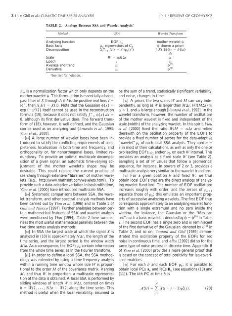
TABLE 2. Analogy Between SSA and Wavelet Analysis a
Method SSA Wavelet Transform
Analyzing function EOF k mother wavelet
Basic facts k eigenvectors of CX chosen a priori
M
Decomposition ¥ t1 X(t t) k(t) X(t)((t b)/a)
dt
Scale W Mt a
Epoch t b
Average and trend 1 (0)
Derivative 2 (1)
a See text for notation.
A is a normalization factor which only depends on the
mother wavelet . This formulation is essentially a bandpass
filter of X through I; ifIis the positive real line, I
, then XI(t) X(t). Note that the Gaussian ( x)
exp (x 2 / 2) itself cannot be used in the reconstruction
formula (19), because it does not satisfy ( x) dx
0, although its first derivative does. The forward transform
of (18), however, is well defined, and the Gaussian
can be used as an analyzing tool [Arneodo et al., 1993;
Yiou et al., 2000].
[88] A large number of wavelet bases have been introduced
to satisfy the conflicting requirements of completeness,
localization in both time and frequency, and
orthogonality or, for nonorthogonal bases, limited redundancy.
To provide an optimal multiscale decomposition
of a given signal, an automatic time-varying adjustment
of the mother wavelet’s shape may be
desirable. This could replace the current practice of
searching through extensive “libraries” of mother wavelets
(e.g., http://www.mathsoft.com/wavelets.html). To
provide such a data-adaptive variation in basis with time,
Yiou et al. [2000] have introduced multiscale SSA.
[89] Systematic comparisons between SSA, the wavelet
transform, and other spectral analysis methods have
been carried out by Yiou et al. [1996] and in Table 1 of
Ghil and Taricco [1997]. Further analogies between certain
mathematical features of SSA and wavelet analysis
were mentioned by Yiou [1994]. Table 2 here summarizes
the most useful mathematical parallels between the
two time series analysis methods.
[90] In SSA the largest scale at which the signal X is
analyzed in (10) is approximately Nt, the length of the
time series, and the largest period is the window width
Mt. As a consequence, the EOFs k contain information
from the whole time series, as in the Fourier transform.
[91] In order to define a local SSA, the SSA methodology
was extended by using a time-frequency analysis
within a running time window whose size W is proportional
to the order M of the covariance matrix. Varying
M, and thus W in proportion, a multiscale representation
of the data is obtained. A local SSA is performed by
sliding windows of length W Nt, centered on times
b W/2, , Nt W/ 2, along the time series. This
method is useful when the local variability, assumed to
be the sum of a trend, statistically significant variability,
and noise, changes in time.
[92] A priori, the two scales W and M can vary independently,
as long as W is larger than Mt, W/(Mt)
1, and is large enough [Vautard et al., 1992]. In the
wavelet transform, however, the number of oscillations
of the mother wavelet is fixed and independent of the
scale (width) of the analyzing wavelet. In this spirit, Yiou
et al. [2000] fixed the ratio W/M t and relied
therewith on the oscillation property of the EOFs to
provide a fixed number of zeroes for the data-adaptive
“wavelet” k of each local SSA analysis. They used
3 in most of their calculations, as well as only the one or
two leading EOFs, 1 and/or 2, on each W interval. This
provides an analysis at a fixed scale W (see Table 2).
Sampling a set of W values that follow a geometrical
sequence, for instance, in powers of 2 or 3, provides a
multiscale analysis very similar to the wavelet transform.
[93] For a given position b and fixed W, we thus
obtain local EOFs that are the direct analogs of analyzing
wavelet functions. The number of EOF oscillations
increases roughly with order, and the zeroes of k1
separate those of k; this emulates an important property
of successive analyzing wavelets. The first EOF thus
corresponds approximately to an analyzing wavelet function
with a single extremum and no zero inside the
window, for instance, the Gaussian or the “Mexican
hat”; such a basic wavelet is denoted by (0) in Table
2. The second EOF has a single zero and is reminiscent
of the first derivative of the Gaussian, denoted by (1) in
Table 2, and so on. Vautard and Ghil [1989] demonstrated
this oscillation property of the EOFs for red
noise in continuous time, and Allen [1992] did so for the
same type of noise process in discrete time. Appendix B
of Yiou et al. [2000] provides a more general proof that
is based on the concept of total positivity for lag-covariance
matrices.
[94] For each b and each EOF k, it is possible to
obtain local PCs A k and RCs R k (see equations (10) and
(11)). The kth PC at time b is
M
b b
Akt j1 Xt j 1k j, (20)