advanced spectral methods for climatic time series - Atmospheric ...

40, 1 / REVIEWS OF GEOPHYSICS Ghil et al.: CLIMATIC TIME SERIES ANALYSIS ● 3-23
[149] Mann and Lees [1996] provide a robust estimate
of the spectral background (equation (13)) by minimizing,
as a function of r, the misfit between an analytical
AR(1) red-noise spectrum and the adaptively weighted
multitaper spectrum convolved with a median smoother.
The median smoothing operation insures that the globally
estimated noise background is insensitive to “outliers.”
These outliers may be due to peaks associated
with significant signals or to spurious ones. The median
smoother guards against inflated estimates of noise variance
and noise autocorrelation; the latter arise in a
conventional Box-Jenkins approach due to the contamination
of noise parameters by contributions from the
signal, for example, from a significant trend or oscillatory
component of the series. A median smoothing width
of f min ( f N/4, 2pf R) is a good compromise between
describing the full variation of the background
spectrum over the Nyquist interval, on the one hand, and
insensitivity to narrow spectral features, on the other.
[150] Significance levels for harmonic or narrowband
spectral features relative to the estimated noise background
can be determined from the appropriate quantiles
of the chi-square distribution, by assuming that the
spectrum is distributed with 2K degrees of freedom
[Mann and Lees, 1996]. A reshaped spectrum is determined
in which the contributions from harmonic signals
are removed [Thomson, 1982], based on their passing a
significance threshold for the F test on the variance
ratio, as described above. In this way, noise background,
harmonic, and narrowband signals are isolated in two
steps. The harmonic peak detection procedure provides
information as to whether the signals are best approximated
as harmonic or narrowband, i.e., as phase-coherent
sinusoidal oscillations or as amplitude-and-phase–
modulated, and possibly intermittent, oscillations. In
either case, they must be found to be significant relative
to a specified noise hypothesis, such as that of red noise
(equation (13)) used above.
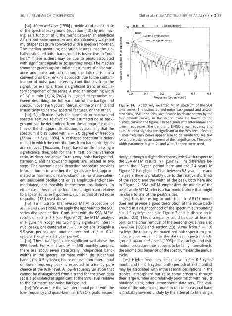
[151] To illustrate the revised MTM procedure of
Mann and Lees [1996], we apply the approach to the SOI
series discussed earlier. Consistent with the SSA-MEM
results of section 3.3 (see Figure 12), the MTM analysis
in Figure 14 recognizes two highly significant interannual
peaks, one centered at f 0.18 cycle/yr (roughly a
5.5-year period) and another centered at f 0.41
cycle/yr (roughly a 2.5-year period).
[152] These two signals are significant well above the
99% level: For p 2 and N 690 monthly samples,
there are about seven statistically independent bandwidths
in the spectral estimate within the subannual
band ( f 0.5 cycle/yr); hence not even one interannual
or lower-frequency peak is expected to arise by pure
chance at the 99% level. A low-frequency variation that
cannot be distinguished from a trend for the given data
set is also isolated as significant at the 99% level relative
to the estimated red-noise background.
[153] We associate the two interannual peaks with the
low-frequency and quasi-biennial ENSO signals, respec-
Figure 14. Adaptively weighted MTM spectrum of the SOI
time series. The estimated red-noise background and associated
90%, 95%, and 99% significance levels are shown by the
four smooth curves, in this order, from the lowest to the
highest curve in the figure. Three signals with interannual and
lower frequencies (the trend and ENSO’s low-frequency and
quasi-biennial signals) are significant at the 99% level. Several
higher-frequency peaks appear also to be significant; see text
for a more detailed assessment of their significance. The bandwidth
parameter is p 2, and K 3 tapers were used.
tively, although a slight discrepancy exists with respect to
the SSA-MEM results in Figure 12. The difference between
the 2.5-year period here and the 2.4 years in
Figure 12 is negligible. That between 5.5 years here and
4.8 years there is probably due to the relative shortness
of the record and the width of the peak, both here and
in Figure 12. SSA-MEM emphasizes the middle of the
peak, while MTM selects a harmonic feature that might
lie close to one of the peak’s sides.
[154] It is interesting to note that the AR(1) model
does not provide a good description of the noise background
in a neighborhood of the spectrum surrounding
f 1.0 cycle/yr (see also Figure 7 and its discussion in
section 2.3). This discrepancy could be due, at least in
part, to the prior removal of the seasonal cycle (see also
Thomson [1995] and section 2.3). Away from f 1.0
cycle/yr the robustly estimated red-noise spectrum provides
a good visual fit to the data set’s spectral background.
Mann and Lees’s [1996] noise background estimation
procedure thus appears to be fairly insensitive to
the anomalous behavior of the spectrum near the annual
cycle.
[155] Higher-frequency peaks between f 0.3 cycle/
month and f 0.5 cycle/month (periods of 2–3 months)
may be associated with intraseasonal oscillations in the
tropical atmosphere but raise some concerns through
their large number and relatively poor match with results
obtained using other atmospheric data sets. The estimate
of the noise background in this intraseasonal band
is probably lowered unduly by the attempt to fit a single